The Bohr Model of Hydrogenic Ions

The Bohr Model of Hydrogenic Ions 

Introduction 

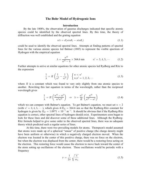
By the late 1800's, the observation of gaseous discharges indicated that specific atomic 

species could be identified by the observed spectral lines. By this time, the theory of 

diffraction was well established and the grating equation 

8- œ .Ð=38) < =38) 

3 Ñ 

(1.1) 

could be used to identify the observed spectral lines. Attempts at finding patterns of spectral 

lines for the various atomic species led Balmer (1885) to represent the visible spectrum of 

Hydrogen with the empirical equation 

w# 

8 

w 

- œ ‚ 364.6 nm 8 œ 3 ß %ß &ß â (1.2) 

8w# 

% 

Further attempts to arrive at similar equations for other atomic species led Rydberg and Ritz to 

the expression 

" " " 

w 

8 8 

œ V Œ 

- 8# 8w# 

œ w 

8, 

8 œ "ß #ß $ß â 

where V is a constant which was found to vary only slightly from one atomic species to 

another. Rewriting this last equation in terms of the wavelength, rather than the reciprocal 

wavelength gives 

(1.3) 

w# # # w# 

" 8 8 8 8 

œ V Œ Ê - œ 

(1.4) 

- 8# Œ 

8w# V 8w# 8# 

which we can compare with Balmer's equation. To get Balmer's equation, we must set 8 œ 2 

w 

(with 8 œ $ß %ß &ß â ), which gives 4/ VL 

œ 364.6 nm so that the Rydberg-Ritz constant for 

( " 

hydrogen is given by VL 

œ 1.0971 ‚ 10 m . It should be obvious that if the Rydberg-Ritz 

equation is correct, other spectral lines of hydrogen should exist. Experimenters soon began to 

look for these lines and did discover some of these additional lines. Although the Rydberg- 

Ritz formula helped to give some order to the observed spectral lines, there was no adequate 

theory which predicted such a regular series of lines. 

At this time, there were two prevailing models for atoms. Thompson's model assumed 

that atoms were made up of a spherical “smear” of positive charge (the charge density might 

have been uniform or otherwise) in which a negatively charged electron moved. When the 

electron was located in the center of this positive charge, there was no force on the electron, 

but when the electron was displaced from the center, there would be a restoring force acting on 

the electron. This restoring force would cause the electron to move back toward the center of 

the atom setting up oscillations of the electron. These oscillations would be periodic with a 

frequency 

, 

/ œ " 

# 1 7 

Ê 

/ 

(1.5)

The Bohr Atom 2 

where , is an equivalent “spring constant”, and 7 / is the mass of the electron. As the electron 

oscillated within the atom, the moving electron would radiate electromagnetic energy of the 

same frequency as the oscillating electron. In addition, the energy loss due to radiation would 

eventually bring the electron to rest within the atom, and the “damping” of the oscillations due 

to the radiation should show up as a broadening of the spectral lines. This model does, in fact, 

do a very favorable job in predicting line shapes. However, it does not adequately describe 

why a single atomic species should exhibit many different spectral lines. 

The so-called planetary model of the atom was based upon the experimental findings of 

Rutherford. Following Becquerel's discovery of natural radioactivity in 1896, Rutherford 

studied the emissions of these radioactive materials. He was able to classify two different 

types of radiation, α -radiation, and "-radiation. By doing charge-to-mass measurements on 

these particles emitted from a radioactive nucleus, he was able to determine that the α particle 

was simply a He nucleus. Since these α particles were emitted with a fixed energy, they 

proved an ideal tool to probe the atom in an attempt to understand the atomic structure. When 

Rutherford and his two graduate students, Geiger and Marsden, began to study the collisions of 

α particles with thin foils, they discovered that most of the α particles were not deflected, and 

that those that were deflected were deflected by relatively large amounts. (The Thompson 

model of the atom predicted only very small deflections of the incoming α particle.) To 

explain the very large backscattering of the α particles one has to assume that the mass of the 

"& 

atom is concentrated in a very small volume, the radius of which is of the order of 10 m. 

Based upon x-ray scattering experiments, where x-rays were scattered from atomic planes 

"! 

within crystals, the interatomic distance was believed to be of the order of 10 m. This 

meant that the positive charge and most of the mass of the atom was confined in a very small 

“nucleus” and that the rest of the atom was essentially empty (small light electrons would have 

to swarm about this nucleus to produce an atom). One of the fundamental problems of this 

model is the fact that moving charges should radiate energy. Electrons moving around the 

nucleus would, therefore, loose some of their energy and would eventually fall into the 

nucleus, collapsing the atom! 

The Bohr Atom 

In 1913, Bohr proposed a model of the hydrogen atom which is based upon the planetary 

model, and which incorporated some of the ideas that had been developed by Planck and 

Einstein in the explanation of blackbody radiation and the photoelectric effect. He first 

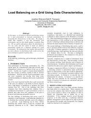
assumed that the electron orbits the nucleus (a single proton) in a simple circular path as 

shown below. 

e 

Ze 

r


The magnitude of the electrostatic force of attraction between the nucleus and the electron 

is given by 

J œ 5Ð^/Ñ/ 

< # (1.6) 

where 5 is the Coulomb constant (often expressed as 1/41% 9 ), < is the distance between the 

nucleus and the electron, / is the charge of the electron, and ^/ is the charge of the nucleus for 

a “hydrogenic” ion (any ion with only one electron orbiting the nucleus). This electrostatic 

# 

force is the centripetal force acting on the electron and must be equal to 7@ Î< , giving 

or 

5Ð^/Ñ/ 7@ 

œ 

< 

# 

< 

# 

7@ œ 5Ð^/Ñ/ 

< 

Thus far, we have not introduced anything which is non-classical in our model. Let's 

examine the result of assuming that the frequency of radiation is just the classical frequency of 

revolution. The velocity of the electron is related to the “frequency” of revolution of the 

electron by the equation @ œ = < œ # 1 / < , and thus to the frequency of radiation emitted from 

the atom. From our last equation, we have 

or 

# 

(1.7) 

(1.8) 

# # 

7@ œ 7 # 1/ < œ 5Ð^/Ñ/ 

(1.9) 

< 

/ œ " Ê 

5^/ 

# 1 7< 

$ 

# 

(1.10) 

We want to use this last equation to calculate a numerical value for the frequency / (and thus 

the wavelength). To do this, we use some “tricks” to get useful combinations of constants and 

we let ^ œ 1 for hydrogen and < " A. ° 

" ( 5/ 

#)-# " Í (14.4 eV-A) ° -# " (14.4 eV) -# 

/ œ œ œ 

# 1 

Ë 

( 7- 

#) 

< 

$ 

# 1 Ì (511 keV)(1 A) ° $ # 1 Ë 

(5.11 ‚ 10 

& 

eV)(1 A) ° # 

from which we obtain 

or, since -/ œ -, 

"& " 

/ œ 2.534 ‚ "! sec 

- œ 1183.6 A. °


This value agrees very well with the observed wavelength of the Lyman- α line, 1215.7 A, ° 

indicating that the Bohr model may have some validity. But there still remains a thorny 

problem. If the electron radiates energy as it moves in its orbit, the electron must loose energy, 

and therefore spiral inward toward the nucleus, eventually collapsing. Thus, this picture is not 

complete. 

In an attempt to circumvent this classical collapse, Bohr looked to the findings of 

Einstein and Planck. Since the energy of electromagnetic waves seem to come in packets of 

size 2/ , Bohr postulated that the energy emitted from an atom must be emitted in dicrete 

chunks of energy equal to 2/ . Thus, Bohr postulated that an electron could exist is some 

orbiting state within the atom without radiating, but if the electron were to change from one 

stable state to another, the energy change in the atom must be equal to the energy emitted by 

the photon, or 

I I œ 2 

0 3 / (1.11) 

To continue this line of reasoning, we must look for an expression for the total energy of 

the atom. This is accomplished by combining the kinetic energy of the electron and the 

electrostatic potential energy of the atom. The kinetic energy of the electron is related to the 

electrostatic force by Equation 1.6, from which we can write 

The electrostatic potential energy of the electron is given by 

which gives 

" 5Ð^/Ñ/ 

7@ # œ 

(1.12) 

# # < 

Y Ð


The total energy of the electron in it's orbit around the nucleus is the sum of the kinetic 

and potential energies 

" 5Ð^/Ñ/ 5^/ / " 5^/ / 

I œ I538 I:9> 

œ œ 

# < < # < 

Bohr's hypothesis, then, leads us to the equation 

which can be written 

" 5 ^/ / " 5 ^/ / 

I0 I3 

œ 2 / œ ” 

 

# < • ” 

# < 

• 

0 3 

(1.15) 

(1.16) 

2- 5Ð^/Ñ/ " " 

I0 I3 œ 2/ 

œ œ ” • 

- # <


and we obtain an expression for the radius given by 

# 

< œ P 

5^7/ 

Bohr, using arguments similar to Planck's, postulated that the angular momentum was 

quantized and had the form 

# 

P œ 8h (1.20) 

where h œ 2Î# 1, with 2 being Planck's constant. The radius of a Bohr orbital, then, is given 

by 

# # # 

8 h 8 

< œ œ + 

^57/ 

# o (1.21) 

^ 

where + o is some constant. The relationship for the energy levels of an electron within a 

hydrogenic atom is now given by 

# 

o 

# # 

# # 

5 ^/ 7/ I 

I8 

œ œ 

# 8h 

8 

(1.22) 

where Io 

is the ground state energy (the state where 8 œ "). This is just the energy that must 

be added to the electron in the ground state to ionize the atom, and is, therefore, the ionization 

potential energy. For hydrogen, the ionization potential was known to be approximately 13.6 

eV. The ground state energy for Bohr's model of the hydrogen atom (where ^ œ ") is given 

by 

# 

# % # # $ 

75 / 7- 5/ c&"" ‚ "! eVdc"Þ%% MeV † fmd 

Io 

œ œ œ œ "$Þ'" 

#h# 

# # 

eV (1.23) 

# h- # c"*(Þ$ MeV † fmd 

in excellent agreement with the ionization potential for hydrogen. In addition, the radius of the 

first Bohr orbital, the orbit with the lowest (or ground state) energy level is given by 

+ œ h # 

o 

(1.24) 

75/ 

# 

Evaluating this to determine the size of the first Bohr orbit we obtain 

# # 

h- c"*(Þ$ MeV † fmd 

‰ 

+ o œ œ œ !Þ&#* A (1.25) 

7-# 5/ 

# 

c!Þ&"" MeV dc"Þ%%! MeV † fmd 

in excellent agreement with the known size of atoms. 

At this point, we have found the predicted energy levels for Bohr's hypothetical 

stationary states, and the corresponding electron orbital radii for these states. Both the 

energies and the radii are quantized as expected. In addition, we find that the angular 

momentum of the electron is also quantized. The quantized nature of the energy levels is just 

what is needed to give the discrete spectrum observed for hydrogen and other atoms. The 

#


predicted wavelengths for these lines can be determined by applying Bohr's equation 

2- 

2/ 

œ œ I I 

- 

0 3 

(1.26) 

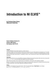
An energy diagram of the hydrogen atom is shown below, where the ground state 

energy has been assigned zero energy. The actual total energy of an electron which is bound to 

the hydrogen atom is negative and the allowed energies are given by 

I œ I o 

8 

8# 

(1.27) 

which gives the ground state energy equal to "$Þ' eV, the next higher energy level as $Þ% 

eV, and the energy of a free electron as zero. In the diagram below, we have simply shifted the 

energy levels upward by an amount equal to the ground state energy. This allows us to plot the 

energy of each successive level relative to the ground state. The second energy level is 

indicated as 10.2 eV above the ground state. Also indicated on this energy level diagram is the 

wavelength of a photon emitted when an electron changes from one energy level to another. 

The lines shown on this diagram are the Lyman series which occur in the ultraviolet region of 

the spectrum. The linear spacing between the verticle lines is proportional to the actual 

wavelengths of the emitted line. You can see that the wavelengths of the emitted photons get 

closer and closer at the low wavelength limit and eventually “pile up” at the low wavelength 

limit, which is given by 

or 

2- 

2/ 

œ œ "$Þ' eV (1.28) 

- 

- œ *""Þ) ‰ A (1.29) 

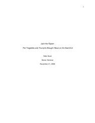
The next diagram shows some of the possible transitions that can arise when an electron 

moves from one energy level to another (not just the ground state energy level). It turns out 

that only certain types of transitions are allowed! This gives rise to so-called selection rules 

for electonic transitions, and further restricts the possible wavelengths that can be observed 

from a given atomic species. 

Note: One can show that the energy levels of an electron withing a hydrogenic atom are 

related to the square of the angular momentum using the following “trick”. If we square the 

first term of the equation 

and divide by 

# 

7@ Î# , we have 

# 

" 5^/ / 7@ 

I œ œ œ IoÎ8 

# < # 

# 

# # # # # # # 

# 5 ^/ / 7@ 5 ^/ / 

I œ I ƒ I œ ƒ œ 

%


which can be written 

I œ 

# # # # # # 

5 ^/ 7/ 5 ^/ 7/ 

# 

œ 

# 7@< #P# 

 

(1.31) 

where P is the angular momentum. This demonstrates that the total energy of the electron is 

inversely proportional to the square of the angular momentum. This fact may have led Bohr to 

postulate that the angular momentum of the electron within the atom was quantized, giving 

7@< œ P œ 8-98=>+8> 

 

14 

Hydrogen Atom Energy Level Diagram 

12 

10 

Energy (eV) 

8 

6 

972.53 

949.74 

4 

1025.72 

2 

1215.66 

0 

Wavelengths


n=4 

n=3 

Paschen 

n=2 

Balmer 

n=1 

Lyman


Summary of Equations for Bohr's Model 

of Hydrogenic Atoms 

The energy of the bound electron is given by: 

# Io 

7- 5/ 

 

I8 

œ ^ where I œ œ "$Þ'" 

8 

# 

o 

# 

eV 

# h- 

The radii of the electron orbitals are given by: 

# # # 

# + o 

h- 

‰ 

< 8 œ 8 where + o œ œ !Þ&#* A 

^ 7-# 5/ 

# 

The energy carried away by a photon as an electron drops from a higher energy state to a lower 

energy state is given by: 

2- # # " " 

2/ 

œ œ I0 I3 

œ ^ I 

- 

o 8 8 Ÿ 

# 

# # 

0 3 

From this last equation we can determine the possible wavelengths which can be emitted from 

the atom: 

# # 

" " " ^ I 

œ VD 

V œ 

- D 

8# 8# Ÿ where o 

3 2- 

0


Corrections to the Bohr Model 

In deriving the Bohr model of a hydrogenic atom (or ion), we assumed that the electron 

orbited a fixed nucleus. In order to correct for that assumption, we need to look at the situation 

where both the nucleus and the electron can move (i.e., both particles have kinetic energy). 

Let us assume that the distance between the nucleus and the electron is fixed at some distance 


This means we can express the kinetic energy equation as 

# 

# # # # # 

OI œ " ˆ QV 7V ‰ œ " QV 7 Q 

" # = V 

# # " Œ " 

7 = 

" Q 

œ ŒQ V 

# 7 

# 

" # = 

# 

(1.36) 

which can also be written in terms of the distance between the proton and electron as 

or 

# # 

" Q " 7Q Q 7 

OI œ ŒQ V" # = # œ Œ Œ V 

# = # (1.37) 

# 7 # 7 Q 7 

# 

" 7 Q 7 # # " 7Q # # " # # 

OI œ Œ Œ QV = œ Œ V = œ . V = (1.38) 

# 7 Q 7 # Q 7 # 

where . is the reduced mass of the system. This is the same expression for the kinetic energy 

that would arise from a single particle of mass . moving is a circle of radius V with a velocity 

given by @ œ = V. Thus, we can correct for the motion of the nucleus simply by using the 

reduced mass . in place of the mass of the electron. 

This would imply (because our results for the hydrogen atom seem to work so well) 

that the reduced mass must be approximately equal to the mass of the electron. Let's express 

the reduced mass in terms of the ratio of the mass of the electron to the mass of the nucleus as 

seen in the next equation. 

7Q 7 7/ 

. œ œ œ 

Q 7 " 7- # 

" !Þ!!!&% 

Q- 

# 

# 

(1.39) 

If the mass of the electron is very small relative to the mass of the nucleus, then the term 

7ÎQ in the denominator can be eccentially ignored. In fact, the proton rest mass energy is 

approximately 2000 times larger than the rest mass energy of the electron, so that the reduced 

mass is very nearly equal to the mass of the electron (only about 0.05% smaller). This does 

give a slightly different value for the energies, wavelengths, and radii of the Hydrogen atom 

than what we obtained earlier. The corrected ground state energyß 

for example, is given by 

I œ "$Þ'! /Z 

! -9

The Bohr Model of Hydrogenic Ions

Create successful ePaper yourself

Delete template?

Save as template?