AN OPTIMAL DISTRIBUTED ROUTING ALGORITHM USING DUAL ...

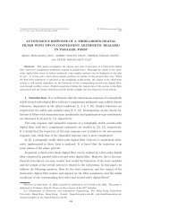
288 PUNYASLOK PURKAYASTHA AND JOHN S. BARAS
Table 1
Optimal flows and ‘potentials’ (C 13 = 10, C 21 = 4, C 32 = 4, C 34 = 14, C 24 = 4)
Optimal link flows Optimal node potentials
F13 ∗ = 6.89 p∗ 1 = 3.19
F21 ∗ = 0.89 p∗ 2 = 3.48
F24 ∗ = 3.11 p ∗ 3 = 0.97
F34 ∗ = 6.89 p ∗ 4 = 0.00
F32 ∗ = 0.00
The network that we consider is shown in Figure 1. There are incoming traffic
flows at nodes 1 and 2, and the destination node is 4. The incoming traffic rates
at nodes 1 and 2 are r 1 = 6 and r 2 = 4. C ij denotes the capacities of the links
(i, j). In what follows, we assume that β = 1 and that the delay functions are of
the form D ij (F ij ) =
1
C ij−F ij
. (This is the commonly made M/M/1 approximation,
also referred to as “Kleinrock’s independence assumption” [3].) This delay function
satisfies our assumptions (A1) and (A2). We now set up the gradient algorithm.
For this case, the relations (18) and (19) reduce to
F ij (p n i − p n j ) = 0, if p n i − p n j ≤ 0,
F ij (p n i − pn j ) = (pn i − pn j )C ij
1 + p n i − , if p n
pn i − pn j > 0.
j
We set up the gradient algorithm with a small constant step-size, i.e., α n = α, for
some small positive α, and start with an arbitrary initial dual vector p 0 . Each dual
vector component is updated using the equation
(
= p n i + α ∑
F ji (p n j − pn i ) −
p n+1
i
j:(j,i)∈L
∑
j:(i,j)∈L
F ij (p n i − pn j ) + r i
where F ij (p n i − pn j ) and F ji(p n j − pn i ) are computed using the above equations.
The capacities of the links are C 13 = 10, C 21 = 4, C 32 = 4, C 34 = 14, C 24 = 4,
and α is set equal to 0.05. The optimal flows and potentials with this setting are
tabulated in Table 1.
Keeping the capacities of the other links fixed, we can increase the capacity C 24
until the entire flow that arrives at node 2 goes through the link (2, 4) and no fraction
traverses (2, 1). This happens when C 24 is increased to 8. The optimal flows and
potentials that result are tabulated in Table 2.
If we now further increase the capacity C 24 , because the flow coming in at node 3
now sees an additional available path that goes through node 2 to node 4 and which
has high capacity, a fraction of the flow arriving at 3 goes through this path. The
optimal flows and potentials when C 24 is set at 16 are tabulated in Table 3.
The optimal flow allocations on links thus vary as the capacities vary relative to
each other. In fact the routing algorithm can be seen as accomplishing a form of re-
)
,