AN OPTIMAL DISTRIBUTED ROUTING ALGORITHM USING DUAL ...

COMMUNICATIONS IN INFORMATION AND SYSTEMS 

c○ 2008 International Press 

Vol. 8, No. 3, pp. 277-302, 2008 005 

AN OPTIMAL DISTRIBUTED ROUTING ALGORITHM USING 

DUAL DECOMPOSITION TECHNIQUES ∗ 

PUNYASLOK PURKAYASTHA † AND JOHN S. BARAS † 

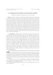
Abstract. We consider the routing problem in wireline, packet-switched communication networks. 

We cast our optimal routing problem in a multicommodity network flow optimization framework. 

Our cost function is related to the congestion in the network, and is a function of the flows on 

the links of the network. The optimization is over the set of flows in the links corresponding to the 

various destinations of the incoming traffic. We separately address the single commodity and the 

multicommodity versions of the routing problem. We consider the dual problems, and using dual 

decomposition techniques, we provide primal-dual algorithms that converge to the optimal solutions 

of the problems. Our algorithms, which are subgradient algorithms to solve the corresponding dual 

problems, can be implemented in a distributed manner by the nodes of the network. For online, adaptive 

implementations of our algorithms, the nodes in the network need to utilize ‘locally available 

information’ like estimates of queue lengths on outgoing links. We show convergence to the optimal 

routing solutions for synchronous versions of the algorithms, with perfect (noiseless) estimates of 

the queueing delays. Every node of the network controls the flows on the outgoing links using the 

distributed algorithms. For both the single commodity and multicommodity cases, we show that our 

algorithm converges to a loop-free optimal solution. Our optimal solutions also have the attractive 

property of being multipath routing solutions. 

1. Introduction. We consider in this paper the routing problem in wireline, 

packet-switched communication networks. Such a network can be represented by a 

directed graph G = (N, L), where N denotes the set of nodes and L the set of directed 

links of the network. For such a network we are given a set of origin-destination (OD) 

node pairs, with a certain incoming traffic rate (in packets per sec) associated with 

each OD pair. The arriving packets at the origin node have to be transported by 

the network to the corresponding destination node of the OD pair. The routing 

objective is to establish a packet traffic flow pattern so that packets are directed to 

their respective destinations while, at the same time, minimizing congestion in the 

network. A typical framework for accomplishing the same involves setting up an 

optimization problem, with the cost being related to the network-wide congestion 

and the constraints being the natural flow conservation relations in the network. For 

large-scale networks which are of interest to us, it is desired that the routing solution 

be implementable in a decentralized manner by the nodes of the network. 

∗ Dedicated to Roger Brockett on the occasion of his 70th birthday. 

† The authors are with the Institute for Systems Research and the Department of Electrical and 

Computer Engineering, University of Maryland College Park, USA. Research supported by the U.S. 

Army Research Laboratory under the CTA C & N Consortium Coop. Agreement DAAD19-01-2- 

0011, the National Aeronautics and Space Administration under Coop. Agreement NCC8235, and 

by the U.S. Army Research Office under MURI01 Grant No. DAAD19-01-1-0465 and under Grant 

No. DAAD19-02-1-0319. 

277

278 PUNYASLOK PURKAYASTHA AND JOHN S. BARAS 

An early important work on optimal routing for packet-switched communication 

networks was Gallager [20]. The cost considered was the sum of all the average link 

delays in the network, and a distributed algorithm was proposed to solve the problem. 

The algorithm preserved loop-freedom after each iteration, and converged to an optimal 

routing solution. Bertsekas, Gafni, and Gallager [4] proposed a means to improve 

the speed of convergence by using additional information of the second derivatives of 

link delays. Both the algorithms mentioned above require that related routing information 

like marginal delays be passed throughout the network before embarking on 

the next iteration. Another cost function that has been considered in the literature is a 

sum of the integrals of queueing delays; see Kelly [22] and Borkar and Kumar [8]. The 

solution to this problem can be characterized by the so-called Wardrop equilibrium 

[31] - between a source-destination pair, the delays along routes being actively used 

are all equal, and smaller than the delays of the inactive routes. Another formulation 

of the optimal routing problem, called the path flow formulation (see Bertsekas [1] and 

Bertsekas and Gallager [3]), has been in vogue. Tsitsiklis and Bertsekas [29] considered 

this formulation, and used a gradient projection algorithm to solve the optimal 

routing problem in a virtual circuit network setting. They also proved convergence 

of a distributed, asynchronous implementation of the algorithm. This formulation 

was considered by Elwalid, Jin, Low, and Widjaja [18] to accomplish routing in IP 

datagram networks using the Multi-Protocol Label Switching (MPLS) architecture. 

The routing functionality is shifted to the edges of the network (a feature of the path 

flow formulation; this is also known as ‘source routing’), and requires measurements of 

marginal delays on all paths linking a source and a destination. Because the number of 

such paths could scale exponentially as the network size grows, it is not clear that the 

solution would scale computationally. Multipath routing and flow control based on 

utility maximization have also been considered, notably in Kar, Sarkar, and Tassiulas 

[21] and in Wang, Palaniswami, and Low [30]. Kar, Sarkar and Tassiulas propose an 

algorithm which uses congestion indicators to effect control of flow rates on individual 

links, but do not explicitly consider congestion indicators based on queueing delays 

as we do (their congestion indicators are based on flows on links). Their algorithm 

avoids the scalability issue mentioned above. On the other hand, Wang, Palaniswami, 

and Low consider a path flow formulation of the multipath routing and flow control 

problem, which as we have mentioned above has scalability problems. However, they 

do consider the effect of queueing delays, extracting related information by measuring 

the round trip times. Recently, dual decomposition techniques have been used by 

Eryilmaz and Srikant [19], Lin and Shroff [24], Neely, Modiano, and Rohrs [25], and 

Chen, Low, Chiang, and Doyle [15], to design distributed primal-dual algorithms for 

optimal routing and scheduling in wireless networks. Such techniques consider the 

dual to the primal optimization problem and exploit separable structures in the costs 

and/or constraints to come up with a decomposition which automatically points the

AN OPTIMAL DISTRIBUTED ROUTING ALGORITHM 279 

way towards distributed implementations. The seminal work of Kelly, Maulloo, and 

Tan [23] showed how congestion control can be viewed in this way. The approach 

(called Network Utility Maximization (NUM)) has gained currency and has been 

applied to a variety of problems in wireline and wireless communication networks, 

cutting across all layers of the protocol stack (see [16]). 

We cast our optimal routing problem in a multicommodity network flow optimization 

framework. Our cost function is related to the congestion in the network, 

and is a function of the flows on the links of the network. The optimization is over 

the set of flows in the links corresponding to the various destinations of the incoming 

traffic. We separately address the single commodity and the multicommodity versions 

of the routing problem. Our approach is to consider the dual optimization problems, 

and using dual decomposition techniques we provide primal-dual algorithms that converge 

to the optimal solutions of the problems. Our algorithms, which are subgradient 

algorithms to solve the corresponding dual problems, can be implemented in a distributed 

manner by the nodes of the network. For online, adaptive implementations 

of our algorithms, the nodes in the network need to utilize ‘locally available information’ 

like estimates of queue lengths on outgoing links. We show convergence to 

the optimal routing solutions for synchronous versions of the algorithms, with perfect 

(noiseless) estimates of the queueing delays (these essentially are the convergence 

results of the corresponding subgradient algorithms). Our optimal routing solution 

is not an end-to-end solution (our formulation is not a path-based formulation) like 

many of the above-cited works [29], [18], [30]. Consequently, our algorithms would 

avoid the scalability issues related to such an approach. Every node of the network 

controls the total as well as the commodity flows on the outgoing links using the 

distributed algorithms. Our optimal solutions also have the attractive property of being 

multipath routing solutions. Furthermore, by using a parameter (β) we can tune 

the optimal flow pattern in the network, so that more flow can be directed towards 

the links with higher capacities by increasing the parameter (we observe this in our 

numerical computations). 

The Lagrange multipliers (dual variables) can be interpreted as potentials on the 

nodes for the single commodity case, and as potential differences across the links for 

the multicommodity case.. Then, with every link of the network there is associated 

a characteristic curve (see Bertsekas [1] and Rockafellar [27]), which describes the 

relationship between the potential difference across the link and the link flow, the 

potential difference being thought of as ‘driving the flow through the link’. Using the 

relationships between the potential differences and the flows, we then provide simple 

proofs showing that our algorithm converges to a loop-free optimal solution, which is 

a desirable property. Our techniques are related to those employed in the literature 

on NUM methods. 

The methods, results and approach presented here make substantial contact with,


and indeed are inspired from, several ideas and results of Roger Brockett through the 

years. Indeed our costs are expressed as path integrals and our methods lead to 

gradient and subgradient optimization interpretation in a very concrete way. These 

ideas are related to the work of Brockett in [9, 13, 10]. Brockett often developed 

“electrical network” intuition for several diverse and seemingly unrelated problems – 

see for instance [13, 10, 14, 6, 11]. Our approach and solutions have very much such 

an “electrical network” intuition, see in particular the comments at the end of the first 

part of section 3 and the monographs of Dennis [17] and Rockafellar [27]. Network 

flow optimization is indeed a generalization of the assignment problem (see [1]). In 

this context our methods and approach result in gradient and subgradient algorithms 

(even distributed ones) to solve these network flow optimization problems. In this 

context our results are related to the work of Brocket and his research collaborators 

in [14, 6, 11]. As we state at the end of the first part of section 3 our methods amount 

to solving flow optimization problems via analog computation, an idea that Brockett 

developed even for discrete optimization problems [7]. The fact that the form of 

our costs was inspired by our earlier work on the convergence of the so called “Ant 

Routing Algorithm” [26], indicates the close interrelationships between the routing 

costs and the stability analysis of routing algorithms, in a spirit related to the early 

work of Brockett in [9]. Finally, recently Brockett has turned his attention to queuing 

networks – see [12] and more recent work. Indeed at a recent workshop he suggested 

to one of us (Baras) that our work on trust in communication networks and on the 

related problem area of collaboration among nodes in networks, could be given an 

“electrical network” interpretation and thus be treated via optimization methods and 

gradient-subgradient algorithms – a suggestion we are pursuing. 

Our paper is organized as follows. In the next section, we discuss the formulation 

of our optimal routing problem in detail. In Section 3 we investigate the special case of 

the single commodity problem, and in Section 4 we consider the general problem with 

multiple commodities (corresponding to different destinations of the incoming traffic). 

For both cases a few examples that illustrate the computations are also provided. 

2. General Formulation of the Routing Problem. We now describe in brief 

our formulation. Let r (k) 

i ≥ 0 denote the rate of input traffic entering the network 

at node i and destined for node k 1 . The flow on link (i, j) corresponding to packets 

bound for destination k is denoted by f (k) 

ij . The total flow on link (i, j) is denoted 

by F ij and is given by F ij = ∑ k∈N f(k) ij . All packet flows having the same node as 

destination are said to belong to one commodity, irrespective of where they originate. 

Let C ij denote the total capacity of link (i, j). At node i, for every outgoing link (i, j), 

there is an associated queue which is assumed to be of infinite size. Let D ij (F ij ) denote 

1 The arrival process is usually modeled as a stationary stochastic process, and r (k) 

i 

to the time averaged rate of the process. 

then refers


the average packet delay in the queue when the total traffic flow through (i, j) is F ij , 

with F ij satisfying the constraint 0 ≤ F ij < C ij . (Quantities F ij , r (k) 

i , f (k) 

ij and C ij 

are all expressed in the same units of packets/sec.) 

Let f denote the (column) vector of commodity link flows f (k) 

ij , (i, j) ∈ L, k ∈ N, 

in the network. We consider the following optimal routing problem: 

subject to 

(1) 

(2) 

(3) 

Problem (A) : Minimize the (separable) cost function 

G(f) = ∑ 

G ij (F ij ) = ∑ ∫ Fij 

u[D ij (u)] β du, 

∑ 

(i,j)∈L 

j:(i,j)∈L 

f (k) 

ij 

(i,j)∈L 

= r (k) 

i + ∑ 

j:(j,i)∈L 

0 

f (k) 

ji , ∀i, k ≠ i, 

f (k) 

ij ≥ 0, ∀(i, j) ∈ L, k ≠ i, 

f (i) 

ij = 0, ∀(i, j) ∈ L, 

F ij = ∑ k∈N 

f (k) 

ij , ∀(i, j) ∈ L, 

(4) 

with 0 ≤ F ij < C ij , ∀(i, j) ∈ L. 

In an earlier work on convergence of Ant-Based Routing Algorithms [26], we 

showed, for a simple network involving N parallel links between a source-destination 

pair of nodes, that the equilibrium routing flows were such that they solved an optimization 

problem with a similar cost function and with similar capacity constraints as 

above. The scheme also yielded a multipath routing solution. It was natural to look 

for a generalization for the network case that has similar attractive properties. We 

shall see, using dual decomposition techniques, that the solution to our (optimization) 

Problem (A) is also a multipath routing solution, which can be implemented 

in a distributed manner by the nodes in the network. Our cost function is related 

to the network-wide congestion as measured by the link delays, and is small if the 

link delays are small. (Other cost functions have been used in the literature: in Gallager 

[20] and Bertsekas, Gallager and Gafni [4] it is of the form (in our notation) 

D(f) = ∑ (i,j)∈L D ij(F ij ); and in the Wardrop routing formulation (see Kelly [22]) it 

is of the form W(f) = ∑ ∫ Fij 

(i,j)∈L 0 

D ij (u)du.) The parameter β in our cost can be 

used to change the overall optimal flow pattern in the network. Roughly speaking, a 

low value of β results in the flows being more ‘uniformly distributed’ on the paths, 

whereas a high value of β tends to make the flows more concentrated on links lying 

on higher capacity paths. 

Constraints (1) above are the per-commodity flow balance equations at the network 

nodes (flow out of the node = flow into the node), and constraints (3) express 

the fact that once a packet reaches its intended destination it is not routed back into 

the network. The optimization is over the set of link flow vectors f.


3. The Single Commodity Problem: Formulation and Analysis. We consider 

in this section the single commodity problem, which involves routing of flows 

to a common destination node, which we label as d. We restate the problem for this 

special case in the following manner: 

Problem (B) : Minimize G(F) = ∑ 

subject to 

(i,j)∈L 

G ij (F ij ) = ∑ 

(i,j)∈L 

∫ Fij 

0 

u[D ij (u)] β du, 

(5) 

(6) 

∑ 

F ij = r i + 

∑ 

F ji , ∀i ∈ N, 

j:(i,j)∈L 

j:(j,i)∈L 

F dj = 0, for (d, j) ∈ L, 

with 0 ≤ F ij < C ij , ∀(i, j) ∈ L. 

r i is the incoming rate for traffic arriving at node i, and destined for d. The optimization 

is over the set of link flow vectors F, whose components are the individual 

link flows F ij , (i, j) ∈ L. As usual, equations (5) give the flow balance equations at 

every node and equations (6) refer to the fact that once a packet reaches d, it is not 

re-routed back into the network. 

We use a dual decomposition technique of Bertsekas [1] to develop a distributed 

primal-dual algorithm that solves the above-stated optimal routing problem. We carry 

out our analysis under the following fairly natural assumptions. These assumptions 

are also used, almost verbatim, for the multicommodity version of the problem in 

Section 4. 

Assumptions: 

(A1) D ij (u) is a nondecreasing, continuously differentiable, positive real-valued 

function of u, defined over the interval [0, C ij ). 

(A2) lim u↑Cij D ij (u) = +∞. 

(A3) There exists at least one feasible solution of the primal Problem (B). 

Assumption (A1) is a reasonable one, because when the flow u through a link 

increases, the average queueing delay (which is a function of the flow u) increases too. 

Assumption (A2) is satisfied for most queueing delay models of interest. Assumption 

(A3) implies that there exists a link flow pattern in the network such that the incoming 

traffic can be accommodated without the flow exceeding the capacity in any link. 

We start the analysis by attaching prices (Lagrange multipliers) p i ∈ R, to the 

flow balance equations (5) and form the Lagrangian function L(F,p) 

L(F,p) = ∑ 

G ij (F ij ) + ∑ ( ∑ 

p i 

(i,j)∈L i∈N 

j:(j,i)∈L 

F ji + r i − 

∑ 

F ij 

), 

j:(i,j)∈L


a function of the (column) price vector p and the link flow vector F. We can rearrange 

the Lagrangian to obtain the following convenient form 

(7) L(F,p) = ∑ 

) 

(G ij (F ij ) − (p i − p j )F ij + ∑ p i r i . 

i∈N 

(i,j)∈L 

Using the Lagrangian, the dual function Q(p) can be found by 

Q(p) = inf L(F,p), 

where the infimum is taken over all vectors F, such that the components F ij satisfy 

0 ≤ F ij < C ij . 

From the form (7) for the Lagrangian function, we can immediately see that 

Q(p) = ∑ 

) 

inf 

(G ij (F ij ) − (p i − p j )F ij + ∑ p i r i , 

{F ij:0≤F ij


Minimize G ij (F ij ) − (p i − p j )F ij = ∫ F ij 

0 

u[D ij (u)] β du − (p i − p j )F ij 

subject to 0 ≤ F ij < C ij . 

The second derivative of G ij is G ′′ 

ij (F ij) = [D ij (F ij )] β + βF ij [D ij (F ij )] β−1 D ′ ij (F ij). 

Under our Assumption (A1), G ij (F ij ) is twice continuously differentiable and strictly 

convex on the interval [0, C ij ), so that the minimization problems above are all convex 

optimization problems on convex sets. We can show that for any price vector p (in 

particular, for an optimal dual vector p ∗ ), there exists a unique F ij ∈ [0, C ij ) (for 

every (i, j)) which attains the minimum in the above optimization problem (Lemma 

3, Appendix). 

Conditions equivalent to (9) that an optimal primal-dual pair (F ∗ ,p ∗ ) must satisfy 

are given by (for each (i, j) ∈ L) 

(10) 

F ∗ 

ij[D ij (F ∗ 

ij)] β ≥ p ∗ i − p ∗ j, if F ∗ 

ij = 0, 

F ∗ 

ij [D ij(Fij ∗ )]β = p ∗ i − p∗ j , if F ij ∗ > 0. 

(11) 

We also make the following observation. Suppose p ∗ i − p∗ j ≤ 0; then because for 

any F ij > 0, G ij (F ij ) − (p ∗ i − p∗ j )F ij = ∫ F ij 

u[D 

0 ij (u)] β du − (p ∗ i − p∗ j )F ij > G ij (0) − 

(p ∗ i − p∗ ∗ 

j ).0 = 0, Fij = 0 must then be the unique global minimum. Now, consider the 

contrapositive of (10) : if p ∗ i − p∗ j > 0 then F ij ∗ > 0. Thus, if p∗ i − p∗ j > 0 then F ij ∗ is 

positive, and is given by the solution to the nonlinear equation 

F ∗ 

ij [D ij(F ∗ 

ij )]β = p ∗ i − p∗ j . 

Because D ij is a nondecreasing and continuously differentiable function, the above 

equation has a unique solution for F ∗ 

ij . 

To summarize, an optimal primal-dual pair (F ∗ ,p ∗ ) is such that the following 

relationships are satisfied for each link (i, j), 

(12) 

(13) 

F ∗ 

ij = 0, if p ∗ i − p ∗ j ≤ 0, 

F ∗ 

ij [D ij(F ∗ 

ij )]β = p ∗ i − p∗ j , if p∗ i − p∗ j > 0, 

and in this case Fij ∗ > 0. In analogy with electrical networks, the relations above 

can be interpreted as providing the ‘terminal characteristics’ of the ‘branch’ (i, j). 

The Lagrange multipliers p ∗ i can be thought of as ‘potentials’ on the nodes, and the 

flows Fij ∗ as ‘currents’ on the links. The branch can be thought of as consisting of 

an ideal diode in series with a nonlinear current-dependent resistance. The difference 

of the ‘potentials’ or ‘voltage’ p ∗ i − p∗ ∗ 

j , when positive, drives the ‘current’ or flow Fij 

through a nonlinear flow-dependent resistance according to the law defined by (13). 

This analogy with electrical circuit theory helps in developing intuition. It was known 

(for the case of a quadratic cost function) to Maxwell, and was exploited by Dennis 

[17], who suggested that flow optimization problems with separable convex costs can 

be solved by setting up an electrical network with arcs having terminal characteristics


that can be derived in the same way as for our case. Once the network reaches 

equilibrium (starting from some initial condition), the currents and potentials can be 

simply ‘read off’ and are the optimal solutions to the primal and dual optimization 

problems, respectively. This amounts to solving the flow optimization problem using 

analog computation. 

3.1. Distributed Solution of the Dual Optimization Problem. We now 

focus on solving the dual problem using a distributed primal-dual algorithm. We first 

make a quick remark on the differentiability properties of the dual function Q(p). It 

can be verified that, for each (i, j) and (j, i), the partial derivatives ∂Qij(pi−pj) and 

∂Q ji(p j −p i) 

∂p i 

exist for all p i ∈ R. Then, at any point p, the partial derivatives ∂Q(p) 

∂p i 

all exist and can be easily seen to be given by 

(14) 

∂Q(p) 

∂p i 

= ∑ 

j:(i,j)∈L 

∂Q ij (p i − p j ) 

∂p i 

+ ∑ 

j:(j,i)∈L 

∂p i 

∂Q ji (p j − p i ) 

∂p i 

+ r i , i ∈ N. 

The gradient vector ∇Q(p) can thus be evaluated at each point p. 

The dual optimization problem can now be solved by the following simple gradient 

algorithm starting from an arbitrary initial price vector p 0 

(15) p n+1 = p n + α n ∇Q(p n ), n ≥ 0, 

where {α n } is a suitably chosen step-size sequence that ensures convergence of the 

gradient algorithm to an optimal dual vector p ∗ . We now try to simplify the expression 

(14), and get it into a form that is suitable for computational purposes. 

We had shown earlier that the minimum in the equation 

) 

Q ij (p i − p j ) = 

(G ij (F ij ) − (p i − p j )F ij 

inf 

{F ij: 0≤F ij


where for each (i, j), 

(18) F ij (p n i − pn j ) = 0, if pn i − pn j ≤ 0, 

(19) 

F ij (p n i − p n j ) > 0, if p n i − p n j > 0, 

and can be determined by solving the equation F ij [D ij (F ij )] β = p n i −pn j . The relations 

(17), (18), and (19), can be used as a basis for a distributed algorithm that converges 

to a solution of the dual optimization problem. We now describe a general, online 

version of such an algorithm. The algorithm can be initialized with an arbitrary 

price vector p 0 . (Each node can choose a real number as the initial value of its price 

variable.) Let’s suppose that at the start of a typical iteration, the dual vector is p, 

with each node i having available information of its own price p i as well as the prices 

p j of its neighbor nodes j such that (i, j) ∈ L. Each node i makes an estimate of 

the average queueing delay on each of its outgoing links (i, j). This estimate can be 

made by taking measurements of the packet delays over a time window and taking 

an average, or by using a ‘running’ estimator like an exponential averaging estimator. 

The flows F ij (p i − p j ) are then determined by using relations (18) and (19), and 

node i adjusts the flows on its outgoing links to these values. Each node i then 

broadcasts the updated flow values to its neighbors j. In this way, every node i has 

information regarding the flows F ij (p i − p j ) and F ji (p j − p i ) on the links (i, j) and 

(j, i), respectively. Node i can then use (17) to update its own dual variable p i , and 

broadcasts to all the neighbor nodes this updated value. A fresh iteration can now 

commence with these updated dual variables. The general algorithm, as described, is 

adaptive and the updates of the dual variables and the flow variables in general take 

place asynchronously. As in [26], the outgoing flow on a link depends on the inverse 

of the estimated queueing delay on that link. 

Although we have described a general, asynchronous, distributed algorithm for 

the dual problem, we shall discuss convergence only for the special case of the synchronous 

version as given by equations (17), (18), and (19), with ‘perfect’ (‘noiseless’) 

measurements of the delays. We can view the gradient algorithm (15) as a special 

case of a subgradient algorithm, and employ the results of convergence analysis (see, 

for example, Shor [28]) for the latter algorithm. For simplicity, we confine ourselves 

to a discussion of the constant step-size case - α n = α, for some small, positive α. 

The central result is that, if the gradient vector ∇Q(p) has a bounded norm (that is, 

||∇Q(p)|| ≤ G, for some constant G, and for all p), then for a small positive number 

h, 

(20) Q(p ∗ ) − lim 

n→∞ Qn < h, 

where Q n is the ‘best’ value found till the n-th iteration, i.e., Q n = max(Q(p 0 ), Q(p 1 ), 

. . . , Q(p n )). The number h is a function of the step-size α, and decreases with it. In


r 1 

C 13 

r 2 

1 

C 21 32 

34 

2 

C 

C 

24 

3 

C 

4 

Destination 

Fig. 1. The network topology and the traffic inputs : A single commodity example 

our case, for any p, the partial derivatives 

∣ ∂Q(p) ∣ ∣ ∣∣ ∣∣ ∑ 

= 

∂p i 

≤ 

∑ 

j:(j,i)∈L 

j:(j,i)∈L 

F ji (p j − p i ) − 

C ji + 

∑ 

j:(i,j)∈L 

∑ 

j:(i,j)∈L 

C ij + r i 

F ij (p i − p j ) + r i 

∣ ∣∣ 

are bounded, and so, the gradient vector ∇Q(p) is also (uniformly) upper bounded. 

The convergence result therefore holds in our case (with a constant step-size). 

3.2. Loop Freedom of the Algorithm. Loop freedom is a desirable feature 

for any routing algorithm because communication resources are wasted if packets are 

routed in loops through the network. We now show, for the single commodity case 

under discussion, that the primal-dual algorithm converges to a set of optimal link 

flows, Fij ∗ , (i, j) ∈ L, which are loop free. 

Lemma 1. An optimal link flow vector F ∗ is loop free. 

Proof. Suppose that an optimal link flow vector F ∗ is such that it forms a loop in 

the network. Then for some sequence of links (i 1 , i 2 ), (i 2 , i 3 ), . . .,(i n , i 1 ) that form a 

cycle, there is a positive flow on each of the links : F ∗ 

i 1i 2 

> 0, F ∗ 

i 2i 3 

> 0, . . .,F ∗ 

i ni 1 

> 0. 

This implies, by relation (11), that 

p ∗ i 1 

− p ∗ i 2 

> 0, p ∗ i 2 

− p ∗ i 3 

> 0, . . ., p ∗ i n 

− p ∗ i 1 

> 0, 

which is impossible. (None of the nodes i 1 , i 2 , . . . , i n above can be the destination 

node d, because of the condition (equation (6)) that flows are not re-routed back to 

the network once they reach the destination.) 

3.3. An Example. We consider a simple example network in this subsection. 

We illustrate the computations and show how the allocation of flows to the links by 

the routing algorithm changes as the link capacities are changed, and that the optimal 

flow allocations avoid forming loops in the network.


Table 1 

Optimal flows and ‘potentials’ (C 13 = 10, C 21 = 4, C 32 = 4, C 34 = 14, C 24 = 4) 

Optimal link flows Optimal node potentials 

F13 ∗ = 6.89 p∗ 1 = 3.19 

F21 ∗ = 0.89 p∗ 2 = 3.48 

F24 ∗ = 3.11 p ∗ 3 = 0.97 

F34 ∗ = 6.89 p ∗ 4 = 0.00 

F32 ∗ = 0.00 

The network that we consider is shown in Figure 1. There are incoming traffic 

flows at nodes 1 and 2, and the destination node is 4. The incoming traffic rates 

at nodes 1 and 2 are r 1 = 6 and r 2 = 4. C ij denotes the capacities of the links 

(i, j). In what follows, we assume that β = 1 and that the delay functions are of 

the form D ij (F ij ) = 

1 

C ij−F ij 

. (This is the commonly made M/M/1 approximation, 

also referred to as “Kleinrock’s independence assumption” [3].) This delay function 

satisfies our assumptions (A1) and (A2). We now set up the gradient algorithm. 

For this case, the relations (18) and (19) reduce to 

F ij (p n i − p n j ) = 0, if p n i − p n j ≤ 0, 

F ij (p n i − pn j ) = (pn i − pn j )C ij 

1 + p n i − , if p n 

pn i − pn j > 0. 

j 

We set up the gradient algorithm with a small constant step-size, i.e., α n = α, for 

some small positive α, and start with an arbitrary initial dual vector p 0 . Each dual 

vector component is updated using the equation 

( 

= p n i + α ∑ 

F ji (p n j − pn i ) − 

p n+1 

i 

j:(j,i)∈L 

∑ 

j:(i,j)∈L 

F ij (p n i − pn j ) + r i 

where F ij (p n i − pn j ) and F ji(p n j − pn i ) are computed using the above equations. 

The capacities of the links are C 13 = 10, C 21 = 4, C 32 = 4, C 34 = 14, C 24 = 4, 

and α is set equal to 0.05. The optimal flows and potentials with this setting are 

tabulated in Table 1. 

Keeping the capacities of the other links fixed, we can increase the capacity C 24 

until the entire flow that arrives at node 2 goes through the link (2, 4) and no fraction 

traverses (2, 1). This happens when C 24 is increased to 8. The optimal flows and 

potentials that result are tabulated in Table 2. 

If we now further increase the capacity C 24 , because the flow coming in at node 3 

now sees an additional available path that goes through node 2 to node 4 and which 

has high capacity, a fraction of the flow arriving at 3 goes through this path. The 

optimal flows and potentials when C 24 is set at 16 are tabulated in Table 3. 

The optimal flow allocations on links thus vary as the capacities vary relative to 

each other. In fact the routing algorithm can be seen as accomplishing a form of re- 

) 

,


Table 2 



F13 ∗ = 6.00 p∗ 1 = 2.25 

F21 ∗ = 0.00 p∗ 2 = 1.00 

F24 ∗ = 4.00 p ∗ 3 = 0.75 

F34 ∗ = 6.00 p ∗ 4 = 0.00 

F32 ∗ = 0.00 Table 3 



F13 ∗ = 6.00 p∗ 1 = 2.11 

F21 ∗ = 0.00 p ∗ 2 = 0.41 

F24 ∗ = 4.67 p∗ 3 = 0.61 

F34 ∗ = 5.33 p∗ 4 = 0.00 

F32 ∗ = 0.67 

source allocation (the resources being the link capacities) that helps relieve congestion 

in the network. Also the optimal flow allocations are always loop free. 

3.4. Effect of the parameter β. The positive constant β in the cost function 

( ∑ ∫ Fij 

(i,j)∈L 

u[D 

0 ij (u)] β du) modulates the optimal outgoing flows on the links as 

can be seen from equations (12) and (13). Specifically, as β increases, more flow is 

diverted towards the outgoing links that lie on paths having higher link capacities. 

In this subsection, we show this for the special case of a network with one source and 

one destination, with N parallel paths (of capacities C i , i = 1, . . .,N) joining them 

(Figure 2). The source has an incoming flow of r units which must be split between 

the N paths. The optimal routing problem is to find the optimal flows Fi 

∗ that 

minimize the cost ∑ N 

∫ Fi 

i=1 

u[D 

0 i (u)] β du, subject to the constraint r = ∑ N 

i=1 F i. For 

this subsection, we denote the delay along the i-th path by D i (F i ) = D(F i , C i ), the 

notation emphasizing the fact that the queueing delay function D (for instance, the 

M/M/1 delay function) is the same for all the paths. We assume that this function 

has the following properties: it is positive, and it is a strictly increasing function of F i 

when C i is held fixed, and a strictly decreasing function of C i when F i is held fixed. 

It is easy to see that the optimal flows Fi ∗ , i = 1, . . .,N, satisfy the following 

equations 

F ∗ 1 .D(F ∗ 1 , C 1) β = · · · = F ∗ N .D(F ∗ N , C N) β , 

F ∗ 1 + · · · + F ∗ N = r, 

as well as the inequalities (queue stability conditions) 0 ≤ F ∗ 

i 

< C i , i = 1, . . .,N.


r 

Source S 

F 

1 

F 

N 

Capacity C 

. 

. 

. 

1 

Capacity C N 

Destination D 

Fig. 2. The N parallel paths network 

We denote this (unique) solution by F ∗ (β) = (F1 ∗(β), . . . , F N ∗ (β)), emphasizing its 

dependence on β. 

Suppose now that C 1 > C 2 = · · · = C N . Then using the relations 

one can check that 

and consequently that 

F ∗ 1 (β)[D(F ∗ 1 (β), C 1)] β = · · · = F ∗ N (β)[D(F ∗ N (β), C N)] β , 

F ∗ 1 (β) > F ∗ 2 (β) = · · · = F ∗ N (β) 

(21) D(F ∗ 1 (β), C 1 ) < D(F ∗ 2 (β), C 2 )(= · · · = D(F ∗ N(β), C N )). 

In this subsection, lets assume that β is a nonnegative real number (instead of 

being a positive integer). To arrive at a contradiction, lets suppose, for some small 

positive δβ that F ∗ 1 (β + δβ) < F ∗ 1 (β); then we also have F ∗ 2 (β + δβ) > F ∗ 2 (β). This 

implies that 

(22) 

F1 ∗ (β + δβ) 

F2 ∗(β + δβ) < F 1 ∗(β) 

F2 ∗(β). 

Using the relationships with the delays, we then have 

[ D(F 

∗ 

2 (β + δβ), C 2 ) 

D(F ∗ 2 (β), C 2) 

[ D(F 

∗ ]β+δβ 

2 (β + δβ), C 2 ) 

D(F1 ∗(β + δβ), C < 

1) 

D(F1 ∗ . 

(β), C 1) 

D(F1 ∗(β + δβ), C 1) 

]β+δβ 

< 

[ D(F 

∗ ]β 

2 (β), C 2 ) 

D(F1 ∗(β), C , 

1) 

[ D(F 

∗ ]δβ 

1 (β), C 1 ) 

D(F2 ∗(β), C . 

2) 

Using the hypothesis and the monotonicity property of the delay function with 

respect to the flow, it is easy to see that the left hand side of the above inequality is 

greater than one, which implies that 

D(F ∗ 1 (β), C 1) > D(F ∗ 2 (β), C 2),


which contradicts the relation (21). 

We now show that in fact dF ∗ 1 (β) 

dβ 

> 0, when C 1 > C i , i = 2, . . .,N. Then we have 

F ∗ 1 (β) > F ∗ 

i (β), 

i = 2, . . .,N, 

and consequently that 

(23) D(F ∗ 1 (β), C 1) < D(F ∗ 

i (β), C i), 

i = 2, . . .,N. 

(24) 

we have 

From the equation F1 ∗(β) + F 2 ∗(β) + · · · + F N ∗ (β) = r, we have 

dF ∗ 1 (β) 

dβ 

( dF 

∗ 

= − 2 (β) 

dβ 

Differentiating with respect to β the equation 

+ · · · + dF N ∗ (β) ) 

. 

dβ 

F ∗ 1 (β)[D(F ∗ 1 (β), C 1)] β = F ∗ 2 (β)[D(F ∗ 2 (β), C 2)] β , 

( 

dF1 ∗(β) 

[D(F1 ∗ dβ 

(β), C 1)] β + β .F1 ∗ (β) .[D(F 1 ∗ (β), C 1)] β . 

dD(F ∗ 1 ,C1) 

dF ∗ 1 

D(F ∗ 1 (β), C 1) 

+ F1 ∗ (β) .[D(F 1 ∗ (β), C 1)] β . log D(F1 ∗ (β), C 1) 

( 

= dF 2 ∗(β) 

dD(F2 ∗ ,C2) ) 

[D(F2 ∗ dβ 

(β), C 2)] β + β .F2 ∗ (β) .[D(F 2 ∗ (β), C 2)] β dF2 

. 

∗ D(F2 ∗(β), C 2) 

) 

(25) 

+ F ∗ 2 (β) .[D(F ∗ 2 (β), C 2)] β . log D(F ∗ 2 (β), C 2). 

Differentiating each of the equations 

F ∗ 1 (β)[D(F ∗ 1 (β), C 1)] β = F ∗ 

i (β)[D(F ∗ 

i (β), C i)] β , i = 3, . . .,N, 

we obtain N − 2 similar equations as equation (25) above. Adding all the equations 

we obtain the following relation 

( 

(N − 1) dF 1 ∗ dD(F ∗ 1 

(β) 

,C1) ) 

[D(F1 ∗ (β), C 1 )] β + β .F1 ∗ (β) .[D(F1 ∗ (β), C 1 )] β dF1 

. 

∗ 

dβ 

D(F1 ∗(β), C 1) 

+ (N − 1)F1 ∗ (β) .[D(F 1 ∗ (β), C 1)] β . log D(F1 ∗ (β), C 1) 

( 

N∑ dFi ∗ 

= 

(β) ( 

[D(Fi ∗ (β), C i )] β + β .Fi ∗ (β) .[D(Fi ∗ (β), C i )] β . 

dβ 

i=2 

) 

(26) 

+ Fi ∗ 

∗ 

(β) .[D(Fi (β), C i)] β . log D(Fi ∗ (β), C i) 

Now let 

Γ = 

min 

i=2,...,N 

( 

[D(F ∗ 

i (β), C i )] β + β .F ∗ 

i (β) .[D(F ∗ 

. 

i (β), C i )] β . 

dD(F ∗ i ,Ci) 

dF ∗ i 

D(F ∗ 

i (β), C i) 

dD(F ∗ i ,Ci) 

dF ∗ i 

D(F ∗ 

i (β), C i) 

) 

) 

.


Γ is positive, because each of the terms in the minimum above is positive under our 

assumptions. Consequently, we can write 

( 

(N − 1) dF 1 ∗ (β) 

[D(F1 ∗ (β), C 1 )] β + β .F1 ∗ (β) .[D(F1 ∗ (β), C 1 )] β . 

dβ 

dD(F ∗ 1 ,C1) 

dF ∗ 1 

D(F ∗ 1 (β), C 1) 

(27) + (N − 1)F1 ∗ (β) .[D(F1 ∗ (β), C 1 )] β . log D(F1 ∗ (β), C 1 ) 

( 

) 

dF2 ∗ ≥ Γ 

(β) + · · · + dF N ∗ (β) N∑ 

+ Fi ∗ (β) .[D(Fi ∗ (β), C i )] β . log D(Fi ∗ (β), C i ). 

dβ dβ 

i=2 

Using equation (24) and transposing terms we obtain 

(28) 

≥ 

( 

dF1 ∗ (β) 

(N − 1)[D(F1 ∗ (β), C 1 )] β + β .(N − 1) .F1 ∗ (β) . 

dβ 

dD(F ∗ 1 ,C1) ) 

[D(F1 ∗ (β), C 1)] β dF1 

. 

∗ D(F1 ∗(β), C 1) + Γ 

N∑ 

i=2 

Fi ∗ 

∗ 

(β) .[D(Fi (β), C i)] β . log D(F i ∗(β), 

C i) 

D(F1 ∗(β), C 1) . 

We observe now that the coefficient of dF ∗ 1 (β) 

dβ 

on the left hand side of the inequality 

is positive. Also, using the fact that F1 ∗(β)[D(F 1 ∗(β), C 1)] β = · · · = FN ∗ (β)[D(F N ∗ (β), 

C N )] β the expression on the right hand side can be written as 

F ∗ 1 (β) .[D(F ∗ 1 (β), C 1)] β . 

N∑ 

i=2 

log D(F ∗ 

i (β), C i) 

D(F ∗ 1 (β), C 1) , 

and then using the relation (23), we have the desired result, dF ∗ 1 (β) 

dβ 

> 0. 

Thus, we can conclude that as β ≥ 0 increases, more and more flow is diverted 

towards the outgoing links with more capacity, which shows that β can be seen as a 

tuning parameter that can be used to change the overall optimal flow pattern in the 

network. Increasing β tends to make the flows more concentrated on links lying on 

higher capacity paths, and decreasing β tends to make the flows more ‘spread out’ or 

‘uniformly distributed’ on the paths (for instance, when β = 0, for the N parallel paths 

example, the outgoing flows on all the paths are equal: F ∗ 1 (0) = · · · = F ∗ N (0) = r N ). 

In our numerical studies on more general networks we have observed this property of 

our routing solution. 

4. Analysis of the Optimal Routing Problem: The Multicommodity 

Case. Our approach takes as a starting point a decomposition technique that can be 

found, for example, in Rockafellar [27]. This technique decomposes a multicommodity 

flow optimization problem into a set of per link simple nonlinear convex flow problems 

and a set of per commodity linear network flow problems. We propose a primal-dual 

)


approach to solve our optimal routing problem, Problem (A), utilizing this decomposition, 

aiming in particular to provide a solution that can be implemented in a 

completely distributed manner by the nodes themselves. 

We carry out our analysis under the same assumptions (A1), (A2) and (A3) of 

Section 3, with a slight modification of Assumption (A3), whereby we now require 

that the primal Problem (A) has at least one feasible solution (we still refer to this 

assumption as Assumption (A3)). 

We start by attaching Lagrange multipliers z ij ∈ R to each of the constraints (4), 

and construct the Lagrangian function 

L(f,z) = ∑ 

G ij (F ij ) + ∑ 

(i,j)∈L 

(i,j)∈L 

z ij 

( 

−F ij + ∑ k∈N 

) 

f (k) 

ij , 

where z is the (column) vector of dual variables z ij , (i, j) ∈ L. The above equation 

can be rewritten in the following convenient form 

(29) L(f,z) = ∑ 

) 

(G ij (F ij ) − z ij F ij + ∑ k 

(i,j)∈L 

∑ 

(i,j)∈L 

z ij f (k) 

ij . 

The dual function Q(z), which is a concave function, can then be written down as 

(30) Q(z) = minL(f,z), 

where the minimization is over all vectors f satisfying the constraints (1), (2), and (3), 

and the capacity constraints 0 ≤ F ij < C ij , (i, j) ∈ L. The form (29) of the Lagrangian 

function simplifies the computation of Q(z), and we can obtain the following form for 

Q(z) 

(31) Q(z) = Q N (z) + ∑ k∈N 

Q (k) 

L (z). 

Q N (z) involves the solution of a set (one per link) of simple one-dimensional nonlinear 

optimization problems and is given by 

(32) Q N (z) = ∑ 

min 

( 

0≤F ij


Problem (AD): 

Maximize Q(z) 

subject to no constraint on z (i.e., z ∈ R |L| ). 

Under our assumptions (A1) and (A3), a regular primal feasible (see [27]) solution 

to the optimization problem, Problem (A), exists. (This is because the function 

G ij (F ij ) is differentiable, and the derivative G ′ ij (F ij) = F ij [D ij (F ij )] β is finite for F ij 

in [0, C ij ).) Then it can be shown [27] that strong duality holds - the optimal primal 

and dual costs are equal 4 . Suppose further that z ∗ is an optimal solution to the 

dual optimization problem, and f ∗ is an optimal solution to the primal optimization 

problem. Then (f ∗ ,z ∗ ) solves the set of commodity linear optimization problems 

(33) (with the z ij being set to zij ∗ ). Also, for each (i, j) ∈ L, the optimal total flow 

Fij ∗ = ∑ k f(k)∗ ij , and satisfies along with zij ∗ the relation (equation (32)) 

( 

) 

(34) G ij (Fij ∗ ) − z∗ ij F ij ∗ = min G ij (F ij ) − zij ∗ F ij . 

0≤F ij 0. 

4 The proof of this fact can be accomplished also by using the techniques of monotropic programming 

[27].


The relations (35) and (36) imply that 

(37) 

(38) 

F ij (z) = 0, if z ij ≤ 0, 

F ij (z)[D ij (F ij (z))] β = z ij , if z ij > 0, 

and in this case F ij (z) > 0 (arguments are similar to those in Section 3). 

The relations (35) and (36) hold also for an optimal total flow and dual vector 

pair (F(z ∗ ),z ∗ ). At every node i the optimal total flows on its outgoing links could 

be positive or zero, depending on the capacities of the links. We can thus, in general, 

have a multipath routing solution to our optimal routing problem. The outgoing total 

flow F ij (z ∗ ), when positive, depends on the inverse of the average link delay. 

For a given vector z, we now focus on solving the commodity linear flow optimization 

problems (33). For each commodity k, solving the optimization problem gives 

the flows f (k) 

ij 

(z), (i, j) ∈ L. We use the ǫ-relaxation method (Bertsekas and Tsitsiklis 

[5], Bertsekas and Eckstein [2]), because it can be implemented in a purely distributed 

manner by the nodes in the network. The method is an algorithmic procedure to solve 

the dual to the primal linear flow optimization problem and is based on the notion 

of ǫ-complementary slackness. ǫ-complementary slackness involves a modification of 

the usual complementary slackness relations of the linear optimization problem by a 

small amount ǫ. At every iteration, the algorithm changes the dual prices and the 

incoming and outgoing link flows at every node i, while maintaining ǫ-complementary 

slackness and improving the value of the dual cost at the same time. We briefly provide 

an overview in the following paragraphs (for details see, for example, Bertsekas 

and Tsitsiklis [5]). 

Consider the linear network flow problem for commodity k : Minimize the cost 

∑(i,j)∈L z ijf (k) 

ij , subject to the flow balance constraints ∑ j f(k) ij = r (k) 

i + ∑ j f(k) ji , 

for each node i, and the constraints f (k) 

ij 

≥ 0, for each link (i, j). We also add 

the constraint f (k) 

ij ≤ C ij (which must be satisfied at optimality), which enables us to 

apply the method without making any modifications. The dual problem is formulated 

by first attaching Lagrange multipliers (prices) p i ∈ R to the balance equations at 

each node i, and forming the Lagrangian M = ∑ ( 

) 

(i,j)∈L 

z ij f (k) 

ij − (p i − p j )f (k) 

ij + 

∑i∈N r(k) i p i . For a price vector p and given ǫ > 0, a set of flows and prices satisfies 

the ǫ-complementary slackness conditions if the flows satisfy the capacity constraints, 

and if the following are satisfied 

f (k) 

ij < C ij =⇒ p i − p j ≤ z ij + ǫ, 

f (k) 

ij > 0 =⇒ p i − p j ≥ z ij − ǫ. 

The ǫ-relaxation method uses a fixed ǫ, and tries to solve the dual optimization problem 

using distributed computation. The procedure starts by considering an arbitrary 

initial price vector p 0 , and then finds a set of flows on the links such that the flow-price 

pair satisfies the ǫ-complementary slackness conditions. At each iteration, the flow


surplus at nodes i, g i = ∑ j f(k) ji + r (k) 

i − ∑ j f(k) ij , are computed. A node i with positive 

surplus is chosen. (If all nodes have zero surplus, then the algorithm terminates, 

because the ǫ-complementary slackness conditions are satisfied and the flow balance 

conditions, too, are satisfied. The corresponding flow vector f is optimal.) The surplus 

g i is driven to zero at the iterative step, and another flow-price pair satisfying 

ǫ-complementary slackness is produced. At the same time the dual function (Q(p)) 

value is increased, by changing the i-th price coordinate p i . At the iteration, except 

possibly for price p i at node i, the prices of the other nodes are left unchanged. It 

can be shown (even for z ij and C ij that are not necessarily integers, which is the case 

of interest to us; see [5]) that, if ǫ is chosen small enough, the algorithm converges to 

an optimal flow-price pair. 

Besides the ǫ-relaxation method, there exist other distributed algorithms, like 

the auction algorithm [1], that solve linear flow optimization problems. Any such 

algorithm can be used to solve the linear flow optimization problems at hand. 

4.2. Distributed Solution of the Dual Optimization Problem. We now 

focus on solving the dual problem using a distributed primal-dual algorithm. To that 

end, we first note that the dual function Q(z) is a non-differentiable function of z. 

This suggests that we can use a subgradient based iterative algorithm to compute an 

optimal dual vector z ∗ . We shall see that the computations can be made completely 

distributed. 

We first compute a subgradient for the concave function Q(z) at a point z (in 

R |L| ). Recall that a vector δ(z) is a subgradient of a concave function Q at z if 

(39) Q(w) ≤ Q(z) + δ(z) T (w − z), ∀w ∈ R |L| . 

Recall that for a given vector z, F(z) and f(z) denote a pair of vectors of total flows 

and commodity flows that attain the minimum in (32) and in (33), respectively. For 

vectors z,w, we have 

Q(w) − Q(z) = ∑ ( 

) 

G ij (F ij (w)) − w ij F ij (w) + ∑ 

(i,j)∈L 

k 

− 

∑ ( 

) 

G ij (F ij (z)) − z ij F ij (z) − ∑ k 

(i,j)∈L 

∑ 

(i,j)∈L 

∑ 

(i,j)∈L 

w ij f (k) 

ij (w) 

z ij f (k) 

ij (z). 

Because 

≤ 

∑ 

(i,j)∈L 

∑ 

(i,j)∈L 

( 

) 

G ij (F ij (w)) − w ij F ij (w) + ∑ k 

( 

) 

G ij (F ij (z)) − w ij F ij (z) + ∑ k 

∑ 

(i,j)∈L 

∑ 

(i,j)∈L 

w ij f (k) 

ij (w) 

w ij f (k) 

ij (z),

we have 

Q(w) − Q(z) ≤ 


∑ ( 

) 

G ij (F ij (z)) − w ij F ij (z) + ∑ 

(i,j)∈L 

k 

− 

∑ ( 

) 

G ij (F ij (z)) − z ij F ij (z) − ∑ k 

(i,j)∈L 

∑ 

(i,j)∈L 

∑ 

(i,j)∈L 

w ij f (k) 

ij (z) 

z ij f (k) 

ij (z). 

and so 

Q(w) − Q(z) ≤ 

∑ 

(i,j)∈L 

( 

wij − z ij 

)(∑ 

k 

f (k) 

ij (z) − F ij(z) ) , 

which shows that a subgradient of Q at z is the |L|-vector δ(z) with components 

∑k f(k) ij (z) − F ij(z). 

Consequently, in order to solve the dual optimization problem, we can set up the 

following subgradient iterative procedure, starting with an arbitrary initial vector of 

Lagrange multipliers z 0 , 

(40) z n+1 = z n + γ n δ(z n ), n ≥ 0, 

where {γ n } is a suitably chosen step-size sequence that ensures convergence of the 

above subgradient iterations to an optimal dual vector z ∗ . The vector δ(z n ), with 

components ∑ k f(k) ij (zn ) − F ij (z n ), is a subgradient of Q at z n . In terms of the 

individual components, the subgradient algorithm (40) can be written as (for each 

(i, j) ∈ L) 

(∑ 

) 

(41) z n+1 

ij = zij n + γ n f (k) 

ij (zn ) − F ij (z n ) . 

k 

The equation (41) above shows that the subgradient iterative procedure can be 

implemented in a distributed manner at the various nodes of the network. At each 

node i, to update the dual variables z ij for the outgoing links (i, j), the quantities 

that are required are the optimal commodity flows f (k) 

ij (z) and total flows F ij(z). In 

Section 4.1 we showed how the above quantities can be computed in a completely 

distributed manner by every node, given z. F ij (z n ) can be computed (exactly as in 

Section 3.1) using estimates of average queueing delays on the outgoing links and 

using (37) and (38). Computation of the flows F ij (z n ) and f ij (z n ) require message 

exchange with neighbor nodes, and local information-like estimates of the outgoing 

links’ queue lengths. The updated dual variables z ij are broadcast to the neighbor 

nodes, which utilize this information in the execution of their iterations. In general, 

the updates of the dual variables and the flows take place asynchronously, so that the 

algorithm is asynchronous and adaptive. 

We now briefly discuss the convergence behavior of the subgradient algorithm 

(40). As for the single commodity case, we restrict our attention to the synchronous


version of the algorithm as given by equation (40), and we consider only the constant 

step size case here - γ n = γ, for all n and some small, positive γ. If the subgradient 

vector is bounded in norm, then the subgradient algorithm converges arbitrarily 

closely to the optimal point. As in Section 3.1, the sense in which convergence takes 

place is the following : for a small positive number h, we have 

Q(z ∗ ) − lim 

n→∞ Qn < h, 

where Q n is the ‘best’ value found till the n-th iteration, i.e., Q n = max(Q(z 0 ), . . ., 

Q(z n )). In our case, because the commodity flows f (k) 

ij (z) and total flows F ij(z) 

are always bounded (because of the capacity constraints), the subgradients δ(z) are 

bounded in norm, and the subgradient algorithm converges. Shor [28] contains other 

attractive (albeit more involved) step-size rules, including diminishing step-size rules, 

which have more attractive convergence properties. This is an avenue for future exploration. 

Upon convergence, the algorithm yields simultaneously, the optimal dual 

vector z ∗ , as well as the optimal flow vectors F(z ∗ ) and f(z ∗ ). 

4.3. Loop Freedom of the Algorithm. In this subsection we show that an 

optimal flow vector f(z ∗ ) is loop free. 

Lemma 2. An optimal flow vector f(z ∗ ) is loop free. 

Proof. Suppose that an optimal flow vector f(z ∗ ) is not loop free. Then for 

some commodity k, and for some sequence of links (i 1 , i 2 ), (i 2 , i 3 ), . . .,(i n , i 1 ) that 

form a cycle, there is a positive flow on each of the links : f (k) 

i 1i 2 

(z ∗ ) > 0, f (k) 

i 2i 3 

(z ∗ ) > 

0, . . .,f (k) 

i ni 1 

(z ∗ ) > 0. Consequently, for the total flows we have F i1i 2 

(z ∗ ) > 0, F i2i 3 

(z ∗ ) 

> 0, . . .,F ini 1 

(z ∗ ) > 0. This implies, by relation (36), that 

z ∗ i 1i 2 

> 0, z ∗ i 2i 3 

> 0, . . .,z ∗ i ni 1 

> 0. 

On the other hand, the optimal flows f (k) 

ij (z∗ ), (i, j) ∈ L, constitute a solution 

to the linear programming problem: Minimize the cost ∑ (i,j)∈L z∗ ij f(k) ij , subject to 

the constraints ∑ j f(k) ij = r (k) 

i + ∑ j f(k) ji , i ∈ N, and the constraints 0 ≤ f (k) 

ij < 

C ij , (i, j) ∈ L. Attach Lagrange multipliers p i ∈ R to the balance equations at each 

node i, and form the Lagrangian N = ∑ ( 

) 

(i,j)∈L 

zij ∗ f(k) ij −(p i −p j )f (k) 

ij + ∑ i∈N r(k) i p i . 

An optimal primal-dual vector pair (f(z ∗ ),p ∗ ) satisfies the following Complementary 

Slackness conditions (the derivation is similar to the derivation for equations (35) and 

(36)) 

z ∗ ij ≥ p∗ i − p∗ j , 

and z ∗ ij = p ∗ i − p ∗ j, 

if f(k) ij (z∗ ) = 0 

if f (k) 

ij (z∗ ) > 0. 

From the foregoing it is clear that we must have 

p ∗ i 1 

− p ∗ i 2 

> 0, p ∗ i 2 

− p ∗ i 3 

> 0, . . ., p ∗ i n 

− p ∗ i 1 

> 0,


r (8) 

2 

r 2 

(6) 

r 1 

(6) 

8 

1 

10 

r 1 

(8) 

r (7) 

2 

2 

3 

16 

22 

18 

4 

5 

8 

6 

10 

12 

7 

14 

8 

r (7) 

3 

20 

8 

Fig. 3. The network topology and the traffic inputs : A Multicommodity Example 

which is a contradiction. 

4.4. An Illustrative Example. We consider an example network in this section 

and illustrate the computations. The network consists of eight nodes interconnected 

by multiple directed links. Figure 3 shows the network topology. The numbers beside 

the links are the capacities of the links. There are multiple sources and multiple sinks 

of traffic. The rates of input traffic at the sources are given by r (6) 

1 = 6, r (8) 

1 = 

8, r (6) 

2 = 8, r (8) 

2 = 6, r (7) 

2 = 10, r (7) 

3 = 10. There are three commodities in the 

network corresponding to the three destinations for the traffic flows in the network. 

The capacities are such that the network is able to accommodate the incoming traffic 

to the network. 

As in the single commodity example we assume that the delay functions D ij (F ij ) 

are explicitly given by the formula D ij (F ij ) = 

1 

C ij−F ij 

. We carry out the numerical 

computations for the case when β = 1. 

We set up the subgradient iterative algorithm (41) starting from an arbitrary 

initial vector z 0 z n+1 

ij 

= z n ij + γ n 

(∑ 

k 

) 

f (k) 

ij (zn ) − F ij (z n ) , (i, j) ∈ L, 

where the flow vectors F(z n ) and f(z n ) are computed as outlined in Section 4.1. As 

we had noted in that section, computing F(z n ) translates to satisfying the relations


(37) and (38), which in our example are the equations 

F ij (z n ) = 0, if z n ij ≤ 0, 

F ij (z n ) 

C ij − F ij (z n ) = zn ij , if zn ij > 0. 

The latter equation gives F ij (z n ) = zn ij Cij 

1+z 

, a simple expression, showing that the flow 

ij 

n 

is proportional to the capacity. 

We use a constant step-size algorithm (γ n = γ, for all n) with the step-size 

γ = 0.01. (This choice of small γ slows down the convergence of the algorithm. As 

pointed out in Section 4.2, other choices of step-size sequences can potentially improve 

the speed of convergence.) The ǫ chosen for the ǫ-relaxation method is 0.01. 

The subgradient algorithm converges and the optimal flows (upon convergence) 

are tabulated in Table 4. As in Section 3 we note that the optimal routing solution 

allocates a higher fraction of total incoming flows at every node to outgoing links that 

lie on paths consisting of higher capacity links. 

The optimal routing solution splits the total incoming flow at each node among 

the outgoing links. The solution also describes how the total flow on each link is split 

among the commodity flows. We also note that our routing solution is a multipath 

routing solution. It is well-known [3] that multipath routing solutions improve the 

overall network performance by avoiding routing oscillations (shortest-path routing 

solutions, for instance, are known to lead to routing oscillations), and by providing 

better throughput for incoming connections, while at the same time reducing the 

average network delay. 

Our routing solution is not an end-to-end routing solution, as for example [18]. 

The control is not effected from the end hosts, but every node i in the network controls 

both the total as well as the commodity flows on its outgoing links (i, j), using the 

distributed algorithm. 

Appendix A. Lemma 3. Under our Assumptions (A1) and (A2), there exists 

a unique solution to the following minimization problem (for any given w ij ), 

Minimize G ij (F ij ) − w ij F ij = ∫ F ij 

0 

u[D ij (u)] β du − w ij F ij , 

subject to 0 ≤ F ij < C ij . 

Proof. For any given w ij , H ij (F ij ) = G ij (F ij ) − w ij F ij increases to +∞ as 

F ij ↑ C ij (Assumption (A2)). Consequently, there exists an M ∈ [0, C ij ), such that 

H ij (F ij ) > H ij (0) whenever F ij > M. The function H ij (F ij ) restricted to the domain 

[0, M] attains the (global) minimum at the same point as the function considered 

on the set [0, C ij ). The set [0, M] is compact; applying Weierstrass theorem to the 

continuous function H ij (F ij ) on this set gives us the required existence of a minimum. 

Uniqueness follows from the fact that H ij (F ij ) is strictly convex on [0, C ij ).


Table 4 

Optimal flows in links 

Link (i, j) Optimal total flow Fij 

∗ Optimal commodity flows 

(1, 2) 5.77 f (6)∗ 

12 = 0, f (8)∗ 

12 = 5.77 

(1, 3) 8.23 f (6)∗ 

13 = 6.00, f (8)∗ 

13 = 2.23 

(2, 4) 14.31 f (6)∗ 

24 = 5.86, f (7)∗ 

24 = 8.19, f (8)∗ 

24 = 0 

(2, 5) 15.77 f (6)∗ 

25 = 2.14, f (7)∗ 

25 = 1.82, f (8)∗ 

25 = 11.77 

(3, 5) 18.23 f (6)∗ 

35 = 6.00, f (7)∗ 

35 = 10.00, f (8)∗ 

35 = 2.23 

(4, 6) 5.86 f (6)∗ 

46 = 5.86 

(4, 7) 8.19 f (7)∗ 

47 = 8.19 

(4, 8) 0 f (8)∗ 

48 = 0 

(5, 6) 8.23 f (6)∗ 

56 = 8.14 

(5, 7) 11.84 f (7)∗ 

57 = 11.82 

(5, 8) 14.00 f (8)∗ 

58 = 14.00 

REFERENCES 

[1] D. P. Bertsekas, Network Optimization: Continuous and Discrete Models, Athena Scientific, 

Belmont, MA, 1998. 

[2] D. P. Bertsekas and J. Eckstein, Dual Coordinate Step Methods for Linear Network Flow 

Problems, Math. Programming, Series B, 42(1988), pp. 203-243. 

[3] D. P. Bertsekas and R. G. Gallager, Data Networks, Second Edition, Prentice Hall, Englewood 

Cliffs, NJ, 1992. 

[4] D. P. Bertsekas, E. Gafni, and R.G. Gallager, Second Derivative Algorithms for Minimum 

Delay Distributed Routing in Networks, IEEE Trans. on Communications, 32(1984), pp. 

911 − 919. 

[5] D. P. Bertsekas and J. N. Tsitsiklis, Parallel and Distributed Computation : Numerical 

Methods, Prentice-Hall, Englewood Cliffs, NJ, 1989. 

[6] A. M. Bloch, R. W. Brockett, and T. S. Ratiu, Completely Integrable Gradient Flows, 

Communications in Mathematical Physics, 147(1992), pp. 57 − −74. 

[7] A. M. Bloch, R. W. Brockett, and P. Crouch, Double Bracket Flows and Geodisc Equations 

on Symmetric Spaces, Communications on Mathematical Physics, pp. 1 − 16, 1997. 

[8] V. S. Borkar and P. R. Kumar, Dynamic Cesaro-Wardrop Equilibration in Networks, IEEE 

Trans. on Automatic Control, 48:3(2003), pp. 382-396. 

[9] R. W. Brockett, Path Integrals, Liapunov Functions, and Quadratic Minimization, Proc. of 

the 4th Allerton Conference, Urbana, IL, University of Illinois, pp. 685 − 697, 1966. 

[10] R. W. Brockett, Finite Dimensional Linear Systems, New York: John Wiley and Sons, 1970. 

[11] R. W. Brockett, Differential Geometry and the Design of Gradient Algorithms, in: Differential 

Geometry, Robert Green and S.T. Yau, eds., Proceedings of Symposia in Pure Math, 

American Math. Soc., pp. 69 − 92, 1992. 

[12] R. W. Brockett, Stochastic Analysis for Fluid Queuing Systems, Proc. of the 1999 CDC 

Conference, Phoenix AZ, pp. 3077 − 3082, 1999. 

[13] R. W. Brockett and R. A. Skoog, A New Perturbation Theory for the Synthesis of Nonlinear 

Networks, Mathematical Aspects of Electrical Network Analysis, SIAM-AMS Proc., Vol. 

III, pp. 17 − 33, 1970. 

[14] R. W. Brockett and W. S. Wong, A Gradient Flow for the Assignment Problem, Progress


in System and Control Theory, G. Conte and B. Wyman, eds., pp. 170−−177, Birkhauser, 

1991. 

[15] L. Chen, S. H. Low, M. Chiang, and J. C. Doyle, Cross-Layer Congestion Control, Routing 

and Scheduling Design in Ad hoc Wireless Networks, Proc. IEEE INFOCOM, pp. 1 − 13, 

2006. 

[16] M. Chiang, S. H. Low, A. R. Calderbank, and J. C. Doyle, Layering as Optimization 

Decomposition : A Mathematical Theory of Network Architectures, Proc. of the IEEE, 

95:1(2007), pp. 255 − 312. 

[17] J. B. Dennis, Mathematical Programming and Electrical Networks, Technology Press of M.I.T, 

Cambridge, MA, 1959. 

[18] A. Elwalid, C. Jin, S. Low, and I. Widjaja MATE: MPLS Adaptive Traffic Engineering, 

Computer Networks, 40:6(2002), pp. 695 − 709. 

[19] A. Eryilmaz and R. Srikant, Joint Congestion Control, Routing, and MAC for Stability 

and Fairness in Wireless Networks, IEEE J. on Sel. Areas of Comm. , 24:8(2006), pp. 

1514-1524. 

[20] R. G. Gallager, A Minimum Delay Routing Algorithm Using Distributed Computation, IEEE 

Trans. on Communications, 23(1977), pp. 73-85. 

[21] K. Kar, S. Sarkar, and L. Tassiulas, Optimization Based Rate Control for Multipath Sessions, 

Proc. 17-th Intl. Teletraffic Congress, December, 2001. 

[22] F. P. Kelly, Network Routing, Phil. Trans. R. Soc. Lond. A: Physical Sciences and Engineering 

(Complex Stochastic Systems), Vol. 337, No. 1647, pp. 343 − 367, 1991. 

[23] F. P. Kelly, A. K. Maulloo, and D. K. H. Tan, Rate Control in Communication Networks 

: Shadow Prices, Proportional Fairness and Stability, J. of Oper. Res. Soc., 49(1998), pp. 

237 − 252. 

[24] X. Lin and N. B. Shroff, Joint Rate Control and Scheduling in Multihop Wireless Networks, 

Proc. IEEE Conf. on Dec. and Cont., 2(2004), pp. 1484-1489. 

[25] M. J. Neely, E. Modiano, and C. E. Rohrs, Dynamic Power Allocation and Routing for 

Time Varying Wireless Networks, IEEE J. on Sel. Areas of Comm., Special Issue on 

Wireless Ad-Hoc Networks, 23:1(2005), pp. 89-103. 

[26] P. Purkayastha and J. S. Baras, Convergence of Ant Routing Algorithms via Stochastic 

Approximation and Optimization, Proc. IEEE Conf. on Dec. and Cont., pp. 340 − 345, 

December 2007. 

[27] R. T. Rockafellar, Network Flows and Monotropic Optimization, Athena Scientific, Belmont, 

MA, 1998. 

[28] N. Z. Shor, Minimization Methods for Non-Differentiable Functions, Springer Series in Computational 

Mathematics, Springer-Verlag, Berlin, Heidelberg, 1985. 

[29] J. N. Tsitsiklis and D. P. Bertsekas, Distributed Asynchronous Optimal Routing in Data 

Networks, IEEE Trans. on Aut. Cont., 31:4(1986), pp. 325-332. 

[30] W.-H. Wang, M. Palaniswami, and S. H. Low, Optimal Flow Control and Routing in multipath 

networks, Perf. Evaluation Jl., Vol. 52, No. 2 − 3, pp. 119 − 132, Elsevier, 2003. 

[31] J. G. Wardrop, Some Theoretical Aspects of Road Traffic Research, Proc. Inst. Civil Engineers, 

Vol. 1, pp. 325 − 378, 1952.

AN OPTIMAL DISTRIBUTED ROUTING ALGORITHM USING DUAL ...

Create successful ePaper yourself

Delete template?

Save as template?