History of Raman Technology Development - Academic Program ...

Waters Symposium: Raman Spectroscopy 

Waters Symposium 

Evolution of Instrumentation for Detection 

of the Raman Effect as Driven by Available Technologies 

and by Developing Applications 

Fran Adar* 

Raman Spectroscopy Division, 3880 Park Ave, HORIBA Jobin Yvon, Inc., Edison, NJ 08820; *fran.adar@jobinyvon.com 

Michel Delhaye 

Technical University of Lille, Lille, France 

Edouard DaSilva 

Jobin Yvon, SA, 231 Rue de Lille, Villeneuve d’Ascq, France 59650 

edited by 

C. W. Gardner 

ChemImage Corporation 

Pittsburgh, PA 15208 

The evolution of Raman instrumentation from the time 

of the initial report of the phenomenon in 1928 to the present 

will be reviewed. The earliest systems were prism spectrographs 

with photographic plates, and the spectrum was excited with 

a mercury arc lamp. Because samples were synthesized and 

then extensively purified to guarantee that the spectrum was 

representative of the sample, and not impurities, problems of 

Rayleigh scattering and fluorescence that became important 

in the period between the 1960s and 1990s were not present. 

During the period between the mid-1950s to the late-1970s 

most systems were double grating monochromators, scanned 

with photomultiplier detectors. During the mid 1970s the first 

microprobes were introduced on scanning instruments but 

were then adapted to spectrographs after the multichannel 

detectors became the method of choice for detection. Initially 

these were triple spectrographs where the first two stages were 

used in subtractive mode to filter the laser line, but after the 

introduction of the holographic notch filters in 1990, a new 

generation of truly benchtop Raman systems were developed 

and saw increasing popularity. 

General History 

The Raman effect was predicted by several physicists 

between 1923 and 1927 (1–5) and first observed in 1928 by 

C. V. Raman (6). In rapid succession the same effect was observed 

and reported in several other laboratories worldwide 

(7, 8). In 1934 Placzek reported a quasi-classical formulation 

of the effect (9). A time line for the prediction and discovery 

of the phenomenon and the evolution of the 

instrumentation is shown in Table 1. 

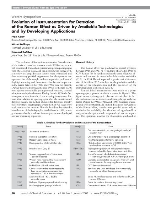
Raman’s initial measurements were made on a prism 

spectrograph, a picture of which is shown in Figure 1. This 

figure shows a photographic plate on the exit, but, in fact, 

the earliest measurements were made using the eye as the detector. 

During the 1930s, 1940s, and 1950s hundreds of compounds 

were synthesized and studied. Because of the weakness 

of the Raman effect, samples were purified extensively to 

maximize the probability that the observed signal could be 

assigned to the synthesized compound and not to impurities. 

The equipment used for the observations was based on 

Year(s) 

Table 1. Timeline for the Prediction and Discovery of the Raman Effect 

E vent 

Year(s) 

1922–1927 

MTheoretical 

predictions 

1971 

Event 

MFirst 

instrument with concave gratings introduced 

MMby 

Jobin Yvon 

1928 

MRaman’s 

publication in 

Nature 

1972 

MCharacteristics 

of triple spectrograph described 

1934 

MPlaczek’s 

semi-classical theory 

1973 

MHirschfeld 

predicted femtoliter sampling 

1939 

MDevelopment 

of photomultiplier tube 

1974 

MNBS 

described Microprobe at ICORS; Jobin Yvon 

MMexhibited 

the prototype MOLE 

1953 

MIntroduction 

of Cary 81 

1980–1985 

MTriple 

spectrographs with multichannel detectors 

MMcommercialized 

by Spex, Jobin Yvon, and Dilor 

1961 

MTownes 

suggested use of HeNe laser 

MMas 

Raman source 

1964 

MWeber, 

Porto reported first measurement 

MMwith 

ruby and HeNe lasers 

1985 

MBruce 

Chase and John Rabolt demonstrated 

M MFT–Raman 

systems with Nd:YAG laser (1064 nm) 

1990 

MCarrabba 

demonstrated holographic filter with small 

MMmonochromator 

for acquiring Raman spectrum 

1964 

MPerkin 

Elmer LR1 with HeNe laser 

1991 

MCCD detectors introduced 

1965 

MCary 

81 converted to accommodate the 

MMlaser 

as excitation source; recorded 

MMs pectrum of 0.25 

µ L-benzene sample 

1965 

MSpex 

introduced 1401, double 

MMmonochromator 

1992 

MRenishaw and Dilor introduced first commercially 

MMsuccessful 

benchtop Raman systems 

1993 

MStable 

785-nm laser source and red-enhanced CCD 

MMfor 

near-IR Raman 

1966 

MDelhaye, 

Migeon proposed microfocusing 

1994 

MPatent 

for confocal line-scanning issued 

1968 

MFirst 

holographic gratings produced 

2002 

MCombination 

Raman, FT–IR system introduced at Pittcon 

50 Journal of Chemical Education • Vol. 84 No. 1 January 2007 • www.JCE.DivCHED.org


Figure 1. Photograph of Raman’s spectrograph from the archives 

of the Indian Association for the Cultivation of Science, Jadavpur, 

Kolkata; provided by D. Mukherjee. 

Figure 3. Steinheil Raman spectrometer, shown without the associated 

electronics, which filled two full-height racks. 

large, high-index prisms, and photographic plates. Early 

workers from Jobin Yvon (10) reported using high-aperture 

lenses to maximize luminosity. The spectra were first generated 

by filtered sunlight and later mercury arc lamps filtered 

to pass the excitation line. Because of the long integration 

times (tens of hours) any particles in the sample would produce 

flashes of light that would ruin the plates. Therefore 

the purification process also included filtering. The plates 

were heated to increase their sensitivity to light, which resulted 

in the term “baked plates”. 

Curiously, until the mid 1940s there was much more 

activity in Raman spectroscopy rather than infrared (IR) absorption 

because of the relative ease of the Raman measurements 

over the IR during that period. There were 

manufacturers of these prism instruments in France (Huet), 

the United Kingdom (Hilger and Watts), Germany 

(Steinheil), and Russia (unknown). These instruments were 

often totally integrated with lamp and detector. After the introduction 

of photomultiplier tubes (PMTs) in the late 1930s 

(11), these detectors were sometimes offered as an alternative 

to the photographic plate. 

The availability of high-index glass provided good dispersion 

in the prisms, which could be quite large. Sometimes 

a large lens was mounted quite close to the photographic 

plate, which provided a high flux on the photographic plate, 

all for optimized sensitivity. The dispersion of a prism does 

not exhibit an analytical function. Its wavelength calibration 

was achieved by measuring well-known lines of an atomic 

lamp. Figure 2 shows three spectrographs from Huet and a 

Raman spectrum superimposed on spectra of the mercury 

and iron arc lamps. The extraction of frequency shift values 

from these plates was a tedious process. Figure 3 shows the 

Steinheill system that utilized three medium-sized prisms (ca. 

3–4 cm). This system used both high- and low-pressure mercury 

arc lamps, and a PMT detector. The slit and PMT were 

scanned across the focal plane. Collimator and camera mirror 

focal lengths could be changed to select the dispersion of 

interest. Figure 4 shows the optical layout of a two-prism spectrograph 

from Hilger and Watts. This instrument shows both 

a camera and a PMT. In this system a scanning mirror returned 

the light from the spectrograph back to the entrance 

where a slit was mounted. As the angle of the mirror was 

Figure 2. Product literature showing the Huet prism spectrographs, 

and a photographic plate with spectral lines from the mercury arc, 

an iron arc, and the Raman spectrum itself. 

Figure 4. Optical layout of two-prism Hilger and Watts spectrograph, 

shown with a slit and scanning mirror system to be used 

with a PMT. 

www.JCE.DivCHED.org • Vol. 84 No. 1 January 2007 • Journal of Chemical Education 51


Figure 5. Photograph of full Hilger and Watts system. 

Figure 7. A spectrum of benzene (0.25 µL), ecited at 4358 Å, recorded 

at 10 cm 1 resolution in about 5 minutes with the Toronto 

arc source. 

Figure 6. Optical layout of Cary 81, with a Toronto arc lamp. 

scanned, the wavelength passing through the slit was changed, 

and the signal was detected by the PMT. This system was 

designed in collaboration with Menzies, an advisor to Hilger 

and Watts. Figure 5 shows the entire system from Hilger and 

Watts. One can argue that this was an early, fully integrated 

“table top” system. 

The Middle Period: 1950s–1970s 

Electronics for single photon counting on PMTs was 

introduced (12). This meant that, given the optical signal 

detected, all components of noise were eliminated except for 

the statistical component inherent in the counting of the 

photon events itself. 

Prism-based instruments were replaced with gratingbased 

instruments, which have the following positive characteristics: 

• Good efficiency 

• High angular dispersion, with better performance in red 

• Analytical description of dispersion, which simplified 

wavelength calibration 

• Large useful area 

Double monochromators were built to minimize stray 

light; their lower efficiency was offset by larger slits that could 

be used for equivalent resolution. In addition, inteferometric 

control was introduced in about 1955 reducing grating ghosts 

and stray light. 

Townes, the inventor of the laser, first suggested the use 

of the HeNe laser as a Raman source in 1961 (13). The first 

measurements of Raman spectra excited by the HeNe laser 

were reported by Weber and Porto (14). As soon as the argon 

and krypton ion gas lasers were introduced, these lasers 

were also exploited as Raman sources. 

The Cary 81 Raman spectrometer was the first “easyto-use” 

system. People reported being able to record spectra 

as soon as the instruments were delivered to their laboratories. 

The instrument was introduced at the Molecular Spectroscopy 

Conference in Ohio in 1954. It used a 3 kW helical 

Toronto Hg arc, water-cooled for low background, and low 

pressure for sharp excitation lines. The monochromator was 

a Czerny–Littrow double, with 1200 gmm gratings, 1 that 

was mechanically scanned at speeds between 0.0005 to 50 

cm 1 s. There were many innovations implemented to optimize 

its performance: 

• Multi-slit design 

• Reference phototube 

• Plano convex lenses to correct for slit curvature and 

to reduce aberrations 

• The signal was chopped between two PMTs and recombined 

to recover the lost signal from chopping. 

• An image slicer was designed to recover signal lost at 

the entrance slit when the slit was significantly overfilled 

by the sample image. 

Figure 6 shows the optical layout of the Cary 81 equipped 

with the Toronto arc, and Figure 7 shows a spectrum representative 

of its performance. The Cary system was retrofitted 

with a HeNe laser in 1964 and renamed the Cary 82. 

Perkin–Elmer produced the first “benchtop” system in 

1966, integrating the laser as a source. It was based on a 

double-pass monochromator previously used to record infrared 

spectra. A multipass sample cell was also introduced. 

Other multistage grating monochromators built during this 

period are listed in Table 2. 

Spectrometer and Spectrograph Design 

Grating spectrometers and spectrographs come in several 

design types. The design is based on several goals. When 

the signal is detected with a PMT mounted behind an exit 



Table 2. Scanning Monochromators with PMTs 

Year 

Company 

1953 

Cary 

91 

1964 

Cary 

82 

1964 

Spectra 

Physics 

1964 

Steinheil 

1966 

Perkin–Elmer 

1967 

Spex 

1967 

Coderg 

1968 

Jarrell 

Ashe 

1972 

Coderg 

1972 

Jobin Yvon 

Type 

Double 

Additive CT 

Double 

Additive CT 

Double 

Additive Ebert 

Double Additive lenses 

Double Additive CT 



Double Subtractive CT 

Triple Additive SR 

Double Additive 

concave gratings 

Light Source 

Hg Toronto lamp 

HeNe laser 

HeNe 

NO TE: CT is Czerny–Turner and SR is Sergent-Rozey. 

slit, it is desirable to transfer a tight focus to the slit to maintain 

optimal spectral resolution. In addition, it is necessary 

to minimize stray light. The most common spectrometer design 

is called a Czerny–Turner (15), which was created to 

minimize lowest-order coma, one of the primary optical aberrations. 

An alternative design to the Czerny–Turner, the 

Sergent-Rozey (16, 17), has been used on several occasions 

Figure 8 shows the principle governing these two designs. The 

circle surrounding the grating is the locus of points that minimizes 

aberrations. For a grating mounted with its grooves 

vertical, as shown in the figure, slits can be placed along a 

line transecting the grating either in the horizontal plane or 

the vertical plane. The tilt of the concave mirrors is then adjusted 

to correctly send the light through the system. A 

Czerny–Turner monochromator uses slits along the horizontal 

trace, whereas the Sergent-Rozey uses the slits along the vertical 

line. 

The Sergent-Rozey system has two advantages that are not 

well recognized. In the first place spectral anomalies due to 

re-diffracted light are totally eliminated. The figure shows the 

artificial spectra in the two designs. In the Czerny–Turner design 

parts of the spectrum focused by the camera mirror on 

the slit plane can potentially fall on the grating to be re-diffracted 

somewhere through the system causing artifacts in the 

spectrum. In the Sergent-Rozey design the final spectrum is 

focused below the grating where it would not be re-diffracted. 

The second characteristic becomes important when designing 

multistage systems. A double Sergent-Rozey monochromator 

can be made by mounting the two gratings side-by-side 

on a single shaft. In that case, no additional mirrors are required 

to direct the light from one monochromator to the next. 

This is illustrated in Figure 9 that shows the layout of the T800, 

which was actually a triple spectrometer. However, the disadvantage 

of this design was that it takes up more volume. Further 

modifications were made to the Czerny–Turner design to 

optimize it for use with multichannel detectors. Ray tracing 

indicated that asymmetrization would sharpen the slit image 

(18), and flatten the focal surface (19). 

In 1966, the first holographic gratings were produced 

using photoresist that was exposed to interfering laser beams. 

Holographically recorded gratings have the advantage that 

they eliminate essentially 100% of the ghosts and stray light 

artifacts of conventionally ruled gratings. Figure 10 shows 

laser reflection patterns from two gratings of the same groove 

Figure 8. Principle of Czerny–Turner vs Sergent-Rozey spectrometer 

design. The Czerny–Turner plane is horizontal in this figure 

while the Sergent-Rozey is vertical. 

Figure 9. Optical layout of T800, a triple scanning spectrometer 

of the Sergent-Rozey design: s = slit and G = grating. 

Figure 10. Laser diffraction patterns from conventionally ruled and 

holographic gratings. 



density. The bright spots are diffraction orders. Between and 

around the diffraction spots from the conventionally ruled 

grating is a significant quantity of light due to imperfections 

in the grating. The improvement in performance of holographic 

gratings has the potential for much improved stray 

light rejection in Raman spectrometers and spectrographs. 

Figure 11 shows the optical layout of the HG2S, the first 

Raman spectrometer based on holographically recorded gratings. 

This instrument was introduced in 1971. It was neither 

a Czerny–Turner nor a Sergent-Rozey. It used concave 

gratings. It was not necessary to have any optics other than 

the gratings between the slits. Consequently there were no 

additional sources of stray light. The low frequency performance 

of this instrument was significantly improved over 

anything that preceded it. Spectra could be recorded to frequency 

shifts lower than 10 cm 1 . Figure 12 shows the very 

low frequency spectrum of SiO 2 . 

Before the use of computers, spectra were scanned synchronously 

with strip chart recorders. Most spectrometers 

have drive systems where linear movement of a stepper motor 

is related to the wavelength diffracted by the grating. 

However, the Raman spectrum is described naturally in terms 

of shifts in the reciprocal of the wavelengths. That meant that 

a different drive system evolved for Raman instruments. The 

diffraction equation relating the incident and scattered angles 

i and i, to the wavelength of light is 

sini + sini′ = knλ 

where k is the diffraction order and n is the index of refraction 

(= 1 in air). Simple geometric arguments indicate how it 

is possible to devise a mechanical system that can scan in cm 1 

rather than nm. This is illustrated in Figure 13. The grayshaded 

triangles represent the triangles that get pushed by linear 

motion from a motor and that motion is related in a linear 

fashion to either the sine or cosecant of the included angle. 

Multichannel Detectors 

The development of reliable multichannel detectors in 

the early 1980s meant that Raman spectra could again be 

collected in the same “multiplexed” fashion as had been used 

with the photographic plate, but now with all of the advantages 

of an electronic detector in terms of signal-to-noise, 

wavelength response, dynamic range, and digital storage and 

manipulation. The earliest detectors were the intensified photodiode 

array and the imaging PMT. The imaging PMT had 

good noise characteristics but limited dynamic range. The 

photodiode array was the detector of choice for commercial 

instruments for years until the maturation of the high sensitivity 

of the CCD camera. It inherently provided lower noise, 

and the wavelength sensitivity was not limited to the photocathode 

of the image intensifier. In addition, it was two-dimensional 

with the important implication that Raman 

mapping and imaging had new possibilities. 

With the introduction of these detectors, it became clear 

that the Raman spectrograph needed a total new design to better 

match the detector size. A typical device had 1000 25 µm 

pixels, but the coverage on the detector from a double monochromator 

(which only provided a 18-mm unvignetted field) 

was about 150 cm 1 when the 1800 gmm gratings were used 

with an argon laser. In addition, the low frequency performance 

was significantly degraded when an exit slit with PMT was 

replaced by larger intermediate slits and a multichannel detector 

in the focal plane. 

The instruments designed specifically to be used with 

multichannel detectors first included a double subtractive 

premonochromator to filter the laser beam (20). The focal 

length and grating groove density of the dispersive stage were 

selected so that the final coverage was about 1000 cm 1 , or 1 

pixelcm. The stray light properties of this design were analyzed 

carefully in the Ph.D. thesis of Michel Leclercq at the 

University of Lille (21, 22). Several commercial products have 

been produced since 1979 and are shown in Table 3. When 

calibrating spectra on a multichannel array, in principle the 

wavenumber shift at every pixel can be predicted from the 

focal length, groove density, and pixel size, once the central 

Figure 11. Optical layout of HG2S based on concave holographic 

gratings. 

Figure 12. Brillouin spectrum of SiO 2 showing bands at ±0.8 cm 1 . 

Figure 13. Trigometric description of the cosecant and sine drives— 

x represents the linear motion of the motor which is converted to 

angular motion of the grating in units linear with the sine or cosecant 

of the angle. 



Commercial 

Product 

Table 3. Commercial Raman Instruments with Multichannel Detectors 

Year 

of Introduction 

Description 

Configuration 

2 

OMARS89 

1979 

M ultichannel and single channel 

( 0.5 m) 

(0.4 m/0.3 m) 

2 

1877 

1981 

8 -mm intermediate slit, limited coverage 

( 0.34 m) 

(0.5 m) 

MICRODIL28 

1981 

Confocal laser scanning microscope, (lenses in 

3rd stage), patented lens-scanning system 

3 

( 0.5 m) 

2 

S3000 

1985 

---- 

( 0.32 m) 

(0.64 m) 

3 

XY 

1986 

M odular, additive mode, SAS*, csc drive 

( 0.5 m) 

r (0.8 m) 

o 

3 

2 

Jasco 

~ 19870 ---- 

( 0.64 m) 

(0.64 m) 

2 

T64000 

1988 

A dditive mode, SAS, sine drive 

( 0.64 m) 

(0.64 m) 

Acton 

2000 

Modular 

---- 

NO TE: SAS means that Stokes and anti-Stokes measurements can be made simultaneously. 

pixel is known. Figure 14 illustrates the calculations used to 

generate this information (23). It is important to realize that 

the choices in spectrograph focal length, groove density, and 

pixel size that will be used with a given laser wavelength will 

determine not only spectral coverage but also resolution, and 

that resolution cannot be improved beyond the equivalent 

dispersion in two pixels on the CCD. This resolution will 

only be achieved with the entrance slit is set to a value between 

one and two pixels wide. However, on these systems 

the resolution and coverage can be optimized for a particular 

measurement by selecting a grating from a number of 

choices. 

Figure 15 shows single shot spectra recorded from polycrystalline 

graphite using two different gratings (1800 gmm 

vs 600 gmm) and two different laser wavelengths (632.817 

and 514.532 nm). The focal length of the system used for 

these measurements (LabRAM) was 300 mm. The differences 

in dispersion and coverage are clear. Note that the number 

of cm 1 Å in the green are about 4 but about 6 in the red. 

Since the dispersion in Å of a spectrograph is relatively constant, 

the resolution differences noted between the spectra 

acquired with the two lasers using a given grating is due principally 

to the number of cm 1 Å at the two laser wavelengths. 

resolution of the final spectrum. Figure 16B illustrates how 

this was implemented on the T64000. This instrument has 

an optical option that can convert the subtractive 

premonochromator into an additive one. In this case, one can 

record spectra in both additive and subtractive modes—in one 

case for high resolution and in the other for high stray light 

rejection. The spectra reproduced in Figure 17 were recorded 

from a semiconductor superlattice. Bands down to 4 cm 1 are 

clearly visible. These very low frequency bands have been recorded 

with a CCD using the system in subtractive mode and 

with a PMT in additive mode. 

Raman Microscopy 

The Raman community initially exhibited very little interest 

in Raman microscopy. It was argued that because the 

Raman signal scales with the number of exciting molecules, 

reducing the sample size would produce unacceptably weak 

signals. In 1966, Delhaye and Migeon published calculations 

Triple Spectrographs 

The principle of a classical triple spectrograph (double 

subtractive + spectrograph) is illustrated in Figure 16A. The 

premonochromator presents non-dispersed, but laser-filtered 

light to the spectrograph stage whose dispersion defines the 

Figure 14. Raman shift calculation for a multichannel detector. 

Figure 15. Raman microprobe spectra of polycrystalline graphite 

recorded on the LabRAM using laser lines at 514.532 and 632.817 

nm and gratings with 600 and 1800 g/mm groove density. 



(24, 25) that showed that the loss of signal would be fully compensated 

by the advantages of a microprobe, which include 

• Tight laser focus at sample (resolution ∼1 µm) 

• Raman collection efficiency 

• Effective coupling of the sample volume on a small 

entrance slit. 

[According to Delhaye the only Raman researcher who 

showed an interest was Tomas Hirschfeld, but because of his 

involvement with the military, little of his work had been 

published with one exception (26).] 

It was only in 1973 when Raman microscopy was proven 

simultaneously in two locations. Paul Dhamelincourt, then a 

student of Delhaye, assembled a system that proved that a 

Raman microscope really was feasible. The initial experiments 

in Delhaye’s laboratory showed that it was possible to record 

a picture of a sample through its Raman light. Subsequently 

spectra of microparticles were measured. Simultaneously Greg 

Rosasco and Edgar Etz at the National Bureau of Standards 

assembled a microprobe based on an elliptical reflector in order 

to study environmental microparticles. The first publications 

documenting these experiments appeared in the abstracts 

for the Raman spectroscopy conference in 1974 (27, 28). 

Delhaye and Dhamelincourt (29) described their imaging 

Raman concepts in a publication in 1975 where they 

A 

showed several possibilities for creating a Raman image. These 

possibilities are illustrated in Figure 18. Based on these concepts 

the first commercial instrument, the MOLE, was introduced 

in 1974. The prototype is shown in Figure 19. 

This instrument had three modes of operation. It was 

based on a double monochromator using 1 m concave holographic 

gratings. When used as a microprobe, a 1-µm laser 

spot was imaged onto the entrance slit and then onto a PMT. 

When used as a spectrograph, a SIT or SEC camera was 

mounted at the exit focal plane and a range of about 100 cm 1 

could be viewed for kinetic measurements. When used as a 

Raman microscope, the sample was illuminated globally and 

it was imaged onto the grating rather than the slit. The image 

of the sample, after being diffracted by the grating, was 

projected onto the camera. Figure 20 shows the results of these 

three modes of operation on a mixture of MoO 3 and K 2 CrO 4 . 

Raman Microprobe 

The success of a Raman microprobe is based on four 

optical properties: 

• Laser focal spot at the sample 

• Collection efficiency of the microscope optics 

• Efficiency of the coupling of the light coming from 

the laser focal volume and the spectrometer or spectrograph 

• Confocal principle 

B 

Figure 16. (A) Principle of triple Raman spectrograph with double 

subtractive foremonochromator. (B) Optical layout of T64000 in subtractive 

mode. Because of the reversal of the sense of dispersion of 

gratings G 1 and G 2 , the slit S 3 sees nondispersed light that has been 

filtered by the foremonochromator. The coverage is determined by 

the size of the slit S 2 , which can be as large as 50 mm. 

Figure 17. (A) SiGe superlattice spectrum recorded on T64000 

working in subtractive mode with a CCD detector. (B) SiGe 

superlattice spectrum recorded on T64000 working in additive 

mode with PMT. Note that the ultimate low frequency performance 

is achieved in this mode of operation. 



The Raman microprobe is based on the recognition of the 

focusing properties of high numerical aperture (NA) objectives. 

The beam spot size w, of a laser beam entering a wellcorrected 

objective is 

ω 

≈ 

λ 

NA 

This equation indicates that the spot size decreases as the 

wavelength of the radiation decreases and as the NA increases. 

For visible radiation and 100× objectives (NA > 0.9), it is 

easy to achieve spot sizes under 1 µm. 

The collection efficiency is also determined by the NA 

of the objective. Good, high NA microscope optics far exceed 

even the best macro Raman sampling optics. Figure 21 

shows the results of calculations illustrating this point. Figure 

22 shows the principles of the scheme to transfer the Raman 

light collected by the objective to the entrance slit. Not 

only is the laser focal volume at the sample imaged on the 

entrance slit (and later on the detector), but the back aperture 

of the objective is imaged onto the grating, the limiting 

aperture of the spectrograph. For this reason multiple lenses 

are used in the optical train. The top of the figure illustrates 

this principle; the bottom part of the figure illustrates its 

implementation. Note that between the microscope and the 

spectrograph there is an intermediate image plane at which 

is mounted a hole that is “confocal” to the sample and the 

entrance slit. The principles for this coupling was described 

in a publication by Dhamelincourt (30). 

Figure 20. Three modes of operation of MOLE. Upper left shows a 

white light image. The two lower left images show Raman micrographs 

in lines of MoO 3 and K 2 CrO 4 . Upper right shows the spectrum 

of the chromate species on the multichannel detector and the 

lower right shows the PMT output of the same spectrum. 

O PTIC 

NA 

= nsinθ 

n = 1 n = 1.33 

n = 1. 5 θ Ω/2π 

f/ 10 

0.0499 

0.066 

0.74 

2.862 

0.06 

f/ 5 0.099 

0.131 

0.148 

5.71 

0.25 

f/ 4 0.124 

0.165 

0.186 

7.125 

0.38 

f/ 3 0.164 

0.218 

0.246 

9.462 

0.68 

10x 

f/ 1.93 

0.25 

0.332 

0.375 

14.477 

1. 5 

M Chamber f/ 1. 8 0.267 

0.355 

0. 

4 15.485 

1. 8 

M Chamber2 f/ 1. 4 0.336 

0.447 

0.504 

19.633 

2. 9 

20x 

ULWD f/ 1.14 

0. 

4 0.532 

0. 

6 23.578 

4. 1 

f/ 1 

0.44 

0.594 

0.67 

26.551 

5. 2 

50xULWD 

f/ 0.75 

0.554 

0.737 

0.831 

33.69 

8. 4 

50x 

f/ 0.44 

0.75 

0.997 

1.125 

48.59 

16. 9 

100x 

f/ 0.164 

0.95 

1.263 

1.425 

71. 

8 34. 3 

Figure 18. Various schemes for Raman imaging. (Reproduced with permission: 

Delhaye, M.; Dhamelincourt, P. J. Raman Spectrosc. 1975.) 

Figure 19. Prototype MOLE Raman microscope. 

Figure 21. Top: Tabulation of relationship between f/#; NA; collection 

efficiency, Ω/2π; and θ, the included half angle of the optic. 

Bottom: Definition of optical angle θ and collection efficiency, 

Ω/2π. Note that f/1 corresponds to 26°, but its collection efficiency 

is about 1 /4 that of a 100× microscope objective. 



Figure 22. (Top) Optical principle describing how light is collected 

and imaged from the Raman volume to the spectrograph. (Bottom) 

Implementation of this principle. Note the pinhole spatial filter that 

will serve as a confocal hole for increased spatial resolution. These 

figures are reproduced from Figures 9 and 10 of ref 31. 

The principle of confocality is described in Figure 23. 

The idea is that insertion of an aperture in a plane conjugated 

to the plane of analysis will block Raman radiation 

emitted by material surrounding the laser-irradiated volume. 

This has the effect of assuring that the Raman spectrum represents 

the material of interest, as well as blocking fluorescence 

and Rayleigh light. The degree of confocality will be 

determined by the size of this hole relative to the size of the 

image, as well as the NA of the microscope optics. 

The early 1990s saw the development of a method to 

map samples confocally while multiplexing the laser beam 

on the sample and taking advantage of the second dimension 

of the CCD (32). The principle is shown in Figure 24. 

The laser is scanned across the back aperture of the objective 

in such a way as to avoid introducing aberrations and 

then losing the diffraction limit in the laser spot. The Raman 

light returns on the same scanning mirror so that it 

can be then focused through the confocal hole and rescanned 

onto the entrance slit of the spectrograph. Each 

point on the slit represents Raman signal from a confocally 

defined spot on the sample. By appropriately processing the 

signal on the CCD, one can construct a Raman map that is 

truly confocal. 

While certainly Raman micrographs can be recorded directly 

as was shown earlier, the confocal mapping provides 

significant advantages to these capabilities. Raman signals tend 

to be weak and are easily overwhelmed by background signals. 

In the case of microscopy, this can be matrix signals (i.e., 

from material around the directly illuminated spot) as well 

as luminescence and Rayleigh light. Confocal aperturing reduces 

most of these unwanted signals so that the resulting 

Raman images have much better contrast. While sometimes 

it is possible to subtract these background levels, subtraction 

will never remove the noise created by high background levels. 

Figure 25 shows the results of a confocal map of a histological 

section containing Dacron (polyethylene terephthalate) 

fibers with adhering protein. Note that this map was performed 

with a HeNe laser on a “real-world” sample. 

Figure 23. Principle of confocality: only light being emitted from 

the focal plane of the instrument will be efficiently transmitted by 

the confocal aperture and onto the detector. These figures are reproduced 

from Figures 11 and 13 of ref 31. 

Figure 24. Optical scheme for confocal line-scanning. Reproduced 

from Figure 7 of ref 38. 



The Current Period 

Several technologies have been important for the rapid 

increase in Raman use over the past decade. They include 

• Multichannel detectors 

• Air-cooled lasers 

• Desktop computers 

• Holographic notch filters 

The one item on this list that is most specific to Raman instrumentation 

is the holographic notch filter. Carrabba (33) 

made the first measurements with this class of filter and 

showed that it would no longer be necessary to use large instruments 

for many routine Raman measurements. The 

physical principles of volume holography were laid out in 

1993 (34) and will certainly be covered in detail in Harry 

Owen’s contribution. 

However, there is an historical curiosity that has come 

to our attention. In a 1948 publication in France, J.-L. 

Delcroix reported the use of “Lippman plates” as filters (35). 

Gabriel Jonas Lippman had received the Nobel Prize in 1908 

for “for his method of reproducing colors photographically 

based on the phenomenon of interference”. The Lippmann 

reflection filters were based on gelatin, with silver films on 

them, and a mercury layer assuring reflection. Delcroix notes 

that these filters can reflect a particular wavelength (which 

will depend on the angle of incidence) but transmit all others. 

To quote him “En particular, Mr. Kastler avait en l’idee 

d’utiliser les plaques Lippmann, dans l’obtention des specters 

Raman, pour affaiblir la raie excitatrice si genante dans 

l’etude des raies de basses frequencies.” (In particular, Mr. 

Kastler had the idea to use the Lippmann plates in order to 

obtain Raman spectra, by reducing the exciting ray that is 

troublesome in the low frequency region.) 

Figure 25. Confocal map of Dacron fibers in histological section: 

proteins appear green, fibers appear red, and the proteins that 

overlay the fibers appears yellow. A color version of this image is 

located in the table of contents. 

Benchtop Instruments 

Figure 26. Schematic of proposed implementation of a Raman microprobe 

in an electron microscope. Figures from ref 37, p 164. 

Following the recognition that the notch filter could enable 

the construction of Raman instruments of vastly reduced 

size, benchtop instruments appeared on the market. Because 

of their reduced complexity, much less light was lost in the 

optics and much more reached the detector. The CCD, a 

multichannel detector with extremely low noise became the 

detector of choice. Spectra could now be recorded in seconds 

to minutes instead of hours. Highly powerful desktop computers 

made instrument control and data treatment very sophisticated. 

Systems really can be turn-key and easy-to-use. 

The availability of long wavelength red lasers (785 or 

830 nm) provides almost fluorescence-free results for “dirty” 

organic materials. UV optics are now available for UV Raman 

microscopy, and its application is certain to have an 

impact in semiconductor studies. However, application of 

these systems is sometimes limited by laser-induced photochemistry, 

especially of organic materials so the universal usefulness 

may not be achieved. 

Near-field micro-spectroscopy (36) is certainly a field 

that is showing some interest, but whether there is sensitivity 

for a true near-field Raman signal is in controversy. Conversations 

both with Aaron Lewis of Nanonics and Bruce 

Chase of DuPont have indicated that the sensitivity is not 

adequate. What can be useful, however, is the ability to identify 

a good region for analysis and then to do the Raman 

microanalysis in the far field. 

Another area that has shown some interest is the integration 

of a Raman probe with an electron microscope (Figure 

26). This is interesting because Delhaye’s original interest 

in the Raman microprobe was generated by his interaction 

with Castaing and the developing electron microprobe of the 

time. Delhaye has proposed that elliptical reflectors could be 

introduced in an electron microscope at the sampling point 

and coupled to a laser and Raman spectrometer (37). 



Closing Remarks 

Certainly when reviewing the evolution of Raman instrumentation, 

one is struck by the cycling of many concepts. 

The first instruments were prism-based spectrographs using 

lenses for collimation and focusing. Today’s instruments are 

also spectrographs, but they use CCD cameras instead of photographic 

plates. While mirror-based spectrometers were used 

almost exclusively in the middle period, benchtop instruments 

working in the visible today use lenses with their superior 

focusing properties. There is of course no analog to the laser 

source in the earlier instruments. But the real surprise in researching 

this article was the discovery that the Lippmann 

filter technology, which appears to be a pre-laser replica of 

today’s holographic filters, was suggested as a means to suppress 

the source scattering in a Raman spectrum. The major 

difference, that the holographic filters are produced with lasers, 

affords superior control of the production of the filters. 

The take-home message is that many of the ideas that make 

the current instruments so successful were tried at various times 

over the previous 80 years. But all these technologies converge 

today to produce the quality of instrumentation that has shown 

such promise for the future of materials analysis. 

Acknowledgments 

The authors wish to thank the following for helpful discussions 

in preparation of this manuscript: Michael Carrabba, 

Paul Dhamelincourt, John Ferrarro, Michel Leclercq, Joel 

Oswalt, Anant Ramdas (Raman’s last student), Hans Juergen 

Reich, Bernard Roussel, Steve Slutter, Alfons Weber, and 

Andrew Whitley. 

Note 

1. Grooves per millimeter is expressed as g/mm. 

Literature Cited 

1. Raman, C. V. Proc. R. Soc. London, Ser. A 1922, 101, 64. 

2. Smekal, A. Naturwissenschaften 1923, 11, 873. 

3. Kramers, H. A.; Heisenberg, W. Z. Phys. 1925, 31, 681. 

4. Schroedinger, E. Ann. Phys. 1926, 81, 109. 

5. Dirac, P. A. M. Proc. R. Soc. London, Ser. A 1927, 114, 710. 

6. Raman, C. V. Nature 1928, 121, 501. Ind. J. Phys. 1928, 2, 387. 

7. (a) Rocard, Y. Comptes Rendus Acad. Sci. 1928, 186, 1107– 

1109. (b) Cabannes, J. Comptes Rendus Acad. Sci. 1928, 186, 

1201–1202. 

8. Landsberg, G.; Mandelstram, L. Naturwissenschaften 1928, 16, 

557, 772. 

9. Placzek, G. Rayleigh-Streuung und Raman-Effekt. In 

Handbuch der Radiologie; Marx, E., Ed.; Academische-Verlag: 

Leipzig, Germany, 1934; Vol. VI.2, p 205. 

10. Daure, M.; Cabannes, M. Rev. Optique, Theorique Instrum. 

1928, 7, 450–456. 

11. Zworykin, V. K.; Rajchman, J. A. Proc. Inst. Radio Eng. 1939, 

27, 558–566. 

12. Morton, G. A. Appl. Opt. 1968, 7, 1–20. 

13. Townes, C. H. In Advances in Quantum Electronics; Singer, J. 

R., Ed.; Columbia University Press: New York, 1961; pp 3–11. 

14. Weber, A.; Porto, S. P. S. J. Opt. Soc. Am. 1965, 55 (8), 1033–1034. 

15. Czerny, M.; Turner, A. F. Z. Phyzik. 1930, 61, 792. 

16. Sergent-Rozey, M. Rev. Optique 1965, 44, 193–203. 

17. Arie, G.; Lescouarch, J. Cl.; Demol, R. Nouv. Rev. Optique 

Appliquee 1972, 3 (5), 281–284. 

18. Shafer, A. B.; Megill, L. R.; Droppleman, L. J. Opt. Soc. Am. 

1964, 54, 879–887. 

19. Reader, J. J. Opt. Soc. Am. 1969, 59 (9), 1189–1196. 

20. Grayzel, R.; Leclercq, M.; Adar, F.; Hutt, M.; Diem, M. An 

Automated Micro–Macro Raman Spectrograph System with 

Multichannel and Single-Channel Detectors in a New Molecular/Crystalline 

Microprobe. In Microbeam Analysis; 

Armstrong, J. T., Ed.; San Francisco Press: San Francisco, 

1985; pp 19–25. 

21. Leclercq, M. Etude de Premonochromateurs Soustractifs et de 

Spectrometers Raman a Reseaux Holographiques Concaves. 

Ph.D. Thesis, L’Universite des Sciences et Techniques de Lille, 

Lille, France, 1975. 

22. Leclercq, M.; Walart, F. J. Raman Spectrosc. 1973, 1, 578–593. 

23. Katzenberger, J. M.; Adar, F.; Lerner, J. M. An Improved Algorithm 

for Linearizing in Wavelength or Wavenumber Spectral 

Data Acquired with a Diode Array. In Microbeam Analysis; Geiss, 

R. H., Ed.; San Francisco Press: San Francisco, 1987; p 165. 

24. Delhaye, M.; Migeon, M. C. R. Acad. Sc. Paris 1966, 262, 

702–705. 

25. Delhaye, M.; Migeon, M. C. R. Acad. Sc. Paris 1966, 262, 

1513–1516. 

26. Hirschfeld, T. J. Opt. Soc. Am. 1973, 63, 476. 

27. Rosasco, G. J.; Etz, E. Investigation of the Raman Spectra of 

Individual Micron Sized Particles. In Proceedings, Fourth International 

Conference on Raman Spectroscopy, Brunswick, 

ME, Aug 25–29, 1974; Abstract 5.1.10. 

28. Delhaye, M.; Dhamelincourt, P. Laser Raman Microprobe and 

Microscope. In Proceedings, Fourth International Conference 

on Raman Spectroscopy, Brunswick, ME, Aug 25–29, 1974; 

Abstract 5.B. 

29. Delhaye, M.; Dhamelincourt, P. J. Raman Spectrosc. 1975, 3, 

33–43. 

30. Dhamelincourt, P. Instrumentation and Recent Applications 

in Micro Raman Spectroscopy. In Microbeam Analysis; 

Heinrich, K. F. J., Ed.; San Francisco Press: San Fancisco, 

1982; pp 261–269. 

31. Turrell, G.; Delhaye, M.; Dhamelincourt, P.; Characteristics 

of Raman Microscopy. In Raman Microscopy; Turrell, G., Corset, 

J., Eds.; Academic Press: London, 1996; Chapter 2. 

32. Delhaye, M.; DaSilva, E.; Barbillat, J. European Patent No. 

92400141.5, 1992. 

33. Carrabba, M.; Spencer, K. M.; Rich, C.; Rauh, D. Appl. 

Spectrosc. 1990, 44, 1558–1561. 

34. Tedesco, J. M.; Owen, H.; Pallister, D. M.; Morris, M. D.; 

Anal. Chem. 1993, 65, 441A–449A. 

35. Delcroix, J.-L. Rev. Optique 1948, 27 (8–9), 493–509. 

36. Harootunian, A.; Betzig, E.; Isaacson, M.; Lewis, A. Appl. Phys. 

Lett. 1986, 70, 1671. 

37. Truchet, M.; Delhaye, M. Transmission Electron Microscope 

with Castaing’s Electron X-ray and Laser Raman Probes for 

Simultaneous Elemental and Molecular Analysis at 

Submicrometric Scale. In Microbeam Analysis; Geiss, R. H., 

Ed.; San Francisco Press: San Francisco, 1987; pp 163–164. 

38. Barbillat, J. Raman Imaging. In Raman Microscopy; Turrell, G., 

Corset, J., Eds.; Academic Press: London, 1996; Chapter 4.

History of Raman Technology Development - Academic Program ...

You also want an ePaper? Increase the reach of your titles

Delete template?

Save as template?