HiCIRF: A highfidelity HF channel simulation - Digital Library
HiCIRF: A highfidelity HF channel simulation - Digital Library
HiCIRF: A highfidelity HF channel simulation - Digital Library

Create successful ePaper yourself
Turn your PDF publications into a flip-book with our unique Google optimized e-Paper software.
RS0L11<br />
NICKISCH ET AL.: HICIRF <strong>HF</strong> CHANNEL SIMULATION<br />
RS0L11<br />
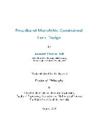
Figure 1.<br />
Sample receiver array geometry.<br />
suitable corresponding computation for the one-way case. For<br />
the two-way case we have<br />
P ¼ P T G T G R l 2 DAs 0<br />
ð4pÞ 3 LdT 2d2 R<br />
ð16Þ<br />
where P T is the transmitted power, G T is the transmitter gain,<br />
G R is the receiver gain, and l is the transmitted wavelength.<br />
The manner in which the gain factors are applied depends on<br />
whether one is performing a multiantenna element <strong>simulation</strong><br />
or a single element <strong>simulation</strong> representing an effective array.<br />
The backscatter coefficient s 0 currently is a user input value<br />
for land, but for sea it is calculated using global surface wind<br />
maps. DA is the effective area assumed to be illuminated by a<br />
numerically traced ray and is computed using the separation<br />
of ray landing points in the <strong>simulation</strong>. The parameters d T and<br />
d R are effective distances along the outbound and return flux<br />
tubes [Coleman, 1997].L is the path loss, which includes<br />
spreading losses (focusing and defocusing), nondeviative and<br />
deviative absorption, and ground (forward scatter) bounce<br />
losses (computed in the Coleman ray tracing code). For the<br />
one-way case, the power is computed as<br />
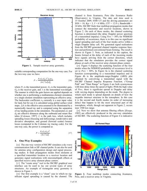
<strong>channel</strong> is from Jicamarca, Peru (the Jicamarca Radio<br />
Observatory) to Virginia. The date and time used is<br />
15 October 2009, 0300 UT and the driving parameters are<br />
SSN = 10, Kp = 3, f = 6 MHz, CIT = 12.8 s, Bandwidth =<br />
24 kHz. <strong>HiCIRF</strong> finds four multihop propagation modes that<br />
connect the transmitter and receiver locations, shown in<br />
Figure 2. On each of these modes, the <strong>channel</strong> scattering<br />
function is determined (the delay Doppler power spectrum<br />
of a transmitted impulse). Using Perc = 50% for WBMOD<br />
probability of occurrence, there is in this case no significant<br />
signal spreading and each of the four modes arrive within a<br />
single Doppler delay cell. We generated signal realizations<br />
from the <strong>HiCIRF</strong>-generated <strong>channel</strong> impulse response function<br />
and performed conventional beam forming. The result is<br />
shown in Figure 3. Note, as indicated in the caption, the<br />
beams formed at the delay of each of the incoming modes<br />
have signals arriving from the correct directions, which<br />
indicates that the <strong>simulation</strong> provides the correct signal<br />
phases at each of the receiver array element phase centers.<br />
[29] Figure 4 displays the scattering function of the four<br />
modes when the WBMOD probability of occurrence level is<br />
set to Perc = 80%. In Figure 4a is the <strong>channel</strong> scattering<br />
function (corresponding to a transmitted impulse) and in<br />
Figure 4b is the amplitude-range-Doppler (ARD) plot<br />
obtained by convolving a transmitted signal with the<br />
<strong>HiCIRF</strong> Channel Impulse Response Function. (“Group<br />
Path” and “Slant Range” in Figure 4 are both synonymous<br />
with time delay times the speed of light.) With the high value<br />
of Perc, there is significant spread in Doppler and delay<br />
with varying degree depending on the mode. The degree to<br />
which each mode is spread depends on details of how the<br />
raypaths intersect structure in the ionosphere. In this case<br />
it is the second and fourth modes (in order of increasing<br />
delay) that happen to hit the most structured part of the<br />
ionosphere, which, though not apparent in Figure 2, occurs<br />
near 1500 km range.<br />
[30] Next we show that antenna filtering effects [Knepp,<br />
1985] are effectively produced in the one-way <strong>simulation</strong><br />
of <strong>HiCIRF</strong>. The scattering function of Figure 4 is indicative<br />
P ¼ P T G T G R l 2<br />
ð4pÞ 2 : ð17Þ<br />
LdT<br />
2<br />
4. One-Way Examples<br />
[26] The one-way version of <strong>HiCIRF</strong> simulates a sky wave<br />
communication link or <strong>HF</strong> <strong>channel</strong> probe. It can also be used<br />
for antenna array configuration design and signal processing<br />
studies. It finds propagation modes from elements at<br />
a specified transmitter location to a receiver location and<br />
generates signal realizations with micromultipath effects at<br />
specified receive array element phase centers.<br />
[27] The “create array” tool in the <strong>HiCIRF</strong> graphical user<br />
interface can be used to lay out several types of array<br />
structures. An example of rectangular array geometry is<br />
shown in Figure 1.<br />
[28] Our first example is a “clean” case in which no significant<br />
signal spreading is caused by the <strong>channel</strong>. The<br />
Figure 2. Four multihop modes connecting Jicamarca,<br />
Peru, and a receiver array in Virginia.<br />
5of10