1 In this appendix I discuss the computational details of the ...
1 In this appendix I discuss the computational details of the ...
1 In this appendix I discuss the computational details of the ...

You also want an ePaper? Increase the reach of your titles
YUMPU automatically turns print PDFs into web optimized ePapers that Google loves.
APPENDIX TO "A PRACTITIONER’S GUIDE TO ESTIMATION OF RANDOM COEFFICIENTS LOGIT<br />
MODELS OF DEMAND” –<br />
ESTIMATION: THE NITTY-GRITTY<br />
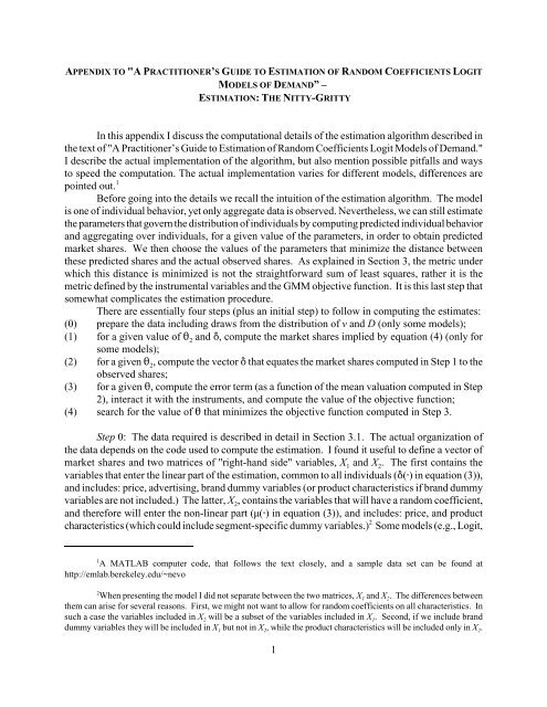
<strong>In</strong> <strong>this</strong> <strong>appendix</strong> I <strong>discuss</strong> <strong>the</strong> <strong>computational</strong> <strong>details</strong> <strong>of</strong> <strong>the</strong> estimation algorithm described in<br />
<strong>the</strong> text <strong>of</strong> "A Practitioner’s Guide to Estimation <strong>of</strong> Random Coefficients Logit Models <strong>of</strong> Demand."<br />
I describe <strong>the</strong> actual implementation <strong>of</strong> <strong>the</strong> algorithm, but also mention possible pitfalls and ways<br />
to speed <strong>the</strong> computation. The actual implementation varies for different models, differences are<br />
pointed out. 1<br />
Before going into <strong>the</strong> <strong>details</strong> we recall <strong>the</strong> intuition <strong>of</strong> <strong>the</strong> estimation algorithm. The model<br />
is one <strong>of</strong> individual behavior, yet only aggregate data is observed. Never<strong>the</strong>less, we can still estimate<br />
<strong>the</strong> parameters that govern <strong>the</strong> distribution <strong>of</strong> individuals by computing predicted individual behavior<br />
and aggregating over individuals, for a given value <strong>of</strong> <strong>the</strong> parameters, in order to obtain predicted<br />
market shares. We <strong>the</strong>n choose <strong>the</strong> values <strong>of</strong> <strong>the</strong> parameters that minimize <strong>the</strong> distance between<br />
<strong>the</strong>se predicted shares and <strong>the</strong> actual observed shares. As explained in Section 3, <strong>the</strong> metric under<br />
which <strong>this</strong> distance is minimized is not <strong>the</strong> straightforward sum <strong>of</strong> least squares, ra<strong>the</strong>r it is <strong>the</strong><br />
metric defined by <strong>the</strong> instrumental variables and <strong>the</strong> GMM objective function. It is <strong>this</strong> last step that<br />
somewhat complicates <strong>the</strong> estimation procedure.<br />
There are essentially four steps (plus an initial step) to follow in computing <strong>the</strong> estimates:<br />
(0) prepare <strong>the</strong> data including draws from <strong>the</strong> distribution <strong>of</strong> v and D (only some models);<br />
(1) for a given value <strong>of</strong> 2 2 and *, compute <strong>the</strong> market shares implied by equation (4) (only for<br />
some models);<br />
(2) for a given 2 2 , compute <strong>the</strong> vector * that equates <strong>the</strong> market shares computed in Step 1 to <strong>the</strong><br />
observed shares;<br />
(3) for a given 2, compute <strong>the</strong> error term (as a function <strong>of</strong> <strong>the</strong> mean valuation computed in Step<br />
2), interact it with <strong>the</strong> instruments, and compute <strong>the</strong> value <strong>of</strong> <strong>the</strong> objective function;<br />
(4) search for <strong>the</strong> value <strong>of</strong> 2 that minimizes <strong>the</strong> objective function computed in Step 3.<br />
Step 0: The data required is described in detail in Section 3.1. The actual organization <strong>of</strong><br />
<strong>the</strong> data depends on <strong>the</strong> code used to compute <strong>the</strong> estimation. I found it useful to define a vector <strong>of</strong><br />
market shares and two matrices <strong>of</strong> "right-hand side" variables, X 1 and X 2 . The first contains <strong>the</strong><br />
variables that enter <strong>the</strong> linear part <strong>of</strong> <strong>the</strong> estimation, common to all individuals (*(@) in equation (3)),<br />
and includes: price, advertising, brand dummy variables (or product characteristics if brand dummy<br />
variables are not included.) The latter, X 2 , contains <strong>the</strong> variables that will have a random coefficient,<br />
and <strong>the</strong>refore will enter <strong>the</strong> non-linear part (µ(@) in equation (3)), and includes: price, and product<br />
characteristics (which could include segment-specific dummy variables.) 2 Some models (e.g., Logit,<br />
1<br />
A MATLAB computer code, that follows <strong>the</strong> text closely, and a sample data set can be found at<br />
http://emlab.berekeley.edu/~nevo<br />
2<br />
When presenting <strong>the</strong> model I did not separate between <strong>the</strong> two matrices, X 1 and X 2 . The differences between<br />
<strong>the</strong>m can arise for several reasons. First, we might not want to allow for random coefficients on all characteristics. <strong>In</strong><br />
such a case <strong>the</strong> variables included in X 2 will be a subset <strong>of</strong> <strong>the</strong> variables included in X 1 . Second, if we include brand<br />
dummy variables <strong>the</strong>y will be included in X 1 but not in X 2 , while <strong>the</strong> product characteristics will be included only in X 2 .<br />
1
Nested Logit, and GEV) do not have random coefficients, <strong>the</strong> non-linear part is set to zero, and<br />
<strong>the</strong>refore only <strong>the</strong> first design matrix, X 1 , is required.<br />
Next, we sample a set <strong>of</strong> "individuals". Each "individual" consists <strong>of</strong> a K-dimensional vector<br />
<strong>of</strong> shocks that determine <strong>the</strong> individual’s taste parameters, v i<br />
'(v 1<br />
i ,...,v K<br />
i ), demographics,<br />
D i<br />
'(D i1<br />
,...,D id<br />
), and potentially a vector <strong>of</strong> shocks to <strong>the</strong> utility,<br />
i '( i0 ,..., iJ ) . Let ns be <strong>the</strong><br />
number <strong>of</strong> individuals sampled. The use <strong>of</strong> <strong>this</strong> "individual data" is explained below, in Step 1. <strong>In</strong><br />
most cases we will not need to draw<br />
i, since we can integrate <strong>the</strong> extreme value shocks analytically<br />
(see <strong>details</strong> below.) That is also <strong>the</strong> reason we do not need <strong>the</strong>se draws for <strong>the</strong> Logit, Nested Logit<br />
and GEV models.<br />
The sample <strong>of</strong> individuals can be generated in two ways: by assuming a parametric functional<br />
form, or using <strong>the</strong> empirical non-parametric distribution <strong>of</strong> real individuals. Shocks that determine<br />
<strong>the</strong> individuals taste parameters, v, are usually drawn from a multi-variate normal distribution. <strong>In</strong><br />
principle, <strong>the</strong>se could be drawn from any o<strong>the</strong>r parametric distribution. 3 The choice <strong>of</strong> <strong>the</strong><br />
distribution depends on <strong>the</strong> problem at hand and on <strong>the</strong> researcher’s beliefs. Demographics are<br />
drawn from <strong>the</strong> CPS; instead <strong>of</strong> assuming parametric forms for <strong>the</strong> distribution <strong>of</strong> demographics real<br />
individuals are sampled. This, <strong>of</strong> course, has <strong>the</strong> advantage <strong>of</strong> not depending on a somewhat<br />
arbitrary assumption <strong>of</strong> a parametric distributional form. On <strong>the</strong> o<strong>the</strong>r hand, if <strong>the</strong> parametric form<br />
was correct <strong>the</strong>n using <strong>the</strong> non-parametric approach will be less efficient. The choice <strong>of</strong> parametric<br />
versus non-parametric form should depend on <strong>the</strong> researcher’s believe on how well a parametric<br />
function can explain <strong>the</strong> distribution <strong>of</strong> demographics.<br />
As pointed out, <strong>the</strong> data consists <strong>of</strong> observations on prices and market shares <strong>of</strong> different<br />
brands in several markets. <strong>In</strong> <strong>the</strong>ory we could consider drawing different individuals for each<br />
observation, i.e., each brand in each market. However, in order for Step 2 to work we require that<br />
<strong>the</strong> predicted market shares sum up to one, which requires that we use <strong>the</strong> same draws for each<br />
market.<br />
There is a question <strong>of</strong> whe<strong>the</strong>r <strong>the</strong>se draws should vary between markets. Once again, <strong>the</strong><br />
answer depends on <strong>the</strong> specifics <strong>of</strong> <strong>the</strong> problem and <strong>the</strong> data. <strong>In</strong> general, <strong>the</strong> draws should be <strong>the</strong><br />
same whenever it is <strong>the</strong> same individuals making <strong>the</strong> decisions. For example, BLP use national<br />
market shares <strong>of</strong> different brands <strong>of</strong> cars over twenty years. They use <strong>the</strong> same draws for all<br />
markets.<br />
Finally, it is important to draw <strong>the</strong>se only once at <strong>the</strong> beginning <strong>of</strong> <strong>the</strong> computation. If <strong>the</strong><br />
draws are changed during <strong>the</strong> computation <strong>the</strong> non-linear search is unlikely to converge.<br />
Step 1: Now that we have a sample <strong>of</strong> individuals (each described by (v, D, g)), for a given<br />
value <strong>of</strong> <strong>the</strong> parameters, 2 2 , and <strong>the</strong> component common to all consumers, *, we compute <strong>the</strong><br />
predicted market shares given by <strong>the</strong> integral in equation (4). For many models (e.g., Logit, Nested<br />
Logit and PD GEV) <strong>this</strong> step can be performed analytically.<br />
For <strong>the</strong> full random coefficients model <strong>this</strong> integral has to be computed by simulation. There<br />
are several ways to do <strong>this</strong>. The first is <strong>the</strong> naive frequency estimator. We sample ns draws <strong>of</strong> <strong>the</strong><br />
vector (v, D, g), for each <strong>of</strong> <strong>the</strong>se we predict <strong>the</strong> brand purchased, and <strong>the</strong>n sum over <strong>the</strong> purchases.<br />
Formally, our estimator is given by<br />
s jt<br />
(p jt<br />
,x jt<br />
,<br />
.t ,P ns ; 2 )' 1 ns<br />
ns j 1 u ijt<br />
(D i<br />
,v i<br />
,<br />
i )$u ilt (D i ,v i , i ) æl'0,1,...,J ,<br />
i'1<br />
3<br />
For example, Berry, Carnall and Spiller (1996) use a two point discrete distribution.<br />
2
where 1{C}'1 if <strong>the</strong> C is true, and 0 o<strong>the</strong>rwise. This is repeated for every brand in every market.<br />
Although <strong>this</strong> approach is very intuitive it is lacking in three dimensions. First, it requires<br />
a large number <strong>of</strong> draws, ns, at least <strong>the</strong> number <strong>of</strong> products, and usually much more than that.<br />
O<strong>the</strong>rwise, <strong>the</strong> predicted market shares for some <strong>of</strong> <strong>the</strong> products will be zero. The smaller <strong>the</strong><br />
observed shares <strong>the</strong> larger <strong>the</strong> problem. Second, in <strong>this</strong> approach <strong>the</strong>re are three simulation processes<br />
that induce variance in <strong>the</strong> estimated parameters, <strong>the</strong> sampling processes <strong>of</strong> <strong>the</strong> v’s, <strong>the</strong> D’s, and <strong>the</strong><br />
g’s. While in <strong>the</strong> approach suggested below <strong>the</strong> simulation error due to <strong>the</strong> sampling process <strong>of</strong> <strong>the</strong><br />
g’s is eliminated. Finally, <strong>this</strong> approach renders a non smooth objective function, and <strong>the</strong>refore does<br />
not allow us to use gradient methods to minimize <strong>the</strong> objective function (see Step 4.)<br />
A second approach to computing <strong>the</strong> predicted market shares, which does not suffer from <strong>the</strong><br />
above problems, is <strong>the</strong> smooth simulator. Here we use <strong>the</strong> extreme value distribution, P ( ( ),to<br />
integrate <strong>the</strong> g’s analytically. Formally, <strong>the</strong> predicted market shares, given by equation (4), are<br />
approximated by<br />
s jt<br />
(p .t<br />
,x .t<br />
,<br />
.t ,P ns ; 2 )' 1 ns<br />
ns j s jti<br />
'<br />
(A-1)<br />
ns<br />
1<br />
ns j i'1<br />
K<br />
exp jt<br />
% j k'1 x k<br />
jt ( k v k<br />
i<br />
% k1<br />
D i1<br />
%...% kd<br />
D id<br />
)<br />
J<br />
1% j m'1 exp mt % j K k'1 x k mt ( k v k<br />
i<br />
% k1<br />
D i1<br />
%...% kd<br />
D id<br />
)<br />
where (v 1<br />
i ,...,v K<br />
i ) and (D i1<br />
,...D id<br />
), i'1,...,ns, are <strong>the</strong> draws from step 0, while x k<br />
jt , k'1,...,K , are<br />
<strong>the</strong> variables included in X 2 .<br />
Note, that we no longer require a large number <strong>of</strong> draws to predict non-zero market shares.<br />
Actually, one draw <strong>of</strong> <strong>the</strong> pair (v, D) will suffice (although <strong>this</strong> is by no means <strong>the</strong> recommended<br />
number.) Also, since <strong>the</strong> g’s are integrated analytically <strong>the</strong> variance due to <strong>the</strong> simulation process<br />
is limited only to <strong>the</strong> simulation <strong>of</strong> v and D. Finally, unlike before <strong>the</strong> predicted market shares are<br />
smooth functions <strong>of</strong> <strong>the</strong> parameters, and <strong>the</strong>refore a gradient method can be used to minimize <strong>the</strong><br />
objective function.<br />
<strong>In</strong> some applications efficiency <strong>of</strong> <strong>the</strong> estimator will be very important and <strong>the</strong>refore one<br />
would like to reduce <strong>the</strong> variance due to <strong>the</strong> simulation error. <strong>In</strong> principle, <strong>this</strong> can be achieved by<br />
increasing <strong>the</strong> number <strong>of</strong> draws, ns. A <strong>computational</strong> more efficient way <strong>of</strong> reducing <strong>the</strong> simulation<br />
error is to use various sampling methods, for example, importance sampling or Halton sequences.<br />
A full <strong>discuss</strong>ion <strong>of</strong> <strong>the</strong>se methods is beyond <strong>the</strong> scope <strong>of</strong> <strong>this</strong> paper (see BLP for use <strong>of</strong> importance<br />
sampling or Train, 1999, for use <strong>of</strong> Halton sequences.)<br />
Step 2: As previously pointed out, we choose our estimates by minimizing <strong>the</strong> distance <strong>of</strong><br />
<strong>the</strong> predicted market shares to <strong>the</strong> observed market shares. For <strong>the</strong> reasons given in Section 3 we<br />
will not define <strong>the</strong> distance as <strong>the</strong> sum <strong>of</strong> squares, ra<strong>the</strong>r we obtain an expression that is linear in <strong>the</strong><br />
structural error term and interact it with instruments to form a GMM objective function. This step<br />
is required in order to obtain <strong>this</strong> structural error term.<br />
We want to compute <strong>the</strong> J×T-dimensional vector <strong>of</strong> mean valuations, * jt , that equates <strong>the</strong><br />
market shares computed in Step 1 to <strong>the</strong> observed shares. This amounts to solving separately for<br />
each market <strong>the</strong> system <strong>of</strong> equations 4<br />
i'1<br />
,<br />
4<br />
Berry (1994) proves existence and uniqueness <strong>of</strong> <strong>the</strong> vector .<br />
3
(A-2)<br />
s .t<br />
;<br />
2 'S .t<br />
t'1,...,T,<br />
where s(@) are <strong>the</strong> predicted market shares computed in Step 1 and S are <strong>the</strong> observed market shares.<br />
This system is solved market by market.<br />
For <strong>the</strong> Logit model <strong>this</strong> inversion can be computed analytically by<br />
jt 'ln(S jt )&ln(S 0t ) ,<br />
where S 0t is <strong>the</strong> market share <strong>of</strong> <strong>the</strong> outside good, computed by subtracting <strong>the</strong> sum <strong>of</strong> observed<br />
market shares <strong>of</strong> all <strong>the</strong> inside goods from 1. Note, it is <strong>the</strong> observed market shares that enter <strong>this</strong><br />
equation, and <strong>the</strong>refore we do not require Step 1 for <strong>the</strong> Logit model. This inversion can also be<br />
computed analytically in <strong>the</strong> Nested Logit model (see Berry, 1994) and <strong>the</strong> PD GEV model<br />
(Bresnahan, Stern and Trajtenberg, 1997.)<br />
For <strong>the</strong> full model <strong>the</strong> system <strong>of</strong> equations (A-2) is non-linear and is solved numerically. It<br />
can be solved by using <strong>the</strong> contraction mapping suggested by BLP (see <strong>the</strong>re for pro<strong>of</strong> <strong>of</strong><br />
convergence), which amounts to computing <strong>the</strong> series<br />
(A-3)<br />
h%1<br />
.t ' ḥ t %ln(S .t )&ln s(p .t ,x .t , h<br />
.t ,P ns ; 2<br />
), t'1,...,T, h'0,...,H,<br />
where s(@) are <strong>the</strong> predicted market shares computed in Step 1, H is <strong>the</strong> smallest integer such that<br />
2 Ḥ t & H&1<br />
H<br />
.t 2is smaller than some tolerance level, and .t is <strong>the</strong> approximation to<br />
.t.<br />
A few practical points. First, convergence can be reached faster by choosing a good starting<br />
0<br />
H<br />
value, .t. I use <strong>the</strong> value, .t , computed from <strong>the</strong> last iteration <strong>of</strong> <strong>the</strong> objective function, with <strong>the</strong><br />
first iteration using <strong>the</strong> values that solve <strong>the</strong> Logit model, i.e,<br />
0<br />
jt 'log(S jt )&log(S 0t ).<br />
Better approximations can be derived (for example, using <strong>the</strong> derivative <strong>of</strong> *(@) computed below, <strong>the</strong><br />
first term <strong>of</strong> a Taylor approximation can be computed.) However, I found that computing better<br />
approximations usually took longer than <strong>the</strong> time saved.<br />
Second, <strong>the</strong> fur<strong>the</strong>r away from <strong>the</strong> true value <strong>of</strong> <strong>the</strong> parameters we are, <strong>the</strong> harder it is to solve<br />
<strong>the</strong> system <strong>of</strong> equations (A-2). Therefore, I found it helpful to change <strong>the</strong> tolerance level as <strong>the</strong><br />
number <strong>of</strong> iterations in <strong>the</strong> process defined by equation (A-3) goes up. For example, for <strong>the</strong> first 100<br />
iterations, <strong>of</strong> <strong>the</strong> process defined in equation (A-3), <strong>the</strong> tolerance level is set to 10E-8, while after<br />
that every additional 50 iterations <strong>the</strong> tolerance level increases by an order <strong>of</strong> ten. If <strong>the</strong> change in<br />
<strong>the</strong> value <strong>of</strong> <strong>the</strong> parameters was low (say less than 0.01) <strong>the</strong> tolerance level was kept at its initial<br />
value. This promises that near <strong>the</strong> solution <strong>the</strong> inversion is computed very accurately, while <strong>the</strong><br />
algorithm does not waste time far away from <strong>the</strong> solution, where <strong>the</strong> number <strong>of</strong> iterations required<br />
to achieve accurate convergence <strong>of</strong> <strong>the</strong> process defined in equation (A-3) is high.<br />
Third, a trivial point but one that can save several days <strong>of</strong> work: <strong>the</strong> order <strong>of</strong> <strong>the</strong> terms in<br />
equation (A-3) matters, o<strong>the</strong>rwise <strong>the</strong> contraction mapping does not work (ra<strong>the</strong>r than getting closer<br />
to <strong>the</strong> solution <strong>the</strong> series will get fur<strong>the</strong>r away).<br />
Finally, since computing exponents and logarithms is <strong>computational</strong>ly demanding <strong>the</strong><br />
contraction mapping, defined by equation (A-3), can be solved by solving for <strong>the</strong> exponent <strong>of</strong> <strong>the</strong><br />
vector *. I.e., define w jt<br />
'exp( jt<br />
) and solve<br />
w h%1<br />
jt<br />
'w h<br />
jt<br />
s jt<br />
(p .t<br />
,x .t<br />
,<br />
S jt<br />
, t'1,...,T, h'0,...,H,<br />
h<br />
.t ,P ns ; 2 )<br />
where <strong>the</strong> starting value is w 0<br />
.t 'exp( 0 .t ) H<br />
and .t 'log(w H<br />
.t ) is <strong>the</strong> same as <strong>the</strong> solution to <strong>the</strong><br />
4
contraction mapping, defined by equation (A-3). This greatly reduces <strong>the</strong> number <strong>of</strong> exponents and<br />
logarithms computed.<br />
Step 3: Finally we can compute <strong>the</strong> error term. For all <strong>the</strong> models previously described it is<br />
defined by<br />
' &X 1 1<br />
,<br />
where * is <strong>the</strong> J×T-dimensional vector computed in Step 2, X 1 is <strong>the</strong> design matrix defined in Step<br />
0, and 2 1 is <strong>the</strong> vector <strong>of</strong> linear parameters. This is interacted in a straightforward way with <strong>the</strong><br />
instrument matrix to form <strong>the</strong> moment conditions, which are used to compute <strong>the</strong> objective function<br />
( ) ) Z &1 Z ) ( ),<br />
where M is a consistent estimate <strong>of</strong> E[Z ) ) Z] .<br />
Like many GMM estimation problems, <strong>the</strong> computation <strong>of</strong> <strong>the</strong> objective function requires<br />
knowledge <strong>of</strong> <strong>the</strong> weight matrix, which in general requires knowledge <strong>of</strong> <strong>the</strong> true value <strong>of</strong> <strong>the</strong><br />
parameters (or a consistent estimate <strong>the</strong>re<strong>of</strong>.) There are several solutions to <strong>this</strong> problem. First,<br />
assume homoscedastic errors and <strong>the</strong>refore <strong>the</strong> optimal weight matrix is proportional to Z ) Z, thus,<br />
<strong>the</strong> need to know <strong>the</strong> true parameter values is eliminated. Second, we can compute an estimate <strong>of</strong><br />
2, say ˆ , using 'Z ) Z, and <strong>the</strong>n use <strong>this</strong> estimate to compute a new weight matrix<br />
E[Z ) (ˆ) (ˆ) ) Z], which in turn is used to compute a new estimate <strong>of</strong> 2.<br />
&1<br />
An additional option is to continue iterating between <strong>the</strong> estimates <strong>of</strong> 2 and until<br />
convergence. Hansen, Heaton and Yaron (1996) examine <strong>this</strong> option and also examine <strong>the</strong> estimate<br />
based on simultaneously minimizing <strong>the</strong> average moments and <strong>the</strong> weight matrix. Although <strong>the</strong>se<br />
approaches has some appeal, it is not clear in what sense <strong>the</strong>y are optimal, or which is better. Both<br />
<strong>the</strong>se approaches, as well as <strong>the</strong> previous one, are first-order asymptotically equivalent. As shown<br />
by Hansen, Heaton and Yaron (1996), for linear GMM problems, nei<strong>the</strong>r method dominates in finite<br />
samples. Therefore, I see no justification to use continuous updating in non-linear GMM problems,<br />
like <strong>the</strong> one here, where <strong>the</strong> <strong>computational</strong> costs are large.<br />
Step 4: Search for <strong>the</strong> value <strong>of</strong> 2 that minimizes <strong>the</strong> objective function. For <strong>the</strong> Logit model<br />
<strong>this</strong> can be done analytically (it is a linear GMM problem.) For <strong>the</strong> full model we need to perform<br />
a non-linear search over 2. The time required for <strong>this</strong> search can be reduced by using <strong>the</strong> first order<br />
conditions, with respect to 2 1 , to express 2 1 as a function <strong>of</strong> 2 2 , i.e.,<br />
ˆ1'(X<br />
)<br />
1 Z &1 Z ) X 1<br />
) &1 X ) 1 Z &1 Z )<br />
(ˆ2),<br />
where X 1 is <strong>the</strong> design matrix and Z is <strong>the</strong> instrument matrix. Now, <strong>the</strong> non-linear search can be<br />
limited to 2 2 .<br />
One <strong>of</strong> two search methods is usually used, ei<strong>the</strong>r <strong>the</strong> Nelder-Mead (1965) non-derivative<br />
"simplex" search method, or a quasi-Newton method with an analytic gradient (see Press et al., 1994,<br />
and references <strong>the</strong>rein.) The first is more robust but is much slower to converge, while <strong>the</strong> latter is<br />
two orders <strong>of</strong> magnitude faster, yet is sensitive to starting values. If <strong>the</strong> initial values are extremely<br />
poor <strong>the</strong> algorithm would reach regions where <strong>the</strong> objective is not defined. This is especially true<br />
if <strong>the</strong> variables are scaled differently, i.e., one characteristic will range from 1 to 5 while ano<strong>the</strong>r<br />
from 0 to 250.<br />
A useful trick is to set <strong>the</strong> value <strong>of</strong> <strong>the</strong> objective function to a high number (say 10E+10) if<br />
one <strong>of</strong> its components is not defined. This allows <strong>the</strong> algorithm to deal with situations in which <strong>the</strong><br />
objective function is not defined. Poor starting values, different scaling <strong>of</strong> <strong>the</strong> variables, and <strong>the</strong><br />
5
non-linear objective would cause <strong>this</strong> to happen. This usually happens in <strong>the</strong> first few iterations,<br />
especially if <strong>the</strong> parameters are not properly scaled. An alternative way <strong>of</strong> dealing with <strong>this</strong> problem<br />
is to decrease <strong>the</strong> initial step size (i.e., <strong>the</strong> step taken in <strong>the</strong> direction determined by <strong>the</strong> negative <strong>of</strong><br />
<strong>the</strong> gradient.) The recommended practice is to start with <strong>the</strong> non-derivative method and switch to <strong>the</strong><br />
gradient method once <strong>the</strong> objective has been lowered to reasonable levels.<br />
The main increase in speed using <strong>the</strong> gradient method comes from using an analytic gradient<br />
function. Using a gradient computed from finite differences results in relatively less increase in<br />
speed, while maintaining all <strong>the</strong> problems <strong>of</strong> <strong>the</strong> gradient method. <strong>In</strong> order for <strong>the</strong> gradient to be<br />
well defined everywhere, <strong>the</strong> simulated market shares have to be smooth functions <strong>of</strong> <strong>the</strong> parameters.<br />
The smooth simulator <strong>discuss</strong>ed above has <strong>this</strong> property, while <strong>the</strong> naive frequency simulator does<br />
not.<br />
<strong>In</strong> order to compute <strong>the</strong> gradient <strong>of</strong> <strong>the</strong> objective function, <strong>the</strong> derivative <strong>of</strong> <strong>the</strong> function<br />
computed in Step 2 has to be computed. The mean valuations <strong>of</strong> <strong>the</strong> J brands in each market are<br />
implicitly defined by <strong>the</strong> system <strong>of</strong> J equations given in (A-2). By <strong>the</strong> Implicit Function Theorem<br />
(see, for example, Simon and Blume, 1994, Theorem 15.7 pg 355) <strong>the</strong> derivatives <strong>of</strong> <strong>the</strong> mean value<br />
with respect to <strong>the</strong> parameters are<br />
(A-4)<br />
D .t<br />
'<br />
M 1t<br />
M 21<br />
ã M 1t<br />
M 2L<br />
! " !<br />
M Jt<br />
M 21<br />
ã M Jt<br />
M 2L<br />
'&<br />
Ms 1t<br />
M 1t<br />
ã Ms 1t<br />
M Jt<br />
! " !<br />
Ms Jt<br />
M 1t<br />
ã Ms Jt<br />
M Jt<br />
&1<br />
Ms 1t<br />
M 21<br />
ã Ms 1t<br />
M 2L<br />
! " ! ,<br />
Ms Jt<br />
ã Ms Jt<br />
M 21<br />
M 2L<br />
where<br />
2i , i'1,...,L denotes <strong>the</strong> i’s element <strong>of</strong> <strong>the</strong> vector 2 2 , which contains <strong>the</strong> non-linear<br />
parameters <strong>of</strong> <strong>the</strong> model. The share function defined by <strong>the</strong> smooth simulator is given in equation<br />
(A-1). Therefore, <strong>the</strong> derivatives are<br />
Ms jt<br />
' 1 ns<br />
Ms<br />
ns j jti<br />
' 1 ns<br />
M jt<br />
ns j s jti<br />
(1&s jti<br />
)<br />
M jt<br />
i'1<br />
i'1<br />
Ms jt<br />
M mt<br />
' 1 ns j ns<br />
i'1<br />
Ms jti<br />
M mt<br />
' & 1 ns j ns<br />
i'1<br />
s jti<br />
s mti<br />
Ms jt<br />
M k<br />
' 1 ns j ns<br />
i'1<br />
Ms jti<br />
M k<br />
' 1 ns j ns<br />
i'1<br />
s ji<br />
x k<br />
jt v k<br />
i & j<br />
J<br />
m'1<br />
x k mt v k<br />
i s mti<br />
' 1 ns j ns<br />
i'1<br />
v k<br />
i s jti<br />
x k<br />
J<br />
jt & j x k mt s mti<br />
m'1<br />
Ms jt<br />
M kd<br />
' 1 ns j ns<br />
i'1<br />
Ms jti<br />
M kd<br />
' 1 ns j ns<br />
i'1<br />
s jti<br />
J<br />
jt D id & j x k mt D id s mti<br />
' 1 ns<br />
ns j<br />
x k<br />
m'1<br />
i'1<br />
D id<br />
s jti<br />
x k<br />
J<br />
jt & j x k mt s mti<br />
Substituting <strong>this</strong> back into equation (A-4), we obtain <strong>the</strong> derivative <strong>of</strong> <strong>the</strong> function computed in Step<br />
2.<br />
The gradient <strong>of</strong> <strong>the</strong> objective function is<br />
2(D ) (Z( &1 (Z ) ( .<br />
m'1<br />
6
Once <strong>this</strong> is programed it is easy to check by comparing <strong>the</strong> results to <strong>the</strong> gradient computed using<br />
finite differences. If such a comparison is made, <strong>the</strong>n <strong>the</strong> tolerance levels in Step 2 have to be set low<br />
(10E-8), and not allowed to vary (see <strong>discuss</strong>ion above.)<br />
ADDITIONAL REFERENCES (not referenced in <strong>the</strong> main text).<br />
Hansen, L.P., J. Heaton, and A. Yaron (1996), “Finite Sample Properties <strong>of</strong> Some Alternative GMM<br />
Estimators,” Journal <strong>of</strong> Business and Economic Statistics, 14(3), 262-80.<br />
Nelder, J.A., and R. Mead (1965), “A Simplex Method for Function Minimization,” Computer Journal, Vol.<br />
7, 308-313.<br />
Press, W.H., S.A. Teukolsky, W.T. Vetterling, and B.P. Flannery (1994), Numerical Recipes in C,<br />
Cambridge University Press.<br />
Simon, C.P. , and L. Blume (1994), Ma<strong>the</strong>matics for Economists, New York: W. W. Norton & Company.<br />
Train, K. (1999), “Halton Sequences for Mixed Logit,” University <strong>of</strong> California at Berkeley, mimeo.<br />
7