Real-Time GPU Silhouette Refinement using adaptively blended ...
Real-Time GPU Silhouette Refinement using adaptively blended ...
Real-Time GPU Silhouette Refinement using adaptively blended ...

You also want an ePaper? Increase the reach of your titles
YUMPU automatically turns print PDFs into web optimized ePapers that Google loves.
and shading normals of each triangle in Ω to construct a<br />
corresponding cubic Bézier patch. The end result of our<br />
construction is a set of triangular patches that constitutes<br />
a piecewise smooth surface. Our construction is a variant<br />
of the one in [7], see also [22].<br />
For each edge e ij in Ω, we determine a cubic Bézier<br />
curve based on the edge endpoints v i , v j and their associated<br />
shading normals:<br />
C ij (t) = v i B 3 0(t) + c ij B 3 1(t) + c ji B 3 2(t) + v j B 3 3(t),<br />
where Bi 3(t) = ( 3<br />
i)<br />
t i (1 − t) 3−i are the Bernstein polynomials,<br />
see e.g. [8]. The inner control point c ij is determined<br />
as follows. Let T s and T t be the two triangles adjacent<br />
to e ij and let n si and n ti be the shading normals at v i<br />
belonging to triangle T s and T t respectively. If n si = n ti ,<br />
we say that v i is a smooth edge end and we determine its<br />
inner control point as c ij = 2vi+vj<br />
3<br />
− (vj−vi)·nsi<br />
3<br />
n si . On<br />
the other hand, if n si ≠ n ti , we say that v i is a sharp<br />
edge end and let c ij = v i + (vj−vi)·tij<br />
3<br />
t ij , where t ij is<br />
the normalized cross product of the shading normals. We<br />
refer to [7] for the rationale behind this construction.<br />
Next, we use the control points of the three edge curves<br />
belonging to a triangle [v i , v j , v k ] to define nine of the<br />
ten control points of a cubic triangular Bézier patch of the<br />
form<br />
F =<br />
∑<br />
b lmn Blmn. 3 (3)<br />
l+m+n=3<br />
Here B 3 lmn = 6<br />
l!m!n! ul v m w n are the Bernstein-Bézier<br />
polynomials and u, v, w are barycentric coordinates, see<br />
e.g. [8]. We determine the coefficients such that b 300 =<br />
v i , b 210 = c ij , b 120 = c ji and so forth. In [22] and [7]<br />
the center control point b 111 was determined as<br />
b 111 = 3<br />
12 (c ij + c ji + c jk + c kj + c ki + c ik ) (4)<br />
− 1 6 (v i + v j + v k ) .<br />
We propose instead to optionally use the average of the<br />
inner control points of the three edge curves,<br />
b 111 = 1 6 (c ij + c ji + c jk + c kj + c ki + c ik ) . (5)<br />
This choice allows for a significantly more efficient implementation<br />
at the cost of a slightly “flatter” patch, see<br />
Section 6.4 and Figure 4. This example is typical in that<br />
the patches resulting from the two formulations are visually<br />
almost indistinguishable.<br />
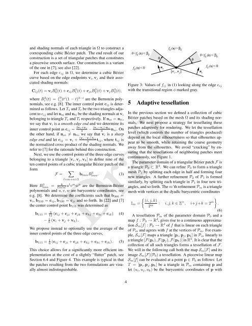
0<br />
β<br />
ij<br />
v i<br />
v j<br />
ij<br />
[ , ]<br />
φ<br />
0