Real-Time GPU Silhouette Refinement using adaptively blended ...
Real-Time GPU Silhouette Refinement using adaptively blended ...
Real-Time GPU Silhouette Refinement using adaptively blended ...

You also want an ePaper? Increase the reach of your titles
YUMPU automatically turns print PDFs into web optimized ePapers that Google loves.
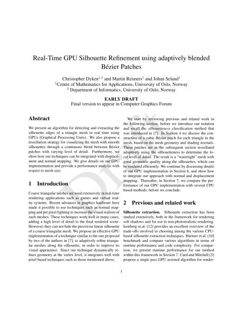
<strong>Real</strong>-<strong>Time</strong> <strong>GPU</strong> <strong>Silhouette</strong> <strong>Refinement</strong> <strong>using</strong> <strong>adaptively</strong> <strong>blended</strong><br />
Bézier Patches<br />
Christopher Dyken 1,2 and Martin Reimers 1 and Johan Seland 1<br />
1 Centre of Mathematics for Applications, University of Oslo, Norway<br />
2 Department of Informatics, University of Oslo, Norway<br />
Abstract<br />
EARLY DRAFT<br />
Final version to appear in Computer Graphics Forum<br />
We present an algorithm for detecting and extracting the<br />
silhouette edges of a triangle mesh in real time <strong>using</strong><br />
<strong>GPU</strong>s (Graphical Processing Units). We also propose a<br />
tessellation strategy for visualizing the mesh with smooth<br />
silhouettes through a continuous blend between Bézier<br />
patches with varying level of detail. Furthermore, we<br />
show how our techniques can be integrated with displacement<br />
and normal mapping. We give details on our <strong>GPU</strong><br />
implementation and provide a performance analysis with<br />
respect to mesh size.<br />
1 Introduction<br />
Coarse triangular meshes are used extensively in real-time<br />
rendering applications such as games and virtual reality<br />
systems. Recent advances in graphics hardware have<br />
made it possible to use techniques such as normal mapping<br />
and per pixel lighting to increase the visual realism of<br />
such meshes. These techniques work well in many cases,<br />
adding a high level of detail to the final rendered scene.<br />
However, they can not hide the piecewise linear silhouette<br />
of a coarse triangular mesh. We propose an effective <strong>GPU</strong><br />
implementation of a technique similar to the one proposed<br />
by two of the authors in [7], to <strong>adaptively</strong> refine triangular<br />
meshes along the silhouette, in order to improve its<br />
visual appearance. Since our technique dynamically refines<br />
geometry at the vertex level, it integrates well with<br />
pixel based techniques such as those mentioned above.<br />
We start by reviewing previous and related work in<br />
the following section, before we introduce our notation<br />
and recall the silhouetteness classification method that<br />
was introduced in [7]. In Section 4 we discuss the construction<br />
of a cubic Bézier patch for each triangle in the<br />
mesh, based on the mesh geometry and shading normals.<br />
These patches are in the subsequent section tessellated<br />
<strong>adaptively</strong> <strong>using</strong> the silhouetteness to determine the local<br />
level of detail. The result is a “watertight” mesh with<br />
good geometric quality along the silhouettes, which can<br />
be rendered efficiently. We continue by discussing details<br />
of our <strong>GPU</strong> implementation in Section 6, and show how<br />
to integrate our approach with normal and displacement<br />
mapping. Thereafter, in Section 7, we compare the performance<br />
of our <strong>GPU</strong> implementation with several CPU<br />
based methods, before we conclude.<br />
Draft<br />
Draft<br />
2 Previous and related work<br />
<strong>Silhouette</strong> extraction. <strong>Silhouette</strong> extraction has been<br />
studied extensively, both in the framework for rendering<br />
soft shadows and for use in non-photorealistic-rendering.<br />
Isenberg et.al. [12] provides an excellent overview of the<br />
trade-offs involved in choosing among the various CPUbased<br />
silhouette extraction techniques. Hartner et.al. [10]<br />
benchmark and compare various algorithms in terms of<br />
runtime performance and code complexity. For comparison,<br />
we present runtime performance for our method<br />
within this framework in Section 7. Card and Mitchell [5]<br />
propose a single pass <strong>GPU</strong> assisted algorithm for render-<br />
1
Figure 1: A dynamic refinement (left) of a coarse geometry (center). Cracking between patches of different refinement<br />
levels (top right) is eliminated <strong>using</strong> the technique described in Section 5 (bottom right).<br />
ing silhouette edges, by degenerating all non silhouette<br />
edges in a vertex shader.<br />
Curved geometry. Curved point-normal triangle<br />
patches (PN-triangles), introduced by Vlachos et.al. [22],<br />
do not need triangle connectivity between patches, and<br />
are therefore well suited for tessellation in hardware.<br />
An extension allowing for finer control of the resulting<br />
patches was presented by Boubekeur et.al. [2] and dubbed<br />
scalar tagged PN-triangles. A similar approach is taken<br />
by van Overveld and Wyvill [21], where subdivision was<br />
used instead of Bézier patches. Alliez et.al. describe a<br />
local refinement technique for subdivision surfaces [1].<br />
Adaptivity and multi resolution meshes. Multi resolution<br />
methods for adaptive rendering have a long history,<br />
a survey is given by Luebke et.al. [14]. Some examples<br />
are progressive meshes, where refinement is done<br />
by repeated triangle splitting and deletion by Hoppe [11],<br />
or triangle subdivision as demonstrated by Pulli and Segal<br />
[16] and Kobbelt [13].<br />
<strong>GPU</strong> techniques. Global subdivision <strong>using</strong> a <strong>GPU</strong> kernel<br />
is described by Shiue et.al. [19] and an adaptive subdivision<br />
technique <strong>using</strong> <strong>GPU</strong>s is given by Bunnel [4].<br />
A <strong>GPU</strong> friendly technique for global mesh refinement on<br />
<strong>GPU</strong>s was presented by Boubekeur and Schlick [3], <strong>using</strong><br />
pre-tessellated triangle strips stored on the <strong>GPU</strong>. Our rendering<br />
method is similar, but we extend their method by<br />
adding adaptivity to the rendered mesh.<br />
A recent trend is to utilize the performance of <strong>GPU</strong>s<br />
for non-rendering computations, often called GP<strong>GPU</strong><br />
(General-Purpose Computing on <strong>GPU</strong>s). We employ such<br />
techniques extensively in our algorithm, but forward the<br />
description of GP<strong>GPU</strong> programming to the introduction<br />
Draft<br />
Draft<br />
by Harris [9]. An overview of various applications in<br />
which GP<strong>GPU</strong> techniques have successfully been used<br />
is presented in Owens et.al. [15]. For information about<br />
OpenGL and the OpenGL Shading Language see the reference<br />
material by Shreiner et.al. [20] and Rost [17].<br />
3 <strong>Silhouette</strong>s of triangle meshes<br />
We consider a closed triangle mesh Ω with consistently<br />
oriented triangles T 1 , . . . , T N and vertices v 1 , . . . , v n in<br />
R 3 . The extension to meshes with boundaries is straightforward<br />
and is omitted for brevity. An edge of Ω is<br />
defined as e ij = [v i , v j ] where [·] denotes the con-<br />
2
c jk<br />
c ij<br />
c ji<br />
c kj<br />
S 1 [F]<br />
n j<br />
v j<br />
v j<br />
v i<br />
n i v i<br />
v k<br />
n<br />
v k<br />
k<br />
c ik<br />
F<br />
c ki<br />
S 3 [F]<br />
Draft<br />
Draft<br />
S 2 [F]<br />
Figure 2: From left to right: A triangle [v i , v j , v k ] and the associated shading normals n i , n j , and n k is used to define<br />
three cubic Bézier curves and a corresponding cubic triangular Bézier patch F. The sampling operator S i yields<br />
tessellations of the patch at refinement level i.<br />
vex hull of a set. The triangle normal n t of a triangle<br />
T t = [v i , v j , v k ] is defined as the normalization of the<br />
vector (v j − v i ) × (v k − v i ). Since our interest is in<br />
rendering Ω, we also assume that we are given shading<br />
normals, n ti , n tj , n tk associated with the vertices of T t .<br />
The viewpoint x ∈ R 3 is the position of the observer and<br />
for a point v on Ω, the view direction vector is v − x. If<br />
n is the surface normal in v, we say that T is front facing<br />
in v if (v − x) · n ≤ 0, otherwise it is back facing.<br />
The silhouette of a triangle mesh is the set of edges<br />
where one of the adjacent triangles is front facing while<br />
the other is back facing. Let v ij be the midpoint of an<br />
edge e ij shared by two triangles T s and T t in Ω. Defining<br />
f ij : R 3 → R by<br />
( ) ( )<br />
vij − x<br />
f ij (x) =<br />
‖ v ij − x ‖ · n vij − x<br />
s<br />
‖ v ij − x ‖ · n t ,<br />
(1)<br />
we see that e ij is a silhouette edge when observed from x<br />
in the case f ij (x) ≤ 0.<br />
Our objective is to render Ω so that it appears to have<br />
smooth silhouettes, by <strong>adaptively</strong> refining the mesh along<br />
the silhouettes. Since the resulting silhouette curves in<br />
general do not lie in Ω, and since silhouette membership<br />
for edges is a binary function of the viewpoint, a<br />
naive implementation leads to transitional artifacts: The<br />
rendered geometry depends discontinuously on the viewpoint.<br />
In [7], a continuous silhouette test was proposed<br />
to avoid such artifacts. The silhouetteness of e ij as seen<br />
from x ∈ R 3 was defined as<br />
⎧<br />
⎪⎨ 1 if f ij (x) ≤ 0;<br />
α ij (x) = 1 − fij(x)<br />
β ij<br />
if 0 < f ij (x) ≤ β ij ; (2)<br />
⎪⎩<br />
0 if f ij (x) > β ij ,<br />
where β ij > 0 is a constant. We let β ij depend on the<br />
local geometry, so that the transitional region define a<br />
“wedge” with angle φ with the adjacent triangles, see Figure<br />
3. This amounts to setting β ij = sin φ cos φ sin θ +<br />
sin 2 φ cos θ, where θ is the angle between the normals of<br />
the two adjacent triangles. We also found that the heuristic<br />
choice of β ij = 1 4<br />
works well in practice, but this<br />
choice gives unnecessary refinement over flatter areas.<br />
The classification (2) extends the standard binary classification<br />
by adding a transitional region. A silhouetteness<br />
α ij ∈ (0, 1) implies that e ij is nearly a silhouette edge.<br />
We use silhouetteness to control the view dependent interpolation<br />
between silhouette geometry and non-silhouette<br />
geometry.<br />
4 Curved geometry<br />
We assume that the mesh Ω and its shading normals are<br />
sampled from a piecewise smooth surface (it can however<br />
have sharp edges) at a sampling rate that yields nonsmooth<br />
silhouettes. In this section we use the vertices<br />
3
and shading normals of each triangle in Ω to construct a<br />
corresponding cubic Bézier patch. The end result of our<br />
construction is a set of triangular patches that constitutes<br />
a piecewise smooth surface. Our construction is a variant<br />
of the one in [7], see also [22].<br />
For each edge e ij in Ω, we determine a cubic Bézier<br />
curve based on the edge endpoints v i , v j and their associated<br />
shading normals:<br />
C ij (t) = v i B 3 0(t) + c ij B 3 1(t) + c ji B 3 2(t) + v j B 3 3(t),<br />
where Bi 3(t) = ( 3<br />
i)<br />
t i (1 − t) 3−i are the Bernstein polynomials,<br />
see e.g. [8]. The inner control point c ij is determined<br />
as follows. Let T s and T t be the two triangles adjacent<br />
to e ij and let n si and n ti be the shading normals at v i<br />
belonging to triangle T s and T t respectively. If n si = n ti ,<br />
we say that v i is a smooth edge end and we determine its<br />
inner control point as c ij = 2vi+vj<br />
3<br />
− (vj−vi)·nsi<br />
3<br />
n si . On<br />
the other hand, if n si ≠ n ti , we say that v i is a sharp<br />
edge end and let c ij = v i + (vj−vi)·tij<br />
3<br />
t ij , where t ij is<br />
the normalized cross product of the shading normals. We<br />
refer to [7] for the rationale behind this construction.<br />
Next, we use the control points of the three edge curves<br />
belonging to a triangle [v i , v j , v k ] to define nine of the<br />
ten control points of a cubic triangular Bézier patch of the<br />
form<br />
F =<br />
∑<br />
b lmn Blmn. 3 (3)<br />
l+m+n=3<br />
Here B 3 lmn = 6<br />
l!m!n! ul v m w n are the Bernstein-Bézier<br />
polynomials and u, v, w are barycentric coordinates, see<br />
e.g. [8]. We determine the coefficients such that b 300 =<br />
v i , b 210 = c ij , b 120 = c ji and so forth. In [22] and [7]<br />
the center control point b 111 was determined as<br />
b 111 = 3<br />
12 (c ij + c ji + c jk + c kj + c ki + c ik ) (4)<br />
− 1 6 (v i + v j + v k ) .<br />
We propose instead to optionally use the average of the<br />
inner control points of the three edge curves,<br />
b 111 = 1 6 (c ij + c ji + c jk + c kj + c ki + c ik ) . (5)<br />
This choice allows for a significantly more efficient implementation<br />
at the cost of a slightly “flatter” patch, see<br />
Section 6.4 and Figure 4. This example is typical in that<br />
the patches resulting from the two formulations are visually<br />
almost indistinguishable.<br />
0<br />
β<br />
ij<br />
v i<br />
v j<br />
ij<br />
[ , ]<br />
φ<br />
0
espect to T . Then p = u i p i + u j p j + u k p k and<br />
S m [f](p) = u i f(p i ) + u j f(p j ) + u k f(p k ). (7)<br />
Given two tessellations P s and P m and two integers<br />
s ≤ m, the set of vertices of P s is contained in the set<br />
of vertices of P m and a triangle of P m is contained in a<br />
triangle of P s . Since both maps are linear on each triangle<br />
of S m<br />
[<br />
Ss [f] ] and agrees at the corners, the two maps<br />
must be equal in the whole of P 0 . This implies that a<br />
tessellation can be refined to a finer level without changing<br />
its geometry: Given a map f : P 0 → R d , we have a<br />
corresponding tessellation<br />
S m<br />
[<br />
Ss [f] ] = S s [f]. (8)<br />
We say that S m<br />
[<br />
Ss [f] ] has topological refinement level<br />
m and geometric refinement level s. From the previous<br />
result we can define tessellations for a non-integer<br />
refinement level s = m + α where m is an integer and<br />
α ∈ [0, 1). We refine S m [f] to refinement level m+1 and<br />
let α control the blend between the two refinement levels,<br />
S m+α [f] = (1 − α)S m+1 [S m [f]] + αS m+1 [f]. (9)<br />
See Figure 5 for an illustration of non-integer level<br />
tessellation. The sampling operator S m is linear, i.e.<br />
S m [α 1 f 1 + α 2 f 2 ] = α 1 S m [f 1 ] + α 2 S m [f 2 ] for all real<br />
α 1 , α 2 and maps f 1 , f 2 . As a consequence, (8) holds for<br />
non-integer geometric refinement level s.<br />
Our objective is to define for each triangle T =<br />
[v i , v j , v k ] a tessellation T of the corresponding patch F<br />
<strong>adaptively</strong> with respect to the silhouetteness of the edges<br />
e ij , e jk , e ki . To that end we assign a geometric refinement<br />
level s ij ∈ R + to each edge, based on its silhouetteness<br />
as computed in Section 3. More precisely, we use s ij =<br />
Mα ij where M is a user defined maximal refinement<br />
level, typically M = 3. We set the topological refinement<br />
level for a triangle to be m = ⌈max{s ij , s jk , s ki }⌉,<br />
i.e. our tessellation T has the same topology as P m . Now,<br />
it only remains to determine the position of the vertices of<br />
T . We use the sampling operator S s with geometric refinement<br />
level varying over the patch and define the vertex<br />
positions as follows. For a vertex p of P m we let the geometric<br />
refinement level be<br />
s(p) =<br />
{<br />
s qr if p ∈ (p q , p r );<br />
max{s ij , s jk , s ki } otherwise,<br />
Draft<br />
Draft<br />
(10)<br />
Figure 4: The surfaces resulting from the center control<br />
point rule (4) (left) and (5) (right), applied to a tetrahedron<br />
with one normal vector per vertex. The difference is<br />
marginal, although the surface to the right can be seen to<br />
be slightly flatter.<br />
where (p q , p r ) is the interior of the edge of P 0 corresponding<br />
to e qr . Note that the patch is interpolated at the<br />
corners v i , v j , v k . The vertex v of T that corresponds to<br />
p is then defined as<br />
v = S s(p) [F](p) = S m<br />
[<br />
Ss(p) [F] ] (p). (11)<br />
Note that s(p) is in general a real value and so (9) is used<br />
in the above calculation. The final tessellation is illustrated<br />
in Figure 6.<br />
The topological refinement level of two neighboring<br />
patches will in general not be equal. However, our choice<br />
of constant geometric refinement level along an edge ensures<br />
that neighboring tessellations match along the common<br />
boundary. Although one could let the geometric refinement<br />
level s(p) vary over the interior of the patch, we<br />
found that taking it to be constant as in (10) gives good<br />
results.<br />
6 Implementation<br />
We next describe our implementation of the algorithm.<br />
We need to distinguish between static meshes for which<br />
the vertices are only subject to affine transformations, and<br />
dynamic meshes with more complex vertex transformations.<br />
Examples of the latter are animated meshes and<br />
meshes resulting from physical simulations. We assume<br />
that the geometry of a dynamic mesh is retained in a texture<br />
on the <strong>GPU</strong> that is updated between frames. This<br />
5
viewpoint<br />
Current<br />
Geometry<br />
<strong>Silhouette</strong>ness<br />
Triangle<br />
refinement<br />
Start new<br />
frame<br />
Calculate<br />
geometry<br />
Calculate<br />
silhouetteness<br />
Determine<br />
triangle<br />
refinement<br />
Render<br />
unrefined<br />
triangles<br />
Render<br />
patches<br />
Issue<br />
rendering<br />
of refined<br />
triangles<br />
Triangle data<br />
Extract<br />
triangle data<br />
Edge data<br />
Extract<br />
edge data<br />
Triangle<br />
histopyramid<br />
Draft<br />
Draft<br />
Build<br />
histopyramids<br />
Edge<br />
histopyramid<br />
Figure 7: Flowchart of the silhouette refinement algorithm. The white boxes are executed on the CPU, the blue boxes<br />
on the <strong>GPU</strong>, the green boxes are textures, and the red boxes are pixel buffer objects. The dashed lines and boxes are<br />
only necessary for dynamic geometry.<br />
S 2<br />
[<br />
S1 [F] ]<br />
S 1 [F]<br />
0.5 ⊕ 0.5<br />
S 2 [F]<br />
S 1.5 [F]<br />
Figure 5: To tessellate a patch at the non-integer refinement<br />
level s = 1.5, we create the tessellations S 1 [F] and<br />
S 2 [F], and refine S 1 [F] to S 2<br />
[<br />
S1 [F] ] such that the topological<br />
refinement levels match. Then, the two surfaces<br />
are weighted and combined to form S 1.5 [F].<br />
S 3<br />
[<br />
S0 [F] ] S 3<br />
[<br />
S1.5 [F] ] S 3 [F]<br />
s = 1.5<br />
F<br />
s = 0<br />
s = 3<br />
Figure 6: Composing multiple refinement levels for adaptive<br />
tessellation. Each edge have a geometric refinement<br />
level, and the topological refinement level is dictated by<br />
the edge with the largest refinement level.<br />
6
implies that our algorithm must recompute the Bézier coefficients<br />
accordingly. Our implementation is described<br />
sequentially, although some steps do not require the previous<br />
step to finish. A flowchart of the implementation<br />
can be found in Figure 7.<br />
6.1 <strong>Silhouette</strong>ness calculation<br />
<strong>Silhouette</strong>ness is well suited for computation on the <strong>GPU</strong><br />
since it is the same transform applied to every edge and<br />
since there are no data dependencies. The only changing<br />
parameter between frames is the viewpoint.<br />
If the mesh is static we can pre-compute the edgemidpoints<br />
and neighboring triangle normals for every<br />
edge as a preprocessing step and store these values in a<br />
texture on the <strong>GPU</strong>. For a dynamic mesh we store the indices<br />
of the vertices of the two adjacent triangles instead<br />
and calculate the midpoint as part of the silhouetteness<br />
computation.<br />
The silhouetteness of the edges is calculated by first<br />
sending the current viewpoint to the <strong>GPU</strong> as a shader uniform,<br />
and then by issuing the rendering of a textured rectangle<br />
into an off-screen buffer with the same size as our<br />
edge-midpoint texture.<br />
We could alternatively store the edges and normals of<br />
several meshes in one texture and calculate the silhouetteness<br />
of all in one pass. If the models have different model<br />
space bases, such as in a scene graph, we reserve a texel<br />
in a viewpoint-texture for each model. In the preprocessing<br />
step, we additionally create a texture associating the<br />
edges with the model’s viewpoint texel. During rendering<br />
we traverse the scene graph, find the viewpoint in the<br />
model space of the model and store this in the viewpoint<br />
texture. We then upload this texture instead of setting the<br />
viewpoint explicitly.<br />
6.2 Histogram pyramid construction and<br />
extraction<br />
The next step is to determine which triangles should be<br />
refined, based on the silhouetteness of the edges. The<br />
straightforward approach is to read back the silhouetteness<br />
texture to host memory and run sequentially through<br />
the triangles to determine the refinement level for each of<br />
them. This direct approach rapidly congests the graphics<br />
bus and thus reduces performance. To minimize transfers<br />
over the bus we use a technique called histogram pyramid<br />
extraction [23] to find and compact only the data that<br />
we need to extract for triangle refinement. As an added<br />
benefit the process is performed in parallel on the <strong>GPU</strong>.<br />
The first step in the histogram pyramid extraction is to<br />
select the elements that we will extract. We first create a<br />
binary base texture with one texel per triangle in the mesh.<br />
A texel is set to 1 if the corresponding triangle is selected<br />
for extraction, i.e. has at least one edge with non-zero<br />
silhouetteness, and 0 otherwise. We create a similar base<br />
texture for the edges, setting a texel to 1 if the corresponding<br />
edge has at least one adjacent triangle that is selected<br />
and 0 otherwise.<br />
For each of these textures we build a histopyramid,<br />
which is a stack of textures similar to a mipmap pyramid.<br />
The texture at one level is a quarter of the size of the<br />
previous level. Instead of storing the average of the four<br />
corresponding texels in the layer below like for a mipmap,<br />
we store the sum of these texels. Thus each texel in the<br />
histopyramid contains the number of selected elements in<br />
the sub-pyramid below and the single top element contains<br />
the total number of elements selected for extraction.<br />
Moreover, the histopyramid induces an ordering of the selected<br />
elements that can be obtained by traversal of the<br />
pyramid. If the base texture is of size 2 n ×2 n , the histopyramid<br />
is built bottom up in n passes. Note that for a static<br />
mesh we only need a histopyramid for edge extraction and<br />
can thus skip the triangle histopyramid.<br />
The next step is to compact the selected elements. We<br />
create a 2D texture with at least m texels where m is the<br />
number of selected elements and each texel equals its index<br />
in a 1D ordering. A shader program is then used to<br />
find for each texel i the corresponding element in the base<br />
texture as follows. If i > m there is no corresponding selected<br />
element and the texel is discarded. Otherwise, the<br />
pyramid is traversed top-down <strong>using</strong> partial sums at the<br />
intermediate levels to determine the position of the i’th<br />
selected element in the base texture. Its position in the<br />
base texture is then recorded in a pixel buffer object.<br />
The result of the histopyramid extraction is a compact<br />
representation of the texture positions of the elements for<br />
which we need to extract data. The final step is to load associated<br />
data into pixel buffer objects and read them back<br />
to host memory over the graphics bus. For static meshes<br />
we output for each selected edge its index and silhouetteness.<br />
We can thus fit the data of two edges in the RGBA<br />
Draft<br />
Draft<br />
7
values of one render target.<br />
For dynamic meshes we extract data for both the selected<br />
triangles and edges. The data for a triangle contains<br />
the vertex positions and shading normals of the corners<br />
of the triangle. Using polar coordinates for normal<br />
vectors, this fit into four RGBA render targets. The edge<br />
data is the edge index, its silhouetteness and the two inner<br />
Bézier control points of that edge, all of which fits into<br />
two RGBA render targets.<br />
6.3 Rendering unrefined triangles<br />
While the histopyramid construction step finishes, we issue<br />
the rendering of the unrefined geometry <strong>using</strong> a VBO<br />
(vertex buffer object). We encode the triangle index into<br />
the geometry stream, for example as the w-coordinates of<br />
the vertices. In the vertex shader, we use the triangle index<br />
to do a texture lookup in the triangle refinement texture in<br />
order to check if the triangle is tagged for refinement. If<br />
so, we collapse the vertex to [0, 0, 0], such that triangles<br />
tagged for refinement are degenerate and hence produce<br />
no fragments. This is the same approach as [5] uses to<br />
discard geometry.<br />
For static meshes, we pass the geometry directly from<br />
the VBO to vertex transform, where triangles tagged for<br />
refinement are culled. For dynamic meshes, we replace<br />
the geometry in the VBO with indices and retrieve the geometry<br />
for the current frame <strong>using</strong> texture lookups, before<br />
culling and applying the vertex transforms.<br />
The net effect of this pass is the rendering of the coarse<br />
geometry, with holes where triangles are tagged for refinement.<br />
Since this pass is vertex-shader only, it can be<br />
combined with any regular fragment shader for lightning<br />
and shading.<br />
6.4 Rendering refined triangles<br />
While the unrefined triangles are rendered, we wait for<br />
the triangle data read back to the host memory to finish.<br />
We can then issue the rendering of the refined triangles.<br />
The geometry of the refined triangles are tessellations of<br />
triangular cubic Bézier patches as described in Section 4<br />
and 5.<br />
To allow for high frame-rates, the transfer of geometry<br />
to the <strong>GPU</strong>, as well as the evaluation of the surface,<br />
must be handled carefully. Transfer of vertex data over<br />
the graphics bus is a major bottleneck when rendering<br />
geometry. Boubekeur et.al. [3] have an efficient strategy<br />
for rendering uniformly sampled patches. The idea<br />
is that the parameter positions and triangle strip set-up are<br />
the same for any patch with the same topological refinement<br />
level. Thus, it is enough to store a small number<br />
of pre-tessellated patches P i with parameter positions I i<br />
as VBOs on the <strong>GPU</strong>. The coefficients of each patch are<br />
uploaded and the vertex shader is used to evaluate the surface<br />
at the given parameter positions. We use a similar<br />
set-up, extended to our adaptive watertight tessellations.<br />
The algorithm is similar for static and dynamic meshes,<br />
the only difference is the place from which we read the<br />
coefficients. For static meshes, the coefficients are pregenerated<br />
and read directly from host memory. The coefficients<br />
for a dynamic mesh are obtained from the edge<br />
and triangle read-back pixel pack buffers. Note that this<br />
pass is vertex-shader only and we can therefore use the<br />
same fragment shader as for the rendering of the unrefined<br />
triangles.<br />
The tessellation strategy described in Section 5 requires<br />
the evaluation of (11) at the vertices of the tessellation<br />
P m of the parameter domain of F, i.e. at the dyadic parameter<br />
points (6) at refinement level m. Since the maximal<br />
refinement level M over all patches is usually quite<br />
small, we can save computations by pre-evaluating the basis<br />
functions at these points and store these values in a<br />
texture.<br />
A texture lookup gives four channels of data, and since<br />
a cubic Bézier patch has ten basis functions, we need<br />
three texture lookups to get the values of all of them at<br />
a point. If we define the center control point b 111 to be<br />
the average of six other control points, as in (5), we can<br />
eliminate it by distributing the associated basis function<br />
B 111 = uvw/6 = µ/6 among the six corresponding basis<br />
functions,<br />
Draft<br />
Draft<br />
ˆB 3 300 = u 3 , ˆB3 201 = 3wu 2 +µ, ˆB3 102 = 3uw 2 +µ,<br />
ˆB 3 030 = v 3 , ˆB3 120 = 3uv 2 +µ, ˆB3 210 = 3vu 2 +µ,<br />
ˆB 3 003 = w 3 , ˆB3 012 = 3vw 2 +µ, ˆB3 021 = 3wv 2 +µ.<br />
(12)<br />
We thus obtain a simplified expression<br />
F = ∑ b ijk B ijk =<br />
∑<br />
(i,j,k)≠(1,1,1)<br />
b ijk ˆBijk (13)<br />
8
involving only nine basis functions. Since they form a<br />
partition of unity, we can obtain one of them from the<br />
remaining eight. Therefore, it suffices to store the values<br />
of eight basis functions, and we need only two texture<br />
lookups for evaluation per point. Note that if we<br />
choose the center coefficient as in (4) we need three texture<br />
lookups for retrieving the basis functions, but the remainder<br />
of the shader is essentially the same.<br />
Due to the linearity of the sampling operator, we may<br />
express (11) for a vertex p of P M with s(p) = m + α as<br />
v = S s(p) [F](p) = ∑ i,j,k<br />
b ijk S s(p) [ ˆB ijk ](p) (14)<br />
= ∑ i,j,k<br />
b ijk<br />
((1 − α)S m [ ˆB ijk ](p) + αS m+1 [ ˆB<br />
)<br />
ijk ](p)<br />
Thus, for every vertex p of P M , we pre-evaluate<br />
S m [ ˆB 3 300](p), . . . , S m [ ˆB 3 021](p) for every refinement<br />
level m = 1, . . . , M and store this in a M × 2 block<br />
in the texture. We organize the texture such that four basis<br />
functions are located next to the four corresponding<br />
basis functions of the adjacent refinement level. This layout<br />
optimizes spatial coherency of texture accesses since<br />
two adjacent refinement levels are always accessed when<br />
a vertex is calculated. Also, if vertex shaders on future<br />
graphics hardware will support filtered texture lookups,<br />
we could increase performance by carrying out the linear<br />
interpolation between refinement levels by sampling between<br />
texel centers.<br />
Since the values of our basis function are always in in<br />
the interval [0, 1], we can trade precision for performance<br />
and pack two basis functions into one channel of data,<br />
letting one basis function have the integer part while the<br />
other has the fractional part of a channel. This reduces the<br />
precision to about 12 bits, but increases the speed of the<br />
algorithm by 20% without adding visual artifacts.<br />
6.5 Normal and displacement mapping<br />
Our algorithm can be adjusted to accommodate most regular<br />
rendering techniques. Pure fragment level techniques<br />
can be applied directly, but vertex-level techniques may<br />
need some adjustment.<br />
An example of a pure fragment-level technique is normal<br />
mapping. The idea is to store a dense sampling of<br />
the object’s normal field in a texture, and in the fragment<br />
shader use the normal from this texture instead of the interpolated<br />
normal for lighting calculations. The result of<br />
<strong>using</strong> normal mapping on a coarse mesh is depicted in the<br />
left of Figure 8.<br />
Normal mapping only modulates the lighting calculations,<br />
it does not alter the geometry. Thus, silhouettes are<br />
still piecewise linear. In addition, the flat geometry is distinctively<br />
visible at gracing angles, which is the case for<br />
the sea surface in Figure 8.<br />
The displacement mapping technique attacks this problem<br />
by perturbing the vertices of a mesh. The drawback<br />
is that displacement mapping requires the geometry in<br />
. problem areas to be densely tessellated. The brute force<br />
strategy of tessellating the whole mesh increase the complexity<br />
significantly and is best suited for off-line rendering.<br />
However, a ray-tracing like approach <strong>using</strong> <strong>GPU</strong>s has<br />
been demonstrated by Donnelly [6].<br />
We can use our strategy to establish the problem areas<br />
of the current frame and use our variable-level of detail refinement<br />
strategy to tessellate these areas. First, we augment<br />
the silhouetteness test, tagging edges that are large<br />
in the current projection and part of planar regions at gracing<br />
angles for refinement. Then we incorporate displacement<br />
mapping in the vertex shader of Section 6.4. However,<br />
care must be taken to avoid cracks and maintain a<br />
watertight surface.<br />
Draft<br />
Draft<br />
For a point p at integer refinement level s, we find the<br />
triangle T = [p i , p j , p k ] of P s that contains p. We then<br />
find the displacement vectors at p i , p j , and p k . The displacement<br />
vector at p i is found by first doing a texture<br />
lookup in the displacement map <strong>using</strong> the texture coordinates<br />
at p i and then multiplying this displacement with<br />
the interpolated shading normal at p i . In the same fashion<br />
we find the displacement vectors at p j and p k . The<br />
three displacement vectors are then combined <strong>using</strong> the<br />
barycentric weights of p with respect to T , resulting in<br />
a displacement vector at p. If s is not an integer, we interpolate<br />
the displacement vectors of two adjacent levels<br />
similarly to (9).<br />
The result of this approach is depicted to the right in<br />
Figure 8, where the cliff ridges are appropriately jagged<br />
and the water surface is displaced according to the waves.<br />
9
Figure 8: The left image depicts a coarse mesh <strong>using</strong> normal mapping to increase the perceived detail, and the right<br />
image depicts the same scene <strong>using</strong> the displacement mapping technique described in Section 6.5.<br />
<strong>Silhouette</strong> extractions pr. sec<br />
100k<br />
10k<br />
1k<br />
100<br />
7800 GT<br />
6600 GT<br />
Brute<br />
Hierarchal<br />
10<br />
100 1k 10k 100k<br />
Number of triangles<br />
(a) The measured performance for brute force CPU silhouette<br />
extraction, hierarchical CPU silhouette extraction,<br />
and the <strong>GPU</strong> silhouette extraction on the Nvidia GeForce<br />
6600GT and 7800GT <strong>GPU</strong>s.<br />
Frames pr. sec<br />
10k<br />
Draft<br />
Draft<br />
1k<br />
100<br />
24<br />
10<br />
Static mesh<br />
Uniform<br />
Static VBO<br />
Dynamic<br />
mesh<br />
1<br />
100 1k 10k 100k<br />
Number of triangles<br />
(b) The measured performance on an Nvidia GeForce<br />
7800GT for rendering refined meshes <strong>using</strong> one single static<br />
VBO, the uniform refinement method of [3], and our algorithm<br />
for static and dynamic meshes.<br />
Figure 9: Performance measurements of our algorithm.<br />
10
7 Performance analysis<br />
In this section we compare our algorithms to alternative<br />
methods. We have measured both the speedup gained by<br />
moving the silhouetteness test calculation to the <strong>GPU</strong>, as<br />
well as the performance of the full algorithm (silhouette<br />
extraction + adaptive tessellation) with a rapidly changing<br />
viewpoint. We have executed our benchmarks on two<br />
different <strong>GPU</strong>s to get an impression of how the algorithm<br />
scales with advances in <strong>GPU</strong> technology.<br />
For all tests, the CPU is an AMD Athlon 64 running at<br />
2.2GHz with PCI-E graphics bus, running Linux 2.6.16<br />
and <strong>using</strong> GCC 4.0.3. The Nvidia graphics driver is<br />
version 87.74. All programs have been compiled with<br />
full optimization settings. We have used two different<br />
Nvidia <strong>GPU</strong>s, a 6600 GT running at 500MHz with 8 fragment<br />
and 5 vertex pipelines and a memory clockspeed<br />
of 900MHz, and a 7800 GT running at 400MHz with 20<br />
fragment and 7 vertex pipelines and a memory clockspeed<br />
of 1000Mhz. Both <strong>GPU</strong>s use the PCI-E interface for communication<br />
with the host CPU.<br />
Our adaptive refinement relies heavily on texture<br />
lookups in the vertex shader. Hence, we have not been<br />
able to perform tests on ATI <strong>GPU</strong>s, since these just recently<br />
got this ability. However, we expect similar performance<br />
on ATI hardware.<br />
We benchmarked <strong>using</strong> various meshes ranging from<br />
200 to 100k triangles. In general, we have found that<br />
the size of a mesh is more important than its complexity<br />
and topology, an observation shared by Hartner et.al. [10].<br />
However, for adaptive refinement it is clear that a mesh<br />
with many internal silhouettes will lead to more refinement,<br />
and hence lower frame-rates.<br />
7.1 <strong>Silhouette</strong> Extraction on the <strong>GPU</strong><br />
To compare the performance of silhouette extraction on<br />
the <strong>GPU</strong> versus traditional CPU approaches, we implemented<br />
our method in the framework of Hartner<br />
et.al. [10]. This allowed us to benchmark our method<br />
against the hierarchical method described by Sander<br />
et.al. [18], as well as against standard brute force silhouette<br />
extraction. Figure 9(a) shows the average performance<br />
over a large number of frames with random viewpoints<br />
for an asteroid model of [10] at various levels of<br />
detail. The <strong>GPU</strong> measurements include time spent reading<br />
back the data to host memory.<br />
Our observations for the CPU based methods (hierarchical<br />
and brute force) agree with [10]. For small meshes<br />
that fit into the CPU’s cache, the brute force method is the<br />
fastest. However, as the mesh size increases, we see the<br />
expected linear decrease in performance. The hierarchical<br />
approach scales much better with regard to mesh size,<br />
but at around 5k triangles the <strong>GPU</strong> based method begins<br />
to outperform this method as well.<br />
The <strong>GPU</strong> based method has a different performance<br />
characteristic than the CPU based methods. There is virtually<br />
no decline in performance for meshes up to about<br />
10k triangles. This is probably due to the dominance of<br />
set-up and tear-down operations for data transfer across<br />
the bus. At around 10k triangles we suddenly see a difference<br />
in performance between the 8-pipeline 6600GT <strong>GPU</strong><br />
and the 20-pipeline 7800GT <strong>GPU</strong>, indicating that the increased<br />
floating point performance of the 7800GT <strong>GPU</strong><br />
starts to pay off. We also see clear performance plateaus,<br />
which is probably due to the fact that geometry textures<br />
for several consecutive mesh sizes are padded to the same<br />
size during histopyramid construction.<br />
It could be argued that coarse meshes in need of refinement<br />
along the silhouette typically contains less than 5000<br />
triangles and thus silhouetteness should be computed on<br />
the CPU. However, since the test can be carried out for<br />
any number of objects at the same time, the above result<br />
applies to the total number of triangles in the scene, and<br />
not in a single mesh.<br />
For the hierarchical approach, there is a significant preprocessing<br />
step that is not reflected in Figure 9(a), which<br />
makes it unsuitable for dynamic meshes. Also, in realtime<br />
rendering applications, the CPU will typically be<br />
used for other calculations such as physics and AI, and<br />
can not be fully utilized to perform silhouetteness calculations.<br />
It should also be emphasized that it is possible<br />
Draft<br />
Draft<br />
to do other per-edge calculations, such as visibility testing<br />
and culling, in the same render pass as the silhouette<br />
extraction, at little performance overhead.<br />
7.2 Benchmarks of the complete algorithm<br />
Using variable level of detail instead of uniform refinement<br />
should increase rendering performance since less<br />
geometry needs to be sent through the pipeline. However,<br />
11
the added complexity balances out the performance of the<br />
two approaches to some extent.<br />
We have tested against two methods of uniform refinement.<br />
The first method is to render the entire refined<br />
mesh as a static VBO stored in graphics memory. The<br />
rendering of such a mesh is fast, as there is no transfer<br />
of geometry across the graphics bus. However, the mesh<br />
is static and the VBO consumes a significant amount of<br />
graphics memory. The second approach is the method of<br />
Boubekeur and Schlick [3], where each triangle triggers<br />
the rendering of a pre-tessellated patch stored as triangle<br />
strips in a static VBO in graphics memory.<br />
Figure 9(b) shows these two methods against our adaptive<br />
method. It is clear from the graph that <strong>using</strong> static<br />
VBOs is extremely fast and outperforms the other methods<br />
for meshes up to 20k triangles. At around 80k triangles,<br />
the VBO grows too big for graphics memory, and<br />
is stored in host memory, with a dramatic drop in performance.<br />
The method of [3] has a linear performance<br />
degradation, but the added cost of triggering the rendering<br />
of many small VBOs is outperformed by our adaptive<br />
method at around 1k triangles. The performance of our<br />
method also degrades linearly, but at a slower rate than<br />
uniform refinement. Using our method, we are at 24 FPS<br />
able to <strong>adaptively</strong> refine meshes up to 60k for dynamic<br />
meshes, and 100k triangles for static meshes, which is significantly<br />
better than the other methods. The other <strong>GPU</strong>s<br />
show the same performance profile as the 7800 in Figure<br />
9(b), just shifted downward as expected by the number of<br />
pipelines and lower clock speed.<br />
Finally, to get an idea of the performance impact of various<br />
parts of our algorithm, we ran the same tests with<br />
various features enabled or disabled. We found that <strong>using</strong><br />
uniformly distributed random refinement level for each<br />
edge (to avoid the silhouetteness test), the performance<br />
is 30–50% faster than uniform refinement. This is as expected<br />
since the vertex shader is only marginally more<br />
complex, and the total number of vertices processed is reduced.<br />
In a real world scenario, where there is often a high<br />
degree of frame coherency, this can be utilized by not calculating<br />
the silhouetteness for every frame. Further, if we<br />
disable blending of consecutive refinement levels (which<br />
can lead to some popping, but no cracking), we remove<br />
half of the texture lookups in the vertex shader for refined<br />
geometry and gain a 10% performance increase.<br />
8 Conclusion and future work<br />
We have proposed a technique for performing adaptive<br />
refinement of triangle meshes <strong>using</strong> graphics hardware,<br />
requiring just a small amount of preprocessing, and with<br />
no changes to the way the underlying geometry is stored.<br />
Our criterion for adaptive refinement is based on improving<br />
the visual appearance of the silhouettes of the mesh.<br />
However, our method is general in the sense that it can<br />
easily be adapted to other refinement criteria, as shown in<br />
Section 6.5.<br />
We execute the silhouetteness computations on a <strong>GPU</strong>.<br />
Our performance analysis shows that our implementation<br />
<strong>using</strong> histogram pyramid extraction outperforms other silhouette<br />
extraction algorithms as the mesh size increases.<br />
Our technique for adaptive level of detail automatically<br />
avoids cracking between adjacent patches with arbitrary<br />
refinement levels. Thus, there is no need to “grow” refinement<br />
levels from patch to patch, making sure two adjacent<br />
patches differ only by one level of detail. Our<br />
rendering technique is applicable to dynamic and static<br />
meshes and creates continuous level of detail for both uniform<br />
and adaptive refinement algorithms. It is transparent<br />
for fragment-level techniques such as texturing, advanced<br />
lighting calculations, and normal mapping, and the technique<br />
can be augmented with vertex-level techniques such<br />
as displacement mapping.<br />
Our performance analysis shows that our technique<br />
gives interactive frame-rates for meshes with up to 100k<br />
Draft<br />
Draft<br />
triangles. We believe this makes the method attractive<br />
since it allows complex scenes with a high number of<br />
coarse meshes to be rendered with smooth silhouettes.<br />
The analysis also indicates that the performance of the<br />
technique is limited by the bandwidth between host and<br />
graphics memory. Since the CPU is available for other<br />
computations while waiting for results from the <strong>GPU</strong>, the<br />
technique is particularly suited for CPU-bound applications.<br />
This also shows that if one could somehow eliminate<br />
the read-back of silhouetteness and trigger the refinement<br />
directly on the graphics hardware, the performance<br />
is likely to increase significantly. To our knowledge<br />
there are no such methods <strong>using</strong> current versions of<br />
the OpenGL and Direct3D APIs. However, considering<br />
the recent evolution of both APIs, we expect such functionality<br />
in the near future.<br />
A major contribution of this work is an extension of<br />
12
the technique described in [3]. We address three issues:<br />
evaluation of PN-triangle type patches on vertex shaders,<br />
adaptive level of detail refinement and elimination of popping<br />
artifacts. We have proposed a simplified PN-triangle<br />
type patch which allows the use of pre-evaluated basisfunctions<br />
requiring only one single texture lookup (if we<br />
pack the pre-evaluated basis functions into the fractional<br />
and rational parts of a texel). Further, the use of a geometric<br />
refinement level different from the topological refinement<br />
level comes at no cost since this is achieved simply<br />
by adjusting a texture coordinate. Thus, adaptive level of<br />
detail comes at a very low price.<br />
We have shown that our method is efficient and we expect<br />
it to be even faster when texture lookups in the vertex<br />
shader become more mainstream and the hardware manufacturers<br />
answer with increased efficiency for this operation.<br />
Future <strong>GPU</strong>s use a unified shader approach, which<br />
could also boost the performance of our algorithm since it<br />
is primarily vertex bound and current <strong>GPU</strong>s perform the<br />
best for fragment processing.<br />
Acknowledgments<br />
We would like to thank Gernot Ziegler for introducing us<br />
to the histogram pyramid algorithm. Furthermore, we are<br />
grateful to Mark Hartner for giving us access to the source<br />
code of the various silhouette extraction algorithms. Finally,<br />
Marie Rognes has provided many helpful comments<br />
after reading an early draft of this manuscript. This work<br />
was funded, in part, by contract number 158911/I30 of<br />
The Research Council of Norway.<br />
References<br />
[1] P. Alliez, N. Laurent, and H. S. F. Schmitt. Efficient<br />
view-dependent refinement of 3D meshes <strong>using</strong><br />
√ 3-subdivision. The Visual Computer, 19:205–<br />
221, 2003.<br />
ICS conf. on Graphics hardware, pages 99–104,<br />
2005.<br />
[4] M. Bunnell. <strong>GPU</strong> Gems 2, chapter 7 Adaptive Tessellation<br />
of Subdivision Surfaces with Displacement<br />
Mapping. Addison-Wesley Professional, 2005.<br />
[5] D. Card and J. L.Mitchell. ShaderX, chapter<br />
Non-Photorealistic Rendering with Pixel and Vertex<br />
Shaders. Wordware, 2002.<br />
[6] W. Donnelly. <strong>GPU</strong> Gems 2, chapter 8 Per-Pixel Displacement<br />
Mapping with Distance Functions. Addison<br />
Wesley Professional, 2005.<br />
[7] C. Dyken and M. Reimers. <strong>Real</strong>-time linear silhouette<br />
enhancement. In Mathematical Methods for<br />
Curves and Surfaces: Tromsø 2004, pages 135–144.<br />
Nashboro Press, 2004.<br />
[8] G. Farin. Curves and surfaces for CAGD. Morgan<br />
Kaufmann Publishers Inc., 2002.<br />
[9] M. Harris. <strong>GPU</strong> Gems 2, chapter 31 Mapping Computational<br />
Concepts to <strong>GPU</strong>s. Addison Wesley Professional,<br />
2005.<br />
[10] A. Hartner, M. Hartner, E. Cohen, and B. Gooch.<br />
Object space silhouette algorithims. In Theory<br />
and Practice of Non-Photorealistic Graphics: Algorithms,<br />
Methods, and Production System SIG-<br />
GRAPH 2003 Course Notes, 2003.<br />
Draft<br />
Draft<br />
[11] H. Hoppe. Progressive meshes. In ACM SIGGRAPH<br />
1996, pages 99–108, 1996.<br />
[12] T. Isenberg, B. Freudenberg, N. Halper,<br />
S. Schlechtweg, and T. Strothotte. A developer’s<br />
guide to silhouette algorithms for polygonal models.<br />
IEEE Computer Graphics and Applications,<br />
23(4):28–37, July-Aug 2003.<br />
[2] T. Boubekeur, P. Reuter, and C. Schlick. Scalar<br />
tagged PN triangles. In Eurographics 2005 (Short<br />
Papers), 2005.<br />
[3] T. Boubekeur and C. Schlick. Generic mesh refinement<br />
on <strong>GPU</strong>. In ACM SIGGRAPH/EUROGRAPH-<br />
√<br />
[13] L. Kobbelt. 3-subdivision. In ACM SIGGRAPH<br />
2000, pages 103–112, 2000.<br />
[14] D. Luebke, B. Watson, J. D. Cohen, M. Reddy, and<br />
A. Varshney. Level of Detail for 3D Graphics. Elsevier<br />
Science Inc., 2002.<br />
13
[15] J. D. Owens, D. Luebke, N. Govindaraju, M. Harris,<br />
J. Krüger, A. E. Lefohn, and T. J. Purcell. A<br />
survey of general-purpose computation on graphics<br />
hardware. In Eurographics 2005, State of the Art<br />
Reports, pages 21–51, Aug. 2005.<br />
[16] K. Pulli and M. Segal. Fast rendering of subdivision<br />
surfaces. In ACM SIGGRAPH 1996 Visual Proceedings:<br />
The art and interdisciplinary programs, 1996.<br />
[17] R. J. Rost. OpenGL(R) Shading Language. Addison<br />
Wesley Longman Publishing Co., Inc., 2006.<br />
[18] P. V. Sander, X. Gu, S. J. Gortler, H. Hoppe, and<br />
J. Snyder. <strong>Silhouette</strong> clipping. In SIGGRAPH 2000,<br />
pages 327–334, 2000.<br />
[19] L.-J. Shiue, I. Jones, and J. Peters. A realtime<br />
<strong>GPU</strong> subdivision kernel. ACM Trans. Graph.,<br />
24(3):1010–1015, 2005.<br />
[20] D. Shreiner, M. Woo, J. Neider, and T. Davis.<br />
OpenGL(R) Programming Guide. Addison Wesley<br />
Longman Publishing Co., Inc., 2006.<br />
[21] K. van Overveld and B. Wyvill. An algorithm for<br />
polygon subdivision based on vertex normals. In<br />
Computer Graphics International, 1997. Proceedings,<br />
pages 3–12, 1997.<br />
[22] A. Vlachos, J. Peters, C. Boyd, and J. L. Mitchell.<br />
Curved PN triangles. In ACM Symposium on Interactive<br />
3D 2001 graphics, 2001.<br />
[23] G. Ziegler, A. Tevs, C. Tehobalt, and H.-P. Seidel.<br />
Gpu point list generation through histogram pyramids.<br />
Technical Report MPI-I-2006-4-002, Max-<br />
Planck-Institut für Informatik, 2006.<br />
Draft<br />
Draft<br />
14