On the methods of mechanical non-theorems (latest version)
On the methods of mechanical non-theorems (latest version)
On the methods of mechanical non-theorems (latest version)

Create successful ePaper yourself
Turn your PDF publications into a flip-book with our unique Google optimized e-Paper software.
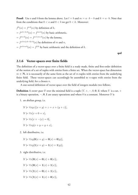
Pro<strong>of</strong>: Use a and b from <strong>the</strong> lemma above. Let l = b and m = a · b − b and k = a · b. Note that<br />
from <strong>the</strong> conditions that 0 < a and 0 < b we get 0 < k. Moreover:<br />
f k (α) = f a·b (α) by definition <strong>of</strong> k,<br />
= f a·b−b+b (α) = f m+b (α) by basic arithmetic,<br />
= f m+b (α) = f a·l+m+b (α) by <strong>the</strong> lemma,<br />
= f a·b+(a·b−b)+b (α) by definition <strong>of</strong> m and n,<br />
= f a·b+a·b (α) = f 2·k by basic arithmetic and <strong>the</strong> definition <strong>of</strong> k.<br />
2.1.6 Vector-spaces over finite fields<br />
The definition <strong>of</strong> a vector-space over a finite field is a ready made, finite and first-order definition<br />
<strong>of</strong> <strong>the</strong> notion <strong>of</strong> a set <strong>of</strong> tuples with entries from a finite set. When <strong>the</strong> vector-space has dimension<br />
m ∈ N, it is necessarily <strong>of</strong> <strong>the</strong> same form as <strong>the</strong> set <strong>of</strong> m-tuples with entries from <strong>the</strong> underlying<br />
finite field. These vector-spaces can accordingly be assembled to n-tapes with entries from <strong>the</strong><br />
underlying field, for a chosen n.<br />
A one-sorted definition <strong>of</strong> vector space over <strong>the</strong> field <strong>of</strong> integers modulo two follows.<br />
Definition A vector space V over <strong>the</strong> minimal field is a tuple (V, +, −, 0, 0, 1) where V is a set, +<br />
is a binary operation, −, 0, 1 are unary operations and where 0 is a constant. Moreover V is<br />
1. an abelian group, i.e.<br />
V |= ∀xyz[(x + y) + z = x + (y + z)],<br />
V |= ∀x[x + 0 = x],<br />
V |= ∀x[x + −(x) = 0],<br />
V |= ∀xy[x + y = y + x],<br />
2. left distributive, i.e.<br />
V |= ∀xy[0(x + y) = 0(x) + 0(y)],<br />
V |= ∀xy[1(x + y) = 1(x) + 1(y)],<br />
3. right distributive, i.e.<br />
V |= ∀x[0(x) = 0(x) + 0(x)],<br />
V |= ∀x[0(x) = 1(x) + 1(x)],<br />
V |= ∀x[1(x) = 0(x) + 1(x)],<br />
V |= ∀x[1(x) = 1(x) + 0(x)],<br />
qed<br />
42