n ypy

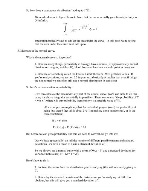
So how does a continuous distribution “add up to 1”??
We need calculus to figure this out. Note that the curve actually goes from (-)infinity to
(+)infinity:
∞
1
∫ 2
e−1 2 y−
2
dy = 1
−∞
Integration basically says to add up the area under the curve. In this case, we're saying
that the area under the curve must add up to 1.
5. More about the normal curve.
Why is the normal curve so important?
1. Because many things, particularly in biology, have a normal, or approximately normal
distribution: heights, weights, IQ, blood hormone levels (at a single point in time), etc.
2. Because of something called the Central Limit Theorem. Well get back to this. If
you’re really curious, see section 6.2 in your text (basically it implies that even if things
are not normal we can often still use a normal distribution in statistics).
So here’s our connection to probability:
- we can calculate the area under any part of the normal curve, (we'll use table to do this -
using the above integral is essentially impossible). Then we can say “the probability of Y
< y is x”, where x is our probability (remember y is a specific value of Y).
- For example, we might say that for basketball players (men) the probability of
being less than 6 feet tall is about 5% (I’m making these numbers up), or in the
correct notation:
if y = 6, then
Pr(Y < y) = Pr(Y < 6) = 0.05
But before we can get a probability like this we need to convert our y's into z's:
Our y's have (potentially) an infinite number of different possible means and standard
deviations. z's have a mean of 0 and a standard deviation of 1.
So we always use a normal curve with a mean of 0 (μ = 0) and a standard deviation (or
variance in this case) of 1 (σ = 1 = σ 2 ).
Here’s how to do it:
1. Subtract the mean from the distribution you’re studying (this will obviously give you
0).
2. Divide by the standard deviation of the distribution you’re studying. A little less
obvious, but this will give you a standard deviation of 1.