VIII. Addition of Angular Momenta
VIII. Addition of Angular Momenta
VIII. Addition of Angular Momenta
You also want an ePaper? Increase the reach of your titles
YUMPU automatically turns print PDFs into web optimized ePapers that Google loves.
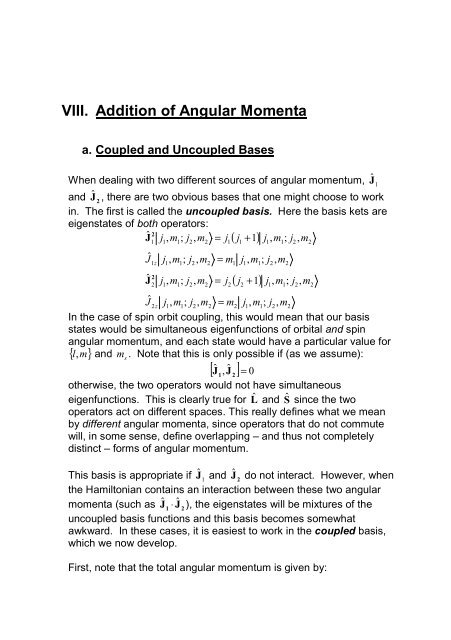
<strong>VIII</strong>. <strong>Addition</strong> <strong>of</strong> <strong>Angular</strong> <strong>Momenta</strong><br />
a. Coupled and Uncoupled Bases<br />
When dealing with two different sources <strong>of</strong> angular momentum, Ĵ 1<br />
and Ĵ 2<br />
, there are two obvious bases that one might choose to work<br />
in. The first is called the uncoupled basis. Here the basis kets are<br />
eigenstates <strong>of</strong> both operators:<br />
2<br />
Ĵ 1 1 1 1 1 1<br />
j , m ; j 2<br />
, m 2<br />
= j ( j + 1) j , m 1<br />
; j 2<br />
, m 2<br />
Ĵ 1z<br />
j 1<br />
, m 1<br />
; j 2<br />
, m 2<br />
= m 1<br />
j 1<br />
, m 1<br />
; j 2<br />
, m 2<br />
2<br />
Ĵ 2 1 1 2 2 1 1<br />
j , m ; j 2<br />
, m 2<br />
= j ( j + 1) j , m ; j 2<br />
, m 2<br />
Ĵ 2 z<br />
j 1<br />
, m 1<br />
; j 2<br />
, m 2<br />
= m 2<br />
j 1<br />
, m 1<br />
; j 2<br />
, m 2<br />
In the case <strong>of</strong> spin orbit coupling, this would mean that our basis<br />
states would be simultaneous eigenfunctions <strong>of</strong> orbital and spin<br />
angular momentum, and each state would have a particular value for<br />
{ l , m } and m<br />
s<br />
. Note that this is only possible if (as we assume):<br />
[J ˆ , Jˆ<br />
1 2<br />
]= 0<br />
otherwise, the two operators would not have simultaneous<br />
eigenfunctions. This is clearly true for L ˆ and Ŝ since the two<br />
operators act on different spaces. This really defines what we mean<br />
by different angular momenta, since operators that do not commute<br />
will, in some sense, define overlapping – and thus not completely<br />
distinct – forms <strong>of</strong> angular momentum.<br />
This basis is appropriate if Ĵ 1<br />
and Ĵ 2<br />
do not interact. However, when<br />
the Hamiltonian contains an interaction between these two angular<br />
momenta (such as Ĵ 1<br />
⋅ Ĵ 2<br />
), the eigenstates will be mixtures <strong>of</strong> the<br />
uncoupled basis functions and this basis becomes somewhat<br />
awkward. In these cases, it is easiest to work in the coupled basis,<br />
which we now develop.<br />
First, note that the total angular momentum is given by:
J ˆ = J ˆ<br />
1<br />
+ J ˆ<br />
2<br />
It is easy to show that this is, in fact, an angular momentum (i.e.<br />
[J ˆ , Jˆ y<br />
]= i Jˆ<br />
). We can therefore associate two quantum numbers, j<br />
x<br />
z<br />
and m , with the eigenstates <strong>of</strong> total angular momentum indicating its<br />
magnitude and projection onto the z axis. The coupled basis states<br />
are eigenfunctions <strong>of</strong> the total angular momentum operator. This<br />
specifies two quantum numbers for our basis states ( j and m ).<br />
However, as we saw above, the uncoupled basis states were<br />
specified by four quantum numbers ( j<br />
1<br />
, j 2<br />
, m 1<br />
and m 2<br />
) and we<br />
therefore need to specify two more quantum numbers to fully specify<br />
the coupled states. To specify these last two quantum numbers, we<br />
note that<br />
2<br />
[J ˆ , Jˆ<br />
ˆ 2 ˆ ˆ 2<br />
1 z<br />
]= [(J + 2 J ˆ<br />
1<br />
⋅ J + J 2<br />
), J ˆ ]= [2 J ˆ<br />
1<br />
⋅ J ˆ<br />
2<br />
, Ĵ ]= 2 [J ˆ 1, Jˆ 1 z<br />
]⋅ J ˆ<br />
1 2 1 z 1 z 2<br />
≠ 0<br />
and similarly for Ĵ 2 z<br />
. Thus Ĵ 1 z<br />
and Ĵ 2 z<br />
do not share common<br />
eigenfunctions with J ˆ 2 . To put it another way, to obtain a definite<br />
state <strong>of</strong> the total angular momentum, one must generally mix states<br />
with different m 1<br />
and m 2<br />
. All thus leads to the conclusion that neither<br />
m 1<br />
nor m 2<br />
can be one <strong>of</strong> the other quantum numbers that specify the<br />
coupled basis.<br />
What about j<br />
1<br />
and j<br />
2<br />
? Well,<br />
2<br />
[ J ˆ 2, J ˆ ]= [(J ˆ 2 + 2 J ˆ 2 ˆ 2 2 ˆ 2<br />
1<br />
⋅ J ˆ + J ˆ<br />
2<br />
), J ]= [2 J ˆ<br />
1<br />
⋅ J ˆ , J ˆ ˆ<br />
1<br />
]= 2 [ˆ J , 1 1 2 1 2 1<br />
J<br />
1<br />
]⋅ J<br />
2<br />
≠ 0<br />
2<br />
and similarly for J ˆ<br />
2<br />
. Further<br />
2 ˆ 2 ˆ ˆ 2<br />
[Ĵ , J ˆ<br />
z 1<br />
]= [Ĵ<br />
1 z<br />
+ Ĵ 2 z<br />
, J<br />
1<br />
]= [J<br />
1 z<br />
, J 1<br />
]≠ 0 .<br />
2 2<br />
Hence, J ˆ 2 , Ĵ z<br />
, J ˆ and J ˆ<br />
1<br />
2<br />
share common eigenfunctions, and these<br />
eigenfunctions define the coupled basis. To say it another way, the<br />
eigenstates <strong>of</strong> J ˆ 2 do not mix states with different j<br />
1<br />
and j 2<br />
. This is<br />
rather pr<strong>of</strong>ound – in the case <strong>of</strong> spin-orbit coupling it means that<br />
states with different values <strong>of</strong> l will not be mixed by the coupling.<br />
The appropriate quantum numbers for the coupled basis are j , m , j 1<br />
and j and we have:<br />
2
J ˆ 2 j,m; j<br />
1, j<br />
2<br />
= j( j + 1) j,m; j<br />
1, j2<br />
Ĵ j,m; j , j = m j,m; j , j<br />
z 1 2 1 2<br />
2<br />
J ˆ<br />
1<br />
j,m; j 1<br />
, j 2<br />
= j 1<br />
( j 1<br />
+ 1) j,m; j 1<br />
, j 2<br />
2<br />
J ˆ<br />
2<br />
j,m; j 1<br />
, j 2<br />
= j 2<br />
( j 2<br />
+ 1) j,m; j 1<br />
, j 2<br />
Typically, certain matrix elements will be easier to compute in the<br />
coupled basis, while others will be easier to compute in the<br />
uncoupled basis. Thus, we will <strong>of</strong>ten need to transform from one<br />
basis to the other. Since the coupled and uncoupled bases are both<br />
eigenfunctions <strong>of</strong> Hermitian operators, each forms a complete basis<br />
for the angular momentum and therefore we can write:<br />
j,m; j , j = j ',<br />
m ; j ',<br />
m j ',<br />
m ; j ',<br />
m j,m; j , j .<br />
1 2 1 1 2 2 1 1 2 2 1 2<br />
j 1 ',<br />
m 1<br />
j 2 ',<br />
m 2<br />
However, we have already concluded that J ˆ 2 does not mix states<br />
with different j<br />
1<br />
and j<br />
2<br />
so:<br />
j<br />
1' , m<br />
1; j<br />
2<br />
',<br />
m<br />
2<br />
j,m; j<br />
1, j<br />
2<br />
= j<br />
1,m 1<br />
; j 2<br />
,m<br />
2<br />
j,m; j<br />
1, j<br />
2<br />
δ j , j<br />
δ<br />
1 1 ' j2 , j 2 '<br />
As a result the sums over j<br />
1' and j<br />
2' collapse to delta functions and<br />
we get:<br />
j,m; j , j = j ,m ; j 2<br />
,m 2<br />
j ,m ; j 2<br />
,m 2<br />
j,m; j , j<br />
1 2 1 1 1 1 1 2<br />
m 1 ,m 2<br />
The transformation coefficients j<br />
1,m 1<br />
; j 2<br />
,m<br />
2<br />
j,m; j<br />
1, j<br />
2<br />
are known as<br />
the Clebsch-Gordon (CG) coefficients (or the vector coupling<br />
coefficients). The CG matrix is unitary (since it just transforms a<br />
vector from one basis to another) and by convention its elements are<br />
chosen real (recall that the phase <strong>of</strong> j,m; j 1<br />
, j<br />
2<br />
is arbitrary).<br />
There is one additional symmetry that the CG coefficients possess.<br />
Notice that:<br />
ˆ ˆ ˆ<br />
0 = (m − J ) j,m; j , j = (m − J 1z<br />
− J 2 z<br />
) j,m; j , j<br />
z 1 2 1 2<br />
0 = j ,m ; j ,m 2<br />
(m − Jˆ<br />
1z<br />
− J ˆ<br />
2 z<br />
) j,m; j , j<br />
1 1 2 1 2<br />
0 = (m − m<br />
1<br />
− m 2<br />
) j<br />
1<br />
,m 1<br />
; j 2<br />
,m 2<br />
j,m; j<br />
1, j2<br />
This implies that either the CG coefficient is zero, or
m = m 1<br />
+ m 2<br />
.<br />
Thus, for all the non-zero CG coefficients, the index m is actually<br />
redundant; it is always given by the sum <strong>of</strong> m 1<br />
and m 2<br />
.<br />
b. Recursion Relations<br />
There are several ways to determine the CG coefficients. Perhaps<br />
the easiest is to look them up in a book (they have been extensively<br />
tabulated). However, this method is the most prone to error, unless<br />
you are very careful to follow all <strong>of</strong> the sign conventions <strong>of</strong> the text at<br />
hand (which may not be the same as the sign conventions in, say<br />
CTDL or these lecture notes).<br />
Another route is to simply view the whole thing as an eigenvalue<br />
problem: one simply wishes to determine the eigenstates <strong>of</strong> J ˆ 2 in the<br />
uncoupled basis. The coefficients <strong>of</strong> the different eigenvectors are<br />
the CG coefficients. However, this misses out on what is probably<br />
the most important aspect <strong>of</strong> angular momentum coupling – the ability<br />
without any significant computation to predict the allowed<br />
quantum numbers and their degeneracies.<br />
We will follow a third route to obtain the CG coefficients. This notes<br />
that the coefficients are easily obtained by recursion, in a manner<br />
similar to what we used for the spherical harmonics. First we note<br />
that there is only one non-zero coefficient for m = m + m max 1max 2max<br />
:<br />
j 1<br />
, m 1max<br />
; j 2<br />
, m 2max<br />
j, m max<br />
; j 1<br />
, j 2<br />
. No other combination <strong>of</strong> m 1<br />
and m 2<br />
will give the correct total m . Thus, the states j, m<br />
max<br />
; j<br />
1<br />
, j<br />
2<br />
and<br />
j<br />
1<br />
, m<br />
1max<br />
; j 2, m 2max<br />
are equal up to an unimportant constant. By<br />
convention, this constant is chosen to be 1. We can generate the<br />
other coefficients by successive applications <strong>of</strong> the lowering operator<br />
and judicious use <strong>of</strong> orthogonality constraints.<br />
To see how this is applied in practice, it is best to use spin-orbit<br />
coupling as an example. What is the coupled basis for a spin-1/2<br />
electron with orbital angular momentum l ? We can identify the<br />
uncoupled quantum numbers:
j = l<br />
m 1<br />
= m l<br />
1<br />
1<br />
j 2<br />
= s = 2<br />
m 2<br />
= m s<br />
ˆ 2<br />
ˆ<br />
And we want to determine the eigenstates <strong>of</strong> Ĵ 2 ≡ ( L + S) and<br />
J ˆ = L ˆ + S ˆ<br />
z z z<br />
. We know now that the two states with maximum m are<br />
equal:<br />
Coupled: Uncoupled:<br />
1 1<br />
l + 1 2<br />
, m = l + 2<br />
; l , s = l , m l<br />
= l ; s , + 2<br />
.<br />
Applying the lowering operator, we have<br />
1<br />
J l + 1 , m = l + 1 ; l , s = ( J ˆ + J ˆ<br />
2 l − s −<br />
) l , m = l ; s , + 2<br />
ˆ<br />
− 2 l<br />
1<br />
)( l<br />
= ( l + l l − + 1 ) l , l − 1 ; s , +<br />
2 1 + ( s + 1 )( s − + 1 ) l , l ; s , −<br />
2 2<br />
1 1<br />
= 2 l l , l − 1 ; s , + 2<br />
+ l , l ; s , − 2<br />
However, we also know that<br />
1 1 1<br />
J ˆ<br />
−<br />
l + 1 , m = l + 1 1<br />
2<br />
; l , s = ( l + + l +<br />
2 )( l + − l −<br />
2 + 1 ) l + 1<br />
2 2 2 2<br />
, m = l −<br />
2 1 ; l , s<br />
= 2 l + 1 l + 1 , m = l − 1 2 2<br />
; l , s<br />
Combining these last two expressions,<br />
2 l 1<br />
1 1<br />
l + 1 1<br />
2<br />
, m = l − 2<br />
; l , s = l , l − 1 ; s , + 2<br />
+ l , l ; s , − 2<br />
2 l + 1 2 l + 1<br />
This gives us the expression for the state with the same j , l and s<br />
but m = m<br />
max<br />
− 1 . One can check that this state is normalized. We<br />
can clearly apply this recursively to obtain the states with<br />
m = m<br />
max<br />
− 2 , m = m<br />
max<br />
− 3 , etc. Clearly this will cease when<br />
1<br />
m = − l − 2<br />
= m mi n<br />
.<br />
To get some insight into what these states look like, we need to make<br />
our notation a little less explicit, temporarily. First we will delete the<br />
indices for l and s from all the bra and ket states since these<br />
quantum numbers are the same throughout the calculation. So, for<br />
example, j , m ; l , s → j , m and l , m l<br />
; s , m s<br />
→ m l<br />
; m s<br />
Second, in terms<br />
<strong>of</strong> the abbreviated state labels, we will write the above relationship<br />
symbolically<br />
1 1 1 1<br />
l + 1 , l − 2<br />
≈ l + 1 2 2<br />
, l − 2<br />
≈ l − 1 ; +<br />
2<br />
+ l ; − 2<br />
where ≈ means roughly “neglecting any constants that are not<br />
relevant for the point I want to make”. In this case, they are factors<br />
1<br />
2
involving l and s that will be very important for doing calculations but<br />
impede our understanding at the outset.<br />
Using this notation, we can write the next lowered state:<br />
3<br />
l + 1 , l − 2<br />
≈ Ĵ −<br />
l + 1 1<br />
, l − 2<br />
≈ ( Jˆ<br />
1<br />
J ˆ l − 1 ; + + Jˆ<br />
+ Jˆ<br />
l;<br />
−<br />
) ( )<br />
2 2 l −<br />
+<br />
s −<br />
2 l−<br />
s−<br />
1<br />
2<br />
≈<br />
l − 2 ; +<br />
1<br />
2<br />
+<br />
l − 1 ; −<br />
In fact, if we make rows <strong>of</strong> each <strong>of</strong> the coupled states we can make a<br />
flow chart for the different components:<br />
1<br />
≈ l;<br />
2<br />
l + 1 , l + 2<br />
1<br />
+<br />
2<br />
1<br />
2<br />
1<br />
l + 1 1<br />
, l − 2<br />
≈ l − 1 ; +<br />
2<br />
+ l; −<br />
1<br />
2 2<br />
1<br />
l + 1 3<br />
, l − 2<br />
≈ l − 2 ; +<br />
2<br />
+ l − 1 ; −<br />
. . .<br />
2<br />
1 1 1<br />
l +<br />
2<br />
, − l +<br />
2<br />
≈ − l; +<br />
2<br />
+ − l + 1 ; −<br />
1<br />
2<br />
1<br />
2<br />
1 1<br />
l + 1 2<br />
, l − 2<br />
≈ − l; −<br />
2<br />
So we see that the characteristic action <strong>of</strong> the lowering operator is to<br />
connect upper states in ( m<br />
l<br />
, m<br />
s<br />
) space to states that are below and to<br />
the right <strong>of</strong> the original state. This action is limited by the fact that<br />
m l<br />
cannot be less than − l (this determines the “height” <strong>of</strong> the ladder)<br />
and m cannot be less than − 1 2<br />
(this determines the widths <strong>of</strong> the<br />
s<br />
rungs).<br />
c. The triangle rule<br />
So, have we now created all the coupled states? Well, the total<br />
number <strong>of</strong> coupled states in the ladder is 2 j + 1 = 2 ( l + 1 ) = 2 l + 2 .<br />
2
Meanwhile, the number <strong>of</strong> uncoupled states is<br />
( 2 l + 1)( 2s<br />
+ 1) = ( 2l<br />
+ 1) 2 = 4l<br />
+ 2 . Since the number <strong>of</strong> coupled and<br />
uncoupled states must be equal, we are missing 2 l states. To find<br />
the missing states, notice that all <strong>of</strong> the above states have j = l +<br />
2 1 .<br />
That is, we have presumed that l and s point in the same direction<br />
(equivalently, we have presumed that they are rotating in the same<br />
plane an in the same sense – clockwise or counterclockwise). This is<br />
clearly an unnecessary restriction. Hence, we expect there to be<br />
another possibility for j - specifically, in order to account for all the<br />
“missing” states, we expect 2 j + 1 = 2l<br />
, or j = l −<br />
2 1 .<br />
To build these missing states, we note that there are two uncoupled<br />
functions with m = m − max<br />
1 : m l −1 ; m =<br />
2 1 and m l; m = −<br />
2 1 .<br />
l<br />
=<br />
s<br />
l<br />
=<br />
s<br />
Meanwhile, we have only found one coupled state m l −1 ; m +<br />
2 1 :<br />
j = l + 1<br />
; m = l −<br />
2<br />
1<br />
2<br />
l<br />
=<br />
s<br />
. Based on the above arguments, we predict there<br />
will also be a state j = l − 1<br />
; m = l −<br />
1<br />
2<br />
2<br />
. To find it we note that 1) this<br />
state must be a linear combination <strong>of</strong> m l −1 ; m =<br />
2 1 and<br />
m<br />
l<br />
l; m = − 1<br />
=<br />
s<br />
2<br />
l<br />
=<br />
s<br />
, since other states do not conserve m 2) the new<br />
state must be orthogonal to the j = l + 1<br />
; m = l −<br />
2 1<br />
2<br />
, since both states<br />
2<br />
are eigenstates <strong>of</strong> the same operator ( Ĵ ). Using our explicit<br />
expression for j = l + 1<br />
2<br />
; m = l −<br />
2 1 (above), it is easy to show that the<br />
normalized state satisfying 1) and 2) is:<br />
1<br />
2l<br />
1<br />
1<br />
1<br />
l −<br />
2<br />
1 , m = l −<br />
,<br />
2<br />
; l,<br />
s = l,<br />
l −1;<br />
s,<br />
+<br />
2<br />
− l,<br />
l;<br />
s −<br />
2<br />
2l<br />
+ 1<br />
2l<br />
+ 1<br />
where we have once again made an arbitrary choice <strong>of</strong> phase, so that<br />
the coefficient <strong>of</strong> the first term is positive. Starting from this state, we<br />
can apply the lowering operator recursively to generate the 2 l states<br />
1<br />
l − , m;<br />
l,<br />
s with all other possible values <strong>of</strong> m .<br />
2<br />
How do these ladders generalize to arbitrary m<br />
1<br />
and m<br />
2<br />
? Well, one<br />
finds that the possible values <strong>of</strong> j fall between two limits:<br />
j<br />
1<br />
− j2<br />
≤ j ≤ j1<br />
+ j2<br />
This may be familiar to some <strong>of</strong> you as the “triangle rule” <strong>of</strong> angular<br />
momentum coupling. Physically, this comes from the fact that the<br />
maximum number <strong>of</strong> states we can have with a given m is 2 j 2<br />
+ 1
(assuming j<br />
1<br />
> j2<br />
). Pictorially, this corresponds to the maximum width<br />
<strong>of</strong> the “rungs” on our ladder. Now, when we write out a table <strong>of</strong> the<br />
m values for each j , we find:<br />
j=j 1 +j 2 j=j 1 +j 2 -1 j=j 1 +j 2 -2 j=j 1 +j 2 -3<br />
m= j 1 +j 2 X<br />
m=j 1 +j 2 -1 X X<br />
m=j 1 +j 2 -2 X X X<br />
m=j 1 +j 2 -3 X X X X<br />
… X X X X<br />
m=-j 1 -j 2 +3 X X X X<br />
m=-j 1 -j 2 +2 X X X<br />
m=-j 1 -j 2 +1 X X<br />
m=-j 1 -j 2 X<br />
We see that having n different values for j requires us to have n<br />
different states with a given value <strong>of</strong> m . For example, in the chart<br />
above, we would need four states with m=j 1 +j 2 -3 to support the four<br />
values <strong>of</strong> j that are listed. Since the maximum degeneracy <strong>of</strong> each<br />
m level is 2 j 2<br />
+ 1, there are 2 j 2<br />
+ 1 possible values <strong>of</strong> j and we<br />
conclude that they are j<br />
1<br />
− j2<br />
≤ j ≤ j1<br />
+ j2<br />
.<br />
We can also check that the number <strong>of</strong> states predicted by the triangle<br />
rule agrees with what we know from the uncoupled basis. For each<br />
value <strong>of</strong> j we have 2 j + 1 states, so the total number <strong>of</strong> states is (if<br />
we assume that j<br />
1<br />
> j2<br />
):<br />
( 2(<br />
j<br />
1<br />
+ j2<br />
) + 1) + ( 2( j1<br />
+ j2<br />
−1)<br />
+ 1) + ... + ( 2( j1<br />
− j2<br />
+ 1) + 1) + ( 2( j1<br />
− j2<br />
) + 1)<br />
.<br />
Or, rearranging the terms,<br />
( 2 j1 1) + 2 j2<br />
+ ( 2 j1<br />
+ 1) + 2 j2<br />
− 2 + ... + ( 2 j1<br />
+ 1) − 2 j2<br />
+ 2 + ( 2 j1<br />
+ 1) − 2 j2<br />
+ .<br />
The terms outside the parentheses clearly sum to zero. Meanwhile,<br />
there are exactly 2 j 2<br />
+ 1 copies <strong>of</strong> the term in parentheses. Hence,<br />
the number <strong>of</strong> states is<br />
( 2 j<br />
1<br />
+ 1)( 2 j2<br />
+ 1)<br />
which is precisely the number <strong>of</strong> states in the uncoupled<br />
representation.


