Scalable 2d Convex Hull and Trianglulation Algorithms for Coarse ...

Scalable 2d Convex Hull and Trianglulation Algorithms for Coarse
Grained Mult ieomput ers
Afonso Ferreira* Andrew Rau-Chaplint Stkphane Ukdat
LIP ENS-Lyon Technical University of Nova Scotia LIP ENS-Lyo11
46, allke d’Italie P.O. Box 1000, 46, all& d’Italie
69364 Lyon Cedex 7 Halifax, Nova Scotia 69364 Lyon Cedex
France Canada B3J 2x4 France
Absract
In this paper we describe scalable parallel algorithms
for building the Convex Hull and a Triangulation of
a given point set in R2. Theae algorithms are designed
for the coarse rained multicomputer model:
p processors with O(gf >> O(1) local memory each,
connected to som,e arbitrary interconnection network
(e.g. mesh,, hypercube, omega). They require time
O( Tseqyntiai + T,(n,p)), where Ts(n,p) refers to the
time of a global sort of n data on a p processor machine.
Furthermore, they involve only a constant number
of global communication rounds. Since computing
either 2d Convex Hull or Trian!gulation requires time
Tsequential = @(TI log n) these algorithms either run in
optimal time, e(?), or in sort time, ~.(n,p), for
the interconnection network in question. These results
become optimal when T8e9yntiai. dominates T, (n, p),
for instance when randomized sorting algorithms are
used, or for interconnection networks like the mesh for
which optimal sorting algorithms exist.
1 Introduction
Most existing multicomputers (e.g. the Intel
Paragon, Cray T3D, Meiko CS-:2 and IBM SP2) consist
of a set of p state-of-the-art processors, each with
considerable local memory, connected to some interconnection
network (e.g. mesh, hypercube, omega).
These machines are usually coarse grained, i.e. the
size of each local memory is “considerably larger” than
O(1). Despite this fact, most theoretical parallel algorithms,
in particular those for solving geometric problems,
assume a fine grained setting, where a problem
of size n is to be solved on a parallel computer with p
processors (e.g., a PRAM, mesh, or hypercube multiprocessor)
such that 2 = O(1). However, as noted in
* (ferreira@lip.ens-lyon.fr) Partially supported by the project
Stratageme of the French CNRS and by DRET
t (arc@tuns.ca) Partially supported by DIMACS, a National
Science Foundation center (USA), and the Natural Sciences and
Engineering Research Council (Canac a).
* (ubeda@lip.ens-lyon.fr) Partially supported by the project
PRS (CAPA) of the French CNRS
[9], to be relevant in practice such algorithms must be
scalable, that is, they must be applicable and efficient
for a wide range of ratios E.
P
In this paper we describe scalable parallel algorithms
for some fundamental geometric problems.
Among the first scalable coarse grained algorithms
for solving geometric problems on distributed memory
machines were described in [6]. The majority of these
algorithms were optimal on architectures for which
optimal sorting algorithms were known and reciuired
at most sort time otherwise. Another important feature
of these algorithms was that they involved only
a constant number of global communication rounds,
which had the effect of malting them very fast in
practice. Problems studied in [6] included computing
the area of the union of rectangles, 3D-maxima, 2Dnearest
neighbors of a point set, and lower envelope
of non-intersecting line segments in the plane. All of
these algorithms used. a spatial partioning technique
in which a constant number of partitioning schemes
of the global problem (on the entire data set of 12
data items) into p subproblems of size O( %) were used.
Each processor solved (sequentially) a constant number
of such O($) size subproblems, and a const>ant
number of global routing operations were used to permute
the subproblems between the processors. Eventually,
by combining the O(1) solutions of its O($)
size subproblems, each processor determined its O( $)
size portion of the global solution.
For most of the problems addressed in [6] the spatial
partitioning technique described above were very
efficient. One exception was the 2d Convex Hull
problem for which the resulting algorithm required
+ Ts(n,p) + logpTs(p,p)) time and involved
O ( y
logp global communication rounds. Subsequent work
on this problem has focussed on developing randoniized
algorithms that trade-off guaranteed solutions for
efficiency (i.e. a constant number of commnnication
rounds). In [7] Deng and Gu solve the 2d convex h~dl
problem with high probability for any input assuming
E > p2+€ while Dehne, Kenyon and Fabri solve for a
p. -
given a set of “well distributed inputs” the lid convex
1063-6374195 $04.00 0 1995 IEEE
561

hull problem, for any constant L, and 2 p‘.
In this paper we describe a deterministic scalable
algorithm for solving the 2d convex hull problem on
the coarse grained multicomputer model: p processors
with O(n) >> O(1) local memory each, connected to
P
some arbitrary interconnection network. Our algorithmrequires
time O(F+T,(n,p)), whereT,(n,p)
refers to the time of a global sort of n data on a p processor
machine. Furthermore, it involves only a constant
number of global communication rounds. Based
on this algorithm we also give an algorithm for solving
the triangulation problem for points in R2 for the
same model and in the same space and time.
Since computing either 2d convex hull or triangulation
requires time Tseguential = O(n log n) [14]
our algorithms either run in optimal time e(*)
or in sort time T,(n,p) for the interconnection net-
work in question. Our results become optimal when
T3 e *” e n t I a I
dominates T,(n,p), for instance when ran-
P
domized sorting algorithms are used, or when T,(n,p)
is optimal.
Consider, for example, the mesh architecture. For
the fine grained case (; = O(l)), a time complexity of
O( fi) is optimal. Hence, simulating the existing fine
grained results on a coarse grained machine via Brent’s
Theorem [ll] leads to a O($& time coarse grained
method. Our algorithmruns in time O(:(logn+fi)),
a considerable improvement over both simulation and
the existing methods.
The Coarse Grained Multicom uter model, or
CGM(n,p) for short, is defined in b]. It consists of
a set of p processors with O($) local memory each,
connected to some arbitrary interconnection network
or a shared memory. The term “course graine8’ refers
to the fact that (as in practice) the number of words
of each local memory O(;) is defined to be “considerably
larger” than O(1). Our definition of “considerably
larger” (and the one used in [SI) is that : 2 p.
This is clearly true for all currently available coarse
grained parallel machines. In the following, all messages
are composed of a constant number of words
and, for determining time complexities, we will consider
both local computation time and inter processor
communication time in the standard way.
For the problems studied in this paper, we are interested
in algorithms which are optimal or at least
efficient for a wide range of ratios 2. We present a
new technique for designing efficient scalable parallel
geometric algorithms. Our results are independent of
the communication network (e.g. mesh, hypercube, fat
tree). A particular strength of this approach (which
is very different from the one presented in [l, SI), is
that all inter processor communication is restricted to
a constant number of usages of a small set of simple
communication operations. This has the effect of making
the algorithms both easy to implement in that all
communications is performed by calls to a standard
highly optimized communication library and very fast
P
in practice (see [6] for evidence of this).
Our Convex Hull algorithm is described below and
has the following basic structure. The entire data set
for a given problem is assumed to be initially distributed
into the local memories and remains there
until the problem is solved. Given a set S of n points
and a p processor coarse grained multicomputer we
show how to compute the upper hull of S. The lower
hull, and therefore the complete hull, can be computed
analogously. In the remainder we assume without loss
of generality that all points are in the first quadrant.
Upper Hull(S)
[nput: Each processor stores a set of points drawn arbixarily
from S.
Dutput: A distributed representation of upper hull of S. All
Joints on the upper hull are identified and labeled from left
.o right.
1. Globally sort the points in S by x-coordinate. Let S, denote
the set of 2 sorted points now stored on processor
2.
2. Independently and in parallel, each processor i computes
the upper hull of the set S;. Let X ; denote the result on
processor i.
3. By means of a merge operation compute for each upper
hull X;, 1 < i 5 p, the upper common tangent line between
it and all upper hulls X, , i < j < p, and label the
upper hull of S by using the upper tangent lines.
Step 1 of algorithm UpperHull(S) can be completed
by using a global sort operation as described in Section
2. Step 2 is a totally sequential step and can be
completed in time O( F) using well known sequential
methods [14]. The main challenge is in performing
Step 3. This step amounts to a merge algorithm
in which p disjoint upper hulls are merged into a single
hull. We present two different merge procedures:
MergeHullsl and MergeHulls2. The first, described
in Section 3.3, is a straightforward merge requiring a
constant number of global communication rounds and
11 > p2 local memory per processor. The second merge
P -
procedure (MergeHulls2), described in Section 3.4, is
a more complex merge that uses the first merge as
a subprocedure but has a higher degree of scalability
in that it requires only that 3 > p while still requir-
P -
ing only a constant number of communication rounds.
Both algorithms use the idea of selecting splitter sets
which was introduced in the context of solving convex
hulls by Miller and Stout [13].
Our algorithm for triangulating n points in R2 is
based on our convex hull algorithm and the observation
that a set S of points can be triangulated by first
triangulating x-disjoint subsets from S and then triangulating
the regions between the convex hulls formed
by these triangulated regions, which is a simpler subproblem
as these regions belong to a class of simple
562

polygons called funnel polygons [ 161.
The remainder of this paper is organized as follows:
in the next section we give more details about
the coarse grained multicomputer model, CGM(n, p).
Section 3 presents our Upper Hull algorithm, whi e
Section 4 describes how the Upper Hull algorithm can
be adapted to solve the triangulaiion problem. In section
5 we conclude.
2 The Coarse Grained Model: Definitions
and Basic Operations
The Coarse Grazned Multzcomputer, CGM(n,p),
considered in this paper is a set (of p processors numbered
from 1 to p with O(%) local memory each, connected
via some arbitrary interconnection network or
a shared memory. Commonly used interconnection
networks for a CGM include the 2D-mesh e.g. Intel
Paragon), hypercube (e.g. Intel iPSC/S60\ and the
fat tree (e.g. Thinking Machine,; CM-5). For determining
time complexities, we limit all messages to a
constant number of words and account for both local
computation time and inter processor communication
time. The term “coarse grained” refers to the fact
that the size O(:) of each local memory will typically
be “considerably larger” than 0 (1). We will assume
either > p as was assumed in [6].
P -
Global sort refers to the operation of sorting O(n)
data items stored on a CGM(n,p), O(f) data items
per processor, with respect to the CGiWs processor
numbering. T,(n,p) refers to the time complexity of
a global sort.
Note that, for a mesh T,(n,p) = O($(logn + Jis))
and for a hypercube T,(n,p) = O(:(logn
+ log’p)).
These time complexities are based on [2] and [12], respectively.
Note that for the h,ypercube an asymptotically
better deterministic algorithm exists [4], but
it is of more theorical than practical interest. One
could also use randomized sorting [15], but in this paper
we will focus primarily on deterministic methods.
We refer the reader to [2, 3, 10, 3 1, 12, 151 for a more
detailed discussion of the different architectures and
routing algorithms.
We will now outline four other operations for interprocessor
communication which will be used in the
remainder of this paper. All of these operations can
be implemented as a constant number of global sort
operations and O(:) time local computation. Note
that, for most interconnection networks it would be
better in practice to implement these operations directly
rather than using global sort as this would typically
improve the constants in the time complexity of
the algorithms described in the remainder.
Segmented broadcast: In a segmented broadcast operation,
q < p processors with numbers j, < j~ <
... < j, are selected. Each such processor, p,, , broad-
casts a list of 1 5 k < :
data items from its local
memory to the processors p3,+1 . ..p3,+,-1. The time
for a segmented broadcast operation will be referred
to 8s T.b(k,p)-
Segmented gather: In a segmented gather operation,
q 5 p processors with ids j, < j2 < . . . < j, are
selected. Each such processor, pj;, is sent a data item
from processorspj,+l . . . pj,,, -1. This operation is the
inverse of a segmented broadcast. Note that care must
be taken to ensure that the selected processors have
enough memory to receive all sent messages. The time
for a se mented gather operation will be referred to as
TS,(k,P5.
All-to-All broadcast: In an All-to-All broadcast operation,
every processor sends one message to all other
processors. The time complexity will be denoted as
Ta2a (P).
Personalized All-to-.All broadcast: In a Personalized
All-to-All broadcast operation, every processor sends
a different message to every other processor. The time
complexity will be denoted as Tpa2a(n,p).
Partial sum (Scan): Every processor stores one
value, and all processors compute the partial sums of
these values with respect to some associative operator.
The time complexity will be denoted as Tps(n,p).
For any CGM(n,p) with 2 p it is easy to show
that these operations are no more complex than sorting
plus a linear arnount of sequential work [6], i.e.,
they require O(f + T,(n,p)).
3 Merging Convex Hulls in Parallel
In this section we show how to complete the upper
hull algorithm given in Section 1 by merging p
x-disjoint upper hulls stored on a p-processor CMG,
one per processor, into a single upper hull.
We denote by % the line segment connecting the
points a and b and by (ab) the line passing through U
and b. A point c is said to be dominated by the line
segment a if and only if c’s x-coordinate is strictly
between the x-coordinates of a and b, and c is located
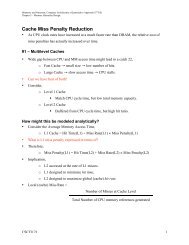
below the line segment ab. Definitions 1 and 2, as
illustrated by Figure 1, establish the initial condition
before the merge step.
Definition 1 Let {Si), 1 5 i 5 p be a partition of S
such that Vx E Sj, y E Si, j > i, the x-coordinate of
x is larger than that of y (see Figure 1).
Definition 2 Let Xi = (z1, x2,. .., x,} be an upper
hull. Then, predx, (xi) denotes xi-1 and SUCX, (xi)
denotes the point xi+l (see Figure 2).
Given two upper hulls UH(Si) and UH(Sj) where
all points in Sj are to the right of all points in Si, the
merge operations described in this paper are based on
computing for a point q E Xi the point p E Xi U
Xj which follows q in UH(Si U Sj). The following
definitions make this idea more precise (See Figure 2).
Definition 3 Let Q C s. Then, NextQ : S -+ Q as
a function such that NextQ(p) = q if and only if q is
to the right of p and is above pq’ for all q‘ E S, q’
to the rzght of p.
563

o... ........................
C
...................
line(c3
Figure 1: In this example S = {SI, S2,S3, S4) and the
points in Si that are filled in are the elements of the
upper hull of Si, namely Xi.
Definition 4 Let Y S,. Then, lm(Y) zs a function
such that lm(Y) = y* zf and only zf y- zs the leftmost
potnt tn Y such that Nextyus,,3>t(yv) @ St).
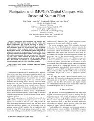
Figure 3: One step in the binary search procedure
QueryFindNext. Since the line segment .cqsue(z4)
is above the line (ezq) the algorithm will recurse on
(24.. .. , x8).
XX
hull of a point set S located in the first quadrant if and
only if all the n- 2 remaining points fall below the line
(a,b)”. We will work with a new characterization of
the upper hull of S based on the same observation,
but defined in terms of the partitioning of S given in
Definitions 1 and 4.
Consider sets S, Si and Xi as given in Definitions 1
and 2.
Definition 5 Let S’ = {e E U Xi 1 c is not dominated
by a line segment zlNeztUxj,j,i(z;),l 5 i < p},
where x; = lm(X,).
We then have the following characterization of
CH(S).
Let X represent the upper hull of a set of n points.
Let also c be a point located to the left of this
set. Below, we present a sequential algorithm called
QueryFindNext to search for q = Neztx(c). Figure
3 illustrates one step of this algorithm. This binary
search process takes time O(1og 1x1).
Procedure QueryFindNext (X,c,q)
[nput: an upper hull X = {XI,.
Zoordinate and a point c to the left of 21.
Output: a point q E X, q = NeztX(c).
1. If X = {z} then q t z and halt.
... zm} sorted by x-
2. If z,m,21suc(z,m/21) is located below the line
(c~l~,~l) then QueryFindNext((z1.. ... xlm/21},c,q).
else QueryFindNext({zr,/21,. ... zm},c,q).
3.1 Characterization of the upper hull
A classical way of characterizing the upper hull of
a point set S, as given in [14], is based on the observation
that “A line segment ab is an edge of the upper
Theorem 1 S‘ = UH(S)
0
Proof: We must consider two cases.
0 UH(S) c S’
Suppose y E UH(S), y @ SI. Then 3z such
that z:iVextxJ ,3>z(z:) dominates y. Therefore,
y $ I;H(S), which is a contradiction.
0 SI UH(S)
Suppose y E S’, y @ UH(S). Then 3p,q
withp E UH(S),q E UH(S), and q = Nezts(p) ,
such that Pq dominates y.
Therefore, both q and p cannot belong to X,
(since y E X,, meaning that y is not dominated
by any line segment with endpoints in Sz). Thus,
p and q belong respectively to X, and Xk, (j# IC).
Hence, since q = Nests(p), p E UH(S), and
q E UH(S), then 3i such that p = r:, where
z: = lm(X,). Therefore, y is dominated by a
segment x:iVextxl ,3>l(z:), which is a contradiction.
564

3.2 Parallel Merge Algorithms
In this section we describe twci parallel merge algorithms
based on the characteriza.tion of UH(S) given
in the previous section and analyze their time and
space complexity for the coarse grained model. The
following definitions and lemma are needed in the description
of the algorithms.
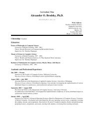
Definition 6 Let Gi
Xi and g; = Zm,(Gi). Let
Ri C Xi be composed of the points between predc, (gt)
and gt, and RF C Xi be compcsed of the points between
g: and suc~,(g:) (see Figure 4).
G,. X,. 0
S,
b
---....
Figure 4: Filled points are element of Gi which is a
subset of Xi composed of both of hollow and filled
points. Since the Rf doesn't contained any point
above the line (gfb) we have Ri = RF.
We have then the following lemma.
Lemma 1 One or both of RT cr R; is such that all
its points are under the line (gz*lVextx,,j>;(gf)).
The proof of this lemma is direct, otherwise gr $Z
Xi.
Definition 7 Let Ri denote the set R: or Ri that
has at least one point above the line
(gfNeztxj,j>i(g:)) (see Figure ,$).
Note that the size of the sets Ri is bounded by
the number of points laying between two consecutive
points in Gi.
3.3 Merge Algorithm fo.r the Case n/p 2
P2
In this section, we describe an algorithm that
merges p upper hulls, stored one per processor on a p
processor CGM, into a single upper hull using a constant
number of global communication rounds. This
algorithm requires that be greater than or equal to
p2 and thus exhibits limited scalability. This limitation
on the algorithms sca1abilit;y will be addressed in
the next section.
In order to find the upper common tangent between
an upper hull Xi and an upper hull Xi (to its right)
the algorithm computes the Next function not for the
whole set X . but for a subset of s equally spaced points
from Xi. de call this subset of equally spaced points a
splitter of Xi. This approach based on splitters greatly
reduces the amount of data that must be communicated
between processors without greatly increasing
the number of global communication rounds that are
required.
4lgorithm MergeHullsl(Xi(1 5 i 5 n),S,n,n,s,UH)
[nput: The set of 7r upper hulls Xi consisting of a total of
tt most n points from S, where Xi is stored on processor q;,
1 5 i 5 K and an integer s.
3utput: A distributed representation of the upper hull of S.
211 points on the upper hull are identified and labeled from
eft to right.
1. Each processor q; sequentially identifies a splitter set G;
composed of s evenly spaced points from Xi.
2. The processorsfind in parallelgz! = Im(G;). This is done
via a call to Procedure FindLMSubset.
3. Each processor qi computes its own RL and R;' sets
according to Definition 6, and the set R; of points which
are above the line (g1NeztG;"xj,j>;(gf)), according to
Lemma 1.
4. The processors find in parallel z: = Im(R; U gt), using
Procedure FindLMSubset. Note that by definition
Nexts(zz) @Xi.
5. Each processor qi broadcasts its zf to all q,, j > i, and
computes its own S:; according to Definition 5. By Theorem
1 this is a distributed representation of UH(S).
Analysis
Steps 2 and 4 of the algorithm above are implemented
via the procedure Fin.dLMSubset which is described
in detail the next section. The key idea in procedure
FindLMSubset is to send the elements of G; or Ri, in
Steps 2 and 4, respectively, to all larger-numbered processors
so that processors receiving G = U Gj,j < i
(at Step 2) or R = U(Rj Ug;),j < i (at Step 4) can
sequentially compute the required points using Procedure
QueryFindNext described in Section 3. The
algorithm MergeHullsl requires ST space at Step 2,
and 5 4 space at Step 4. Thus, if we set
T = s = p, then this algorithm requires n/p 2 p2
space per processor. With respect to time complexity
note that only a constant number of sort and comiiiunication
rounds are required, plus sequential computations.
The time required by the algorithm is therefore
O(? + T,(n,p)).
3.4 Merge Algorithm for the Case ri/p 1 p
In this section, we describe an algorithm, Merge-
Hulls2, that merges p upper hulls, stored one per processor
on a p processor CGM, into a single upper
hull using a constant number of global communication
rounds. Unlike the algorithm given in the previous
section this algorithm requires only n/p 2 p memory
space per processor. It is based on algorithm Merge-
Hullsl, except that; now two phases are used.
565

1. In the first phase, the algorithm MergeHullsl is
used to find the upper hull of groups of T = &
processors, with s equal to &. Kote that the
space required in this phase is O(p).
2. The second phase merges these fi upper hulls
of size at most each, instead of the p ini-
P
tial ones. Thus, with s = & again, Step 2 requires
only p space. However, we should be careful,
because the size of each set Ri is, in the worst
case, 9, implying that Step 4 requires up to LL
4
space, which is too much. Thus, a further reduction
of their sizes is needed. This is accomplished
through the simple observation that the sets R;
are upper hulls themselves, and we can recursively
apply to the Ri, for all i, the the same method
udes in MergeHullsl to find xt = Im(Ri U gf).
The algorithm is as follows. When the processors
are divided into groups, let 41 denote the z-th processor
of the i-th group.
Procedure FindLMSubset(X;, IC, w, G;,g%*)
[nput: Upper hulls Xi, 1 5 i 5 IC;, represented each in w
:onsecutively numbered processors qi, 1 5 z 5 w, and a set
T; c xi.
Output: The point gt = Im(G;). There will be a copy of gt
n each q:, 1 5 2 5 w.
1. Gather G; in processor q: , for all i.
2. Each processor ql sends its G; to all processors q:, j >
Each processor qt, for all i,z, receives
i,l 5 z 5 w.
E' = uGj,Vj < i.
3. Each processor q:, for all i,z, sequentially computes
Neztx;(g) for every g 6 E', using procedure
QueryFindNext.
4. Each processor q;, for all i, z, sends back to all processors
qi, j < i, the computed Neztx,(g), Vg E G,. Each processor
qi , for all i, receives for each g E G; the computed
Nextx, (g), Vj > i.
5. Each processor qi, for all i, computes for each g E G; the
line segment with the largest slope among gsvcc, (9) and
gNext,yi (g), j > i, finding NeztGiuxi,,>;(g). Then, it
comput,es gt? = Im(G;).
6. Broadcast g** to q5,l 5 z 5 w.
Input: Upper hulls X;,1 5 i 5 IC; represented each in w
consecutively numbered processors qi, 1 5 z 5 w, and a set
G; C Xi.
Output: The point zCf = lm(X;). There will be a copy of zCf
in each qi, 15 z 5 w.
1. FindLMSubset(X;, IC, w, G;,gt).
2. If gisucxi(gz*) is above gfNextXj,,>;(gf) then R; is
composed of all points of Xi between g: and sucG;(gf);
else R; is composed of all points of X; between
predc; (gt) and gt.
3. Let G; t R; U {gf}.
4. If IG;l *IC 5 p
then FindLMSubset(X,, IC, w, G;, zCf)
else FindLMSubHull(X;, IC, w,G;, z:)
Qlgorithm MergeHulls2(X;(l 5 i 5 r),S,n,r,s,UH)
hput: The set of r upper hulls X; consisting of a total of
tt most n points from S, where X; is stored on processor q;,
I 5 i 5 rr and an integer s.
3utput: A distributed representation of the upper hull of S.
411 points on the upper hull are identified and labeled from
eft to right.
1. Each processor 9; sequentially identifies a splitter set G;
composed of s evenly spaced points from Xi.
2. Divide the r processors into ,/% groups of fi
processors each. Do in parallel for each group:
FindLMSubHull(X; = UH(S;),IC = fi, w = l,G;,z:).
3. Each processor q; broadcasts its 51 to all qj, j > i.
4. Each processor qj computes its own Si according to Definition
5. By Theorem 1 this is a distributed representation
of the upper hull of the points in each of the fi
groups. Let r;, 1 5 i 5 fi, denote such upper hulls.
5. Each processor q; sequentially identifies a splitter set G;
composed of s evenly spaced points from r;.
6. Do in parallel: FindLMSubHull(X; = r;,k = fi,w =
J;;,G,,xf).
i. Each processor 9; broadcasts its x: to all qf, h > i and
j > 1.
8. Each processor q, computes its own Si according to Definition
5. By Theorem 1 this is a distributed representation
of UH(S).
3.5 Analysis
In the algorithm MergeHulls2, if we let T = p and
s = fi, then Step 2 requires n/p space, as seen in the
analysis of the algorithm MergeHullsl. Notice that
the space complexity of procedure FindLMSubset is
lGil * IC (at Steps 2 and 4). Thus, Step 7's call to
procedure FindLMSubset requires IGi[ * k = p space.
Now, let us analyze the space requirements of Step
7's call to procedure FindLMSubHull. At Step 1 of
FindLMSubHull, the call to procedure FindLMSubset
requires IGil*k = p space. At Step 5, IGil*k is greater
than p implying that a recursive call takes place in
566

order to reduce the size of the considered sets. Both
new calls to FindLMSubset within the recursive call
to FindLMSubHull then require p space. Therefore,
Step 7 requires nlp 2 p space, and this is the space
requirement for the MergeHulls2 algorithm as a whole.
With respect to time complexity note that only a
constant number of sort and cclmmunication rounds
are required, plus sequential computations. The time
required by the algorithm is therefore O ( F
Ts (n, P>>.
4 Triangulation of a Point Set
In this section we describe how the same ideas developed
in the previous section can be used to find
a triangulation of a planar point set. The algorithm
is based on geometric observations originally made b
Wang and Tsay and used in a PRAM algorithm [16r
We extend their basic technique in order to ensure
that the resulting algorithm is both scalable over a
large range of the ratio n/p, and uses only a constant
number of global operations rounds. Note that
the triangulation yielded by the algorithm Triangulate
presented below is not the same as the one obtained
in [16].
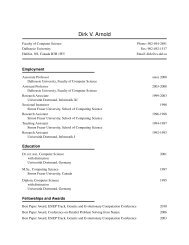
A funnel polygon consists of two x-monotone chains
and a top and a bottom line segment (see Figure 5).
Given p 2-disjoint convex hulls, Xi 15 i 5 p, and a set
of upper and lower common tangent lines the regions
between the hulls form a set of funnel polygons if the
horizontal extreme points of consecutive upper hulls
Xi are connected (see Figure 6). Funnel polygons can
easily be triangulated as will be shown in the following
algorithm. For details on funnel polygons in the
contex of triangulations, we refer the interested reader
to [16].
I’riangulate (S)
[nput: Each processor stores a set of 2 points drawn arbixarily
from S.
Output: A distributed representation of a triangulation of
S. All segment lines of the triangulation are identified and
abeled.
1. Globally sort the points in S by x-coordinate. Let S;
denote the set of sorted points now stored on processor
2.
2. Independently and in parallel, each processor i computes
the convex hull of the set S,, and the triangulation of its
convex hull. Let X ; denote the upper hull of the set Si
on processor i.
3. Label the upper funnel polygons.
4. Identify each point to its upper funnel polygon.
5. Triangulate the upper funnel polygons.
6. Repeat Steps 3-5 for the lower funnel polygons.
In Step 1 the points of S are globally sorted. Step
2 starts by connecting the horizontal extreme points
of consecutive upper hulls X; [see Figure 6). Then,
xT = lm(X;) and Neztx,,j>i(zT) are computed as
+
I
in Section 3.4. Finally, an all-to-all broadcast is performed
so that each processor i knows 23 = Zm(Xj)
and Neztx,,,>j(zj*), -for all i 2 j. Clearly, the time
complexity of this Step is dominated by the coniputation
of xi* and NezL(z*), that can be implemented
through the procedures hndLMSubset and FindLM-
SubHull described in the Section 3.4.
Steps 3 and 4 are locally performed on each processor,
using the information received at the end of
Step 2. Note that, each funnel polygon is delimited by
the segment line zfNezt(zf), and labeled Fi (see Figure
6). Given that each processor stores a table with
all common tangent lines, they can identify for each
point of their hull the funnel polygon they are part of
by a simple sequential. scan of their hull points.
Step 5 is the most technical one. Let a; and bj
denote the points in the left and right chain of a funnel
polygon, respectively (see Figure 5). Form records
containing, for all points a; on the left chain, the slope
from a point ai to its successor ai+l in the chain. Also,
form records containing, for all points b on the right
chain, the absolute value of the slope hom bj to its
successor bj+l in the chain. Note that if we sort the
a’s and b’s together by first key: funnel polygon label;
second key: slope records; third key: left chain first,
right chain next; then we get a sequence of the form
{- akak+lbhak+2bh+lbh+2bh+3bh+4pk+3 . . .). The
set of line segments tlhat forms a triangulataon of the
funnel polygon can be easily constructed by forming
the set {(b;a .) U (arbs)}, where aj is the first a to the
left of b; and b, is the first b to the left of a,.
Figure 5: Two funnel polygons.
In order to implement this step, we need only a
global sort operation on the a’s and b’s, followed by
a segmented broadcast, where each a is broadcast to
every element until the next a to its right in the sorted
list, and each b is broadcast to every element until the
next b to its righik in the sorted list. The line segments
composing the triangulation can thus be easily
constructed.
Only global sort and global communication operations
are used in addition to the call to FindLMSubset
and FindLMSubBull. Therefore, procedure Triangulation
above builds a triangulation of a point set in R2
on a CGM(n,p) in time O ( T + T,(n,p)), where
567

T,(n,p) refers to the time of a global sort of n data
on a p processor machine. Furthermore, it only requires
n/p > p local memory, and a constant number
of global communication and sort rounds.
I
Figure 6: Note that the region between the hulls
can be seen as a set of funnel polygons (U is
lm(Xl)Ne~:ts(l7n(Xl))).
5 Conclusion
In this paper we described scalable parallel algorithms
for building the Convex Hull and a Triangulation
of a planar point set for the coarse grained
multicomputer model. Our algorithms require time
O ( T + T,(n,p)), where T,(n,p) refers to the time
of a global sort of n data on a p processor machine.
Furthermore, they involve only a constant number
of global communication rounds, either running in
optimal time e(?) or in sort time ~,(n,p) for
the interconnection network in question. Our results
become optimal when Tsequ~nt'ai dominates T,(n,p),
for instance when randomized sorting algorithms are
used, or when T,(n,p) is optimal. For practical purpose
the restriction that : > p is not onerous, but for
theoretical pers ective it is interesting to note that
by performing fog(2le)l (0 < E < 1) phases (rather
than two phases) in procedure MergeHull2 this restriction
can be weakened to p 2 pE (as in [SI) while still
maintaining only a constant number of communication
rounds.
The algorithms proposed in this paper were based
on a variety of techniques arising from more theoretical
models for parallel computing, such as the PRAM
and the fine-grained hypercube. It would be interesting
to identify those parallel algorithm design techniques
for theoretical models that can be extended
to the very practical coarse graaned multzcomputer
model.
References
[l] M. J. Atallah and J.-J. Tsay. On the paralleldecomposability
of geometric problems. Proc. 5th
Annu. ACM Sympos. Comput. Geom., pages 104-
113, 1989.
[2] K.E. Batcher. Sorting networks and their applications.
Proc. AFIPS Sprmg Joznt Computer Conference,
pages 307-314, 1968.
I
[3] D. P. Bertsekas and J. N. Tsitsiklis. Parallel
and Distributed Computation,: Numerical Methods.
Prentice Hall, Englewood Cliffs, NJ, 1989.
[4] R. Cypher and C. G. Plaxton. Deterministic sorting
in nearly logarithmic time on the hypercube
and related computers. ACM Symposium on Theory
of Computing, 193-203. ACM, 1990.
[5] F. Dehne, A. Fabri and C. Kenyon Scalable and
archtecture independent parallel geometric algorithms
with high probability optimal time. Proceedings
f o the 6th IEEE SPDP, IEEE Press, 586-
593, 1994.
161 F. Dehne, A. Fabri and A. Rau-Chaplin Scalable
Parallel Geometric Algorithms for Coarse Grained
Multicomputers. AGM Symposium on Gomputational
Geometry, 1993.
[i] Deng and Gu Good algorithm design style for multiprocessors.
6th IEEE Symposium on Parallel and
Distributed Processing, 1994.
[8] M.T. Goodrich, J.J. Tsay, D.E. Vengroff, and
J.S. Vitter. External-memory computational geometry.
Foundations of Computer Science, 1993.
[9] Grand Challenges: High Performance Computing
and Communications. The FY 1992 U.S. Research
and Development Program. A Report by the Committee
on Physical, Mathematical, and Engineering
Sciences. Federal Councel for Science, Engineering,
and Technology. To Supplement the U.S.
President's Fiscal Year 1992 Budget.
[lo] R. I. Greenberg and C. E. Leiserson. Randoniized
Routing on Fat-trees. Advances in Computing
Research, 5:345-374, 1989.
[11] F.T. Leighton. Introduction to Parallel Algorithms
and Architectures: Arrays, Trees, Hypercubes.
Morgan Kaufmann Publishers, San Mateo,
CA, 1992.
[12] J.M. Marberg and E. Gafni. Sorting in constant
number of row and column phases on a mesh. Proc.
Allerton Conference on Commun,ication, Control
and Computing, 1986, pp. 603-612.
[13] R. Miller and Q. Stout. Efficent Parallel Convex
Hull Algorithms. IEEE Transcations on Computers,
37:12:1605-1618, 1988.
[14] F. P. Preparata and M. I. Shamos. Computational
Geometry: an Introduction. Springer-Verlag, New
York, NY, 1985.
[15] J. H. Reif and L. G. Valiant. A Logarithmic Time
Sort for Linear Size Networks. J. ACM, Vo1.34,
1:60-76, 1987.
[16] C. Wang and Y. Tsin. An O(1og n) Time Parallel
Algorithm for Triangulating A Set Of Points In
The Plane. Information Processing Letters, 25:55-
60, 1987.
568