Chapter 2 Review of Forces and Moments - Brown University
Chapter 2 Review of Forces and Moments - Brown University
Chapter 2 Review of Forces and Moments - Brown University

Create successful ePaper yourself
Turn your PDF publications into a flip-book with our unique Google optimized e-Paper software.
<strong>Chapter</strong> 2<br />
<strong>Review</strong> <strong>of</strong> <strong>Forces</strong> <strong>and</strong> <strong>Moments</strong><br />
2.1 <strong>Forces</strong><br />
In this chapter we review the basic concepts <strong>of</strong> forces, <strong>and</strong> force laws. Most <strong>of</strong> this material is identical<br />
to material covered in EN030, <strong>and</strong> is provided here as a review. There are a few additional sections – for<br />
example forces exerted by a damper or dashpot, an inerter, <strong>and</strong> interatomic forces are discussed in<br />
Section 2.1.7.<br />
2.1.1 Definition <strong>of</strong> a force<br />
Engineering design calculations nearly always use classical (Newtonian) mechanics. In classical<br />
mechanics, the concept <strong>of</strong> a `force’ is based on experimental observations that everything in the universe<br />
seems to have a preferred configuration – masses appear to attract each other; objects with opposite<br />
charges attract one another; magnets can repel or attract one another; you are probably repelled by your<br />
pr<strong>of</strong>essor. But we don’t really know why this is (except perhaps the last one).<br />
The idea <strong>of</strong> a force is introduced to quantify the tendency <strong>of</strong> objects to move towards their preferred<br />
configuration. If objects accelerate very quickly towards their preferred configuration, then we say that<br />
there’s a big force acting on them. If they don’t move (or move at constant velocity), then there is no<br />
force. We can’t see a force; we can only deduce its existence by observing its effect.<br />
Specifically, forces are defined through Newton’s laws <strong>of</strong> motion<br />
0. A `particle’ is a small mass at some position in space.<br />
1. When the sum <strong>of</strong> the forces acting on a particle is zero, its velocity is<br />
constant;<br />
2. The sum <strong>of</strong> forces acting on a particle <strong>of</strong> constant mass is equal to the<br />
product <strong>of</strong> the mass <strong>of</strong> the particle <strong>and</strong> its acceleration;<br />
3. The forces exerted by two particles on each other are equal in magnitude<br />
<strong>and</strong> opposite in direction.<br />
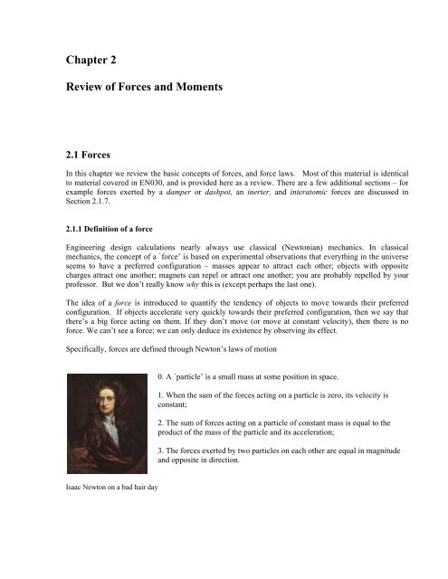
Isaac Newton on a bad hair day
The second law provides the definition <strong>of</strong> a force – if a mass m has acceleration a, the force F acting on it<br />
is<br />
F = ma<br />
Of course, there is a big problem with Newton’s laws – what do we take as a fixed point (<strong>and</strong> orientation)<br />
in order to define acceleration? The general theory <strong>of</strong> relativity addresses this issue rigorously. But for<br />
engineering calculations we can usually take the earth to be fixed, <strong>and</strong> happily apply Newton’s laws. In<br />
rare cases where the earth’s motion is important, we take the stars far from the solar system to be fixed.<br />
2.1.2 Causes <strong>of</strong> force<br />
<strong>Forces</strong> may arise from a number <strong>of</strong> different effects, including<br />
(i) Gravity;<br />
(ii) Electromagnetism or electrostatics;<br />
(iii) Pressure exerted by fluid or gas on part <strong>of</strong> a structure<br />
(v) Wind or fluid induced drag or lift forces;<br />
(vi) Contact forces, which act wherever a structure or component touches anything;<br />
(vii) Friction forces, which also act at contacts.<br />
Some <strong>of</strong> these forces can be described by universal laws. For example, gravity forces can be calculated<br />
using Newton’s law <strong>of</strong> gravitation; electrostatic forces acting between charged particles are governed by<br />
Coulomb’s law; electromagnetic forces acting between current carrying wires are governed by Ampere’s<br />
law; buoyancy forces are governed by laws describing hydrostatic forces in fluids. Some <strong>of</strong> these<br />
universal force laws are listed in Section 2.6.<br />
Some forces have to be measured. For example, to determine friction forces acting in a machine, you may<br />
need to measure the coefficient <strong>of</strong> friction for the contacting surfaces. Similarly, to determine<br />
aerodynamic lift or drag forces acting on a structure, you would probably need to measure its lift <strong>and</strong> drag<br />
coefficient experimentally. Lift <strong>and</strong> drag forces are described in Section 2.6. Friction forces are<br />
discussed in Section 12.<br />
Contact forces are pressures that act on the small area <strong>of</strong> contact between two objects. Contact forces can<br />
either be measured, or they can be calculated by analyzing forces <strong>and</strong> deformation in the system <strong>of</strong><br />
interest. Contact forces are very complicated, <strong>and</strong> are discussed in more detail in Section 8.<br />
2.1.3 Units <strong>of</strong> force <strong>and</strong> typical magnitudes<br />
In SI units, the st<strong>and</strong>ard unit <strong>of</strong> force is the Newton, given the symbol N.<br />
The Newton is a derived unit, defined through Newton’s second law <strong>of</strong> motion – a force <strong>of</strong> 1N causes a 1<br />
2<br />
kg mass to accelerate at 1 ms − .<br />
The fundamental unit <strong>of</strong> force in the SI convention is kg m/s 2<br />
In US units, the st<strong>and</strong>ard unit <strong>of</strong> force is the pound, given the symbol lb or lbf (the latter is an abbreviation<br />
for pound force, to distinguish it from pounds weight)<br />
A force <strong>of</strong> 1 lbf causes a mass <strong>of</strong> 1 slug to accelerate at 1 ft/s 2
US units have a frightfully confusing way <strong>of</strong> representing mass – <strong>of</strong>ten the mass <strong>of</strong> an object is reported<br />
as weight, in lb or lbm (the latter is an abbreviation for pound mass). The weight <strong>of</strong> an object in lb is not<br />
mass at all – it’s actually the gravitational force acting on the mass. Therefore, the mass <strong>of</strong> an object in<br />
slugs must be computed from its weight in pounds using the formula<br />
W (lb)<br />
m(slugs)<br />
=<br />
2<br />
g(ft/s )<br />
where g=32.1740 ft/s 2 is the acceleration due to gravity.<br />
A force <strong>of</strong> 1 lb(f) causes a mass <strong>of</strong> 1 lb(m) to accelerate at 32.1740 ft/s 2<br />
The conversion factors from lb to N are<br />
1 lb = 4.448 N<br />
1 N = 0.2248 lb<br />
(www.onlineconversion.com is a h<strong>and</strong>y resource, as long as you can tolerate all the hideous<br />
advertisements…)<br />
As a rough guide, a force <strong>of</strong> 1N is about equal to the weight <strong>of</strong> a medium sized apple. A few typical force<br />
magnitudes (from `The Sizesaurus’, by Stephen Strauss, Avon Books, NY, 1997) are listed in the table<br />
below<br />
Force Newtons Pounds Force<br />
Gravitational Pull <strong>of</strong> the Sun on Earth 22<br />
3.5×<br />
10<br />
21<br />
7.9×<br />
10<br />
Gravitational Pull <strong>of</strong> the Earth on the Moon 20<br />
2×<br />
10<br />
19<br />
4.5×<br />
10<br />
Thrust <strong>of</strong> a Saturn V rocket engine 7<br />
3.3×<br />
10<br />
6<br />
7.4×<br />
10<br />
Thrust <strong>of</strong> a large jet engine 5<br />
7.7×<br />
10<br />
5<br />
1.7×<br />
10<br />
Pull <strong>of</strong> a large locomotive 5<br />
5×<br />
10<br />
5<br />
1.1×<br />
10<br />
Force between two protons in a nucleus 4<br />
10<br />
3<br />
10<br />
Gravitational pull <strong>of</strong> the earth on a person 2<br />
7.3×<br />
10<br />
2<br />
1.6×<br />
10<br />
Maximum force exerted upwards by a forearm 2<br />
2.7× 10 60<br />
Gravitational pull <strong>of</strong> the earth on a 5 cent coin 2<br />
5.1×<br />
10 − 1.1×<br />
10 −2<br />
Force between an electron <strong>and</strong> the nucleus <strong>of</strong> a Hydrogen atom 6<br />
8×<br />
10 − 1.8×<br />
10 −8
2.1.4 Classification <strong>of</strong> forces: External forces, constraint forces <strong>and</strong> internal forces.<br />
When analyzing forces in a structure or machine, it is conventional to classify forces as external forces;<br />
constraint forces or internal forces.<br />
External forces arise from interaction between the system <strong>of</strong> interest <strong>and</strong> its surroundings.<br />
Examples <strong>of</strong> external forces include gravitational forces; lift or drag forces arising from wind loading;<br />
electrostatic <strong>and</strong> electromagnetic forces; <strong>and</strong> buoyancy forces; among others. Force laws governing these<br />
effects are listed later in this section.<br />
Constraint forces are exerted by one part <strong>of</strong> a structure on another, through joints, connections or contacts<br />
between components. Constraint forces are very complex, <strong>and</strong> will be discussed in detail in Section 8.<br />
Internal forces are forces that act inside a solid part <strong>of</strong> a structure or component. For example, a stretched<br />
rope has a tension force acting inside it, holding the rope together. Most solid objects contain very<br />
complex distributions <strong>of</strong> internal force. These internal forces ultimately lead to structural failure, <strong>and</strong> also<br />
cause the structure to deform. The purpose <strong>of</strong> calculating forces in a structure or component is usually to<br />
deduce the internal forces, so as to be able to design stiff, lightweight <strong>and</strong> strong components. We will<br />
not, unfortunately, be able to develop a full theory <strong>of</strong> internal forces in this course – a proper discussion<br />
requires underst<strong>and</strong>ing <strong>of</strong> partial differential equations, as well as vector <strong>and</strong> tensor calculus. However, a<br />
brief discussion <strong>of</strong> internal forces in slender members will be provided in Section 9.<br />
2.1.5 Mathematical representation <strong>of</strong> a force.<br />
Force is a vector – it has a magnitude (specified in Newtons, or lbf, or<br />
whatever), <strong>and</strong> a direction.<br />
A force is therefore always expressed mathematically as a vector<br />
F<br />
quantity. To do so, we follow the usual rules, which are described in<br />
z x<br />
O<br />
y<br />
more detail in the vector tutorial. The procedure is<br />
x<br />
1. Choose basis vectors { i, j, k } or { e1, e2, e<br />
2}<br />
that establish three<br />
fixed (<strong>and</strong> usually perpendicular) directions in space;<br />
i<br />
2. Using geometry or trigonometry, calculate the force component along each <strong>of</strong> the three reference<br />
directions ( Fx , Fy, F<br />
z)<br />
or ( F1, F2, F<br />
3)<br />
;<br />
3. The vector force is then reported as<br />
F= Fxi+ Fyj+ Fzk = F1e1+ F2e2+<br />
F3e<br />
3<br />
(appropriate units)<br />
For calculations, you will also need to specify the point where the force acts on your system or structure.<br />
To do this, you need to report the position vector <strong>of</strong> the point where the force acts on the structure.<br />
The procedure for representing a position vector is also described in detail in the vector tutorial. To do so,<br />
you need to:<br />
1. Choose an origin<br />
2. Choose basis vectors { i, j, k } or { e1, e2, e<br />
2}<br />
that establish three fixed directions in space (usually<br />
we use the same basis for both force <strong>and</strong> position vectors)<br />
k<br />
j<br />
F z<br />
F y
3. Specify the distance you need to travel along each direction to get from the origin to the point <strong>of</strong><br />
application <strong>of</strong> the force ( rx , ry, r<br />
z)<br />
or ( r1, r2, r<br />
3)<br />
4. The position vector is then reported as<br />
r = rxi+ ryj+ rzk = r1e1+ r2e2+<br />
r3e<br />
3<br />
(appropriate units)<br />
2.1.6 Measuring forces<br />
Engineers <strong>of</strong>ten need to measure forces. According to the definition, if we want to measure a<br />
force, we need to get hold <strong>of</strong> a 1 kg mass, have the force act on it somehow, <strong>and</strong> then measure<br />
the acceleration <strong>of</strong> the mass. The magnitude <strong>of</strong> the acceleration tells us the magnitude <strong>of</strong> the<br />
force; the direction <strong>of</strong> motion <strong>of</strong> the mass tells us the direction <strong>of</strong> the force. Fortunately, there<br />
are easier ways to measure forces.<br />
In addition to causing acceleration, forces cause objects to deform – for example, a force will<br />
stretch or compress a spring; or bend a beam. The deformation can be measured, <strong>and</strong> the force<br />
can be deduced.<br />
The simplest application <strong>of</strong> this phenomenon is a spring scale. The change in length <strong>of</strong> a spring is<br />
proportional to the magnitude <strong>of</strong> the force causing it to stretch (so long as the force is not too large!)– this<br />
relationship is known as Hooke’s law <strong>and</strong> can be expressed as an equation<br />
kδ = F<br />
where the spring stiffness k depends on the material the spring is made from, <strong>and</strong> the shape <strong>of</strong> the spring.<br />
The spring stiffness can be measured experimentally to calibrate the spring.<br />
Spring scales are not exactly precision instruments, <strong>of</strong> course. But the same principle is used in more<br />
sophisticated instruments too. <strong>Forces</strong> can be measured precisely using a `force transducer’ or `load cell’<br />
(A search for `force transducer’ on any search engine will bring up a huge variety <strong>of</strong> these – a few are<br />
shown in the picture). The simplest load cell works much like a spring scale – you can load it in one<br />
direction, <strong>and</strong> it will provide an electrical signal proportional to the magnitude <strong>of</strong> the force. Sophisticated<br />
load cells can measure a force vector, <strong>and</strong> will record all three force components. Really fancy load cells<br />
measure both force vectors, <strong>and</strong> torque or moment vectors.<br />
Simple force transducers capable <strong>of</strong> measuring a single force component. The instrument on the right is<br />
called a `proving ring’ – there’s a short article describing how it works at<br />
http://www.mel.nist.gov/div822/proving_ring.htm
A sophisticated force transducer produced by MTS systems, which is capable <strong>of</strong> measuring forces <strong>and</strong><br />
moments acting on a car’s wheel in-situ. The spec for this device can be downloaded at<br />
www.mts.com/downloads/SWIF2002_100-023-513.pdf.pdf<br />
The basic design <strong>of</strong> all these load cells is the same – they measure (very precisely) the deformation in a<br />
part <strong>of</strong> the cell that acts like a very stiff spring. One example (from<br />
http://www.s<strong>and</strong>ia.gov/isrc/Load_Cell/load_cell.html ) is shown on the<br />
right. In this case the `spring’ is actually a tubular piece <strong>of</strong> high-strength<br />
steel. When a force acts on the cylinder, its length decreases slightly. The<br />
deformation is detected using `strain gages’ attached to the cylinder. A<br />
strain gage is really just a thin piece <strong>of</strong> wire, which deforms with the<br />
cylinder. When the wire gets shorter, its electrical resistance decreases –<br />
this resistance change can be measured, <strong>and</strong> can be used to work out the<br />
force. It is possible to derive a formula relating the force to the change in<br />
resistance, the load cell geometry, <strong>and</strong> the material properties <strong>of</strong> steel, but<br />
the calculations involved are well beyond the scope <strong>of</strong> this course.<br />
The most sensitive load cell currently available is the atomic force<br />
microscope (AFM) – which as the name suggests, is<br />
intended to measure forces between small numbers<br />
<strong>of</strong> atoms. This device consists <strong>of</strong> a very thin (about<br />
1 μ m ) cantilever beam, clamped at one end, with a<br />
sharp tip mounted at the other. When the tip is<br />
brought near a sample, atomic interactions exert a<br />
force on the tip <strong>and</strong> cause the cantilever to bend.<br />
The bending is detected by a laser-mirror system.<br />
The device is capable <strong>of</strong> measuring forces <strong>of</strong> about<br />
12<br />
1 pN (that’s10 − N!!), <strong>and</strong> is used to explore the<br />
properties <strong>of</strong> surfaces, <strong>and</strong> biological materials such<br />
as DNA str<strong>and</strong>s <strong>and</strong> cell membranes. A nice article<br />
on the AFM can be found at http://www.di.com
Selecting a load cell<br />
As an engineer, you may need to purchase a load cell to measure a force. Here are a few considerations<br />
that will guide your purchase.<br />
1. How many force (<strong>and</strong> maybe moment) components do you need to measure? Instruments that<br />
measure several force components are more expensive…<br />
2. Load capacity – what is the maximum force you need to measure?<br />
3. Load range – what is the minimum force you need to measure?<br />
4. Accuracy<br />
5. Temperature stability – how much will the reading on the cell change if the temperature changes?<br />
6. Creep stability – if a load is applied to the cell for a long time, does the reading drift?<br />
7. Frequency response – how rapidly will the cell respond to time varying loads? What is the<br />
maximum frequency <strong>of</strong> loading that can be measured?<br />
8. Reliability<br />
9. Cost<br />
2.1.7 Force Laws<br />
In this section, we list equations that can be used to calculate forces associated with<br />
(i) Gravity<br />
(ii) <strong>Forces</strong> exerted by linear springs<br />
(iii) Electrostatic forces<br />
(iv) Electromagnetic forces<br />
(v) Hydrostatic forces <strong>and</strong> buoyancy<br />
(vi) Aero- <strong>and</strong> hydro-dynamic lift <strong>and</strong> drag forces<br />
Gravitation<br />
Gravity forces acting on masses that are a large distance apart<br />
Consider two masses m<br />
1<br />
<strong>and</strong> m<br />
2<br />
that are a distance d<br />
e m 2<br />
12<br />
apart. Newton’s law <strong>of</strong> gravitation states that mass<br />
m1<br />
will experience a force<br />
m<br />
F<br />
1<br />
d<br />
Gm1m<br />
2<br />
F=<br />
e<br />
2 12<br />
d<br />
where e<br />
12<br />
is a unit vector pointing from mass m<br />
1<br />
to mass m<br />
2<br />
, <strong>and</strong> G is the Gravitation constant. Mass<br />
m<br />
2<br />
will experience a force <strong>of</strong> equal magnitude, acting in the opposite direction.<br />
In SI units,<br />
G = 6.673×<br />
10 m kg s<br />
−11 3 -1 -2<br />
The law is strictly only valid if the masses are very small (infinitely small, in fact) compared with d – so<br />
the formula works best for calculating the force exerted by one planet or another; or the force exerted by<br />
the earth on a satellite.
Gravity forces acting on a small object close to the<br />
earth’s surface<br />
For engineering purposes, we can usually assume<br />
that<br />
1. The earth is spherical, with a radius R<br />
2. The object <strong>of</strong> interest is small compared<br />
with R<br />
3. The object’s height h above the earths<br />
surface is small compared to R<br />
If the first two assumptions are valid, then one can<br />
show that Newton’s law <strong>of</strong> gravitation implies that a<br />
mass m at a height h above the earth’s surface experiences a force<br />
GMm<br />
F=−<br />
e<br />
2 r<br />
( R+<br />
h)<br />
where M is the mass <strong>of</strong> the earth; m is the mass <strong>of</strong> the object; R is the earth’s radius, G is the gravitation<br />
constant <strong>and</strong> e<br />
r<br />
is a unit vector pointing from the center <strong>of</strong> the earth to the mass m. (Why do we have to<br />
show this? Well, the mass m actually experiences a force <strong>of</strong> attraction towards every point inside the<br />
earth. One might guess that points close to the earth’s surface under the mass would attract the mass<br />
more than those far away, so the earth would exert a larger gravitational force than a very small object<br />
with the same mass located at the earth’s center. But this turns out not to be the case, as long as the earth<br />
is perfectly uniform <strong>and</strong> spherical).<br />
If the third assumption (h
TABLE OF POSITIONS OF CENTER OF MASS FOR COMMON OBJECTS<br />
Rectangular prism Circular cylinder Half-cylinder<br />
Solid hemisphere Thin hemispherical shell Cone<br />
Triangular Prism<br />
Thin triangular laminate<br />
Some subtleties about gravitational interactions<br />
There are some situations where the simple equations in the preceding section don’t work. Surveyors<br />
know perfectly well that the earth is no-where near spherical; its density is also not uniform. The earth’s<br />
gravitational field can be quite severely distorted near large mountains, for example. So using the simple<br />
gravitational formulas in surveying applications (e.g. to find the `vertical’ direction) can lead to large<br />
errors.<br />
Also, the center <strong>of</strong> gravity <strong>of</strong> an object is not the same as its center <strong>of</strong> mass. Gravity is actually a<br />
distributed force. When two nearby objects exert a gravitational force on each other, every point in one<br />
body is attracted towards every point inside its neighbor. The distributed force can be replaced by a<br />
single, statically equivalent force, but the point where the equivalent force acts depends on the relative<br />
positions <strong>of</strong> the two objects, <strong>and</strong> is not generally a fixed point in either solid. One consequence <strong>of</strong> this<br />
behavior is that gravity can cause rotational accelerations, as well as linear accelerations. For example,<br />
the resultant force <strong>of</strong> gravity exerted on the earth by the sun <strong>and</strong> moon does not act at the center <strong>of</strong> mass<br />
<strong>of</strong> the earth. As a result, the earth precesses – that is to say, its axis <strong>of</strong> rotation changes with time.
<strong>Forces</strong> exerted by springs<br />
A solid object (e.g. a rubber b<strong>and</strong>) can be made to exert forces by stretching it. The forces exerted by a<br />
solid that is subjected to a given deformation depend on the shape <strong>of</strong> the component, the materials it is<br />
made from, <strong>and</strong> how it is connected to its surroundings. Solid objects can also exert moments, or torques<br />
– we will define these shortly. <strong>Forces</strong> exerted by solid components in a machine or structure are<br />
complicated, <strong>and</strong> will be discussed in detail separately. Here, we restrict attention to the simplest case:<br />
forces exerted by linear springs.<br />
A spring scale is a good example <strong>of</strong> a linear spring. You can attach it<br />
to something at both ends. If you stretch or compress the spring, it<br />
will exert forces on whatever you connected to.<br />
The forces exerted by the ends <strong>of</strong> the spring always act along the line<br />
<strong>of</strong> the spring. The magnitude <strong>of</strong> the force is (so long as you don’t<br />
stretch the spring too much) given by the formula<br />
F = k( L−<br />
a)<br />
where a is the un-stretched spring length; L is the stretched length,<br />
<strong>and</strong> k is the spring stiffness.<br />
In the SI system, k has units <strong>of</strong> N/m.<br />
Note that when you draw a picture showing the forces exerted by a<br />
spring, you must always assume that the spring is stretched, so that<br />
the forces exerted by the spring are attractive. If you don’t do this,<br />
your sign convention will be inconsistent with the formula<br />
F = k( L− a)<br />
, which assumes that a compressed spring (L
where L is the length, <strong>and</strong> η is the rate constant <strong>of</strong> the dashpot. Air filled dashpots are somewhat more<br />
complicated, because the compressibility <strong>of</strong> the air makes them behave like a combination <strong>of</strong> a dashpot<br />
<strong>and</strong> spring connected end-to-end.<br />
In the SI system, η has units <strong>of</strong> Ns/m.<br />
Note that when you draw a picture showing the forces exerted by a dashpot, you must always assume that<br />
the length <strong>of</strong> the dashpot is increasing, so that the forces exerted by the ends <strong>of</strong> the dashpot are attractive.<br />
<strong>Forces</strong> exerted by an ‘Inerter’<br />
The ‘Inerter’ is a device that exerts forces proportional to the relative<br />
acceleration <strong>of</strong> its two ends. It was invented in 1997 <strong>and</strong> used in secret by<br />
the McLaren Formula 1 racing team to improve the performance <strong>of</strong> their<br />
cars, but in 2008 was made broadly available<br />
(http://www.admin.cam.ac.uk/news/dp/2008081906)<br />
F<br />
F<br />
The device is so simple that it is difficult to believe that it has taken over 100<br />
years <strong>of</strong> vehicle design to think <strong>of</strong> it – but the secret is really in how to use<br />
the device to design suspensions than in the device itself. The device works<br />
by spinning a flywheel between two moving rods, as sketched in the figure.<br />
The forces exerted by the ends <strong>of</strong> the inerter always act along the line <strong>of</strong> the<br />
inerter. The magnitude <strong>of</strong> the force exerted by an inerter is given by the formula<br />
2<br />
d L<br />
F = μ<br />
2<br />
dt<br />
where L is the length, <strong>and</strong> μ is the inertia constant <strong>of</strong> the dashpot.<br />
F<br />
<strong>Forces</strong> exerted<br />
by inerter<br />
F<br />
<strong>Forces</strong> acting<br />
on inerter<br />
In the SI system, μ has units <strong>of</strong> Ns 2 /m.<br />
Electrostatic forces<br />
As an engineer, you will need to be able to design structures <strong>and</strong> machines that manage forces.<br />
Controlling gravity is, alas, beyond the capabilities <strong>of</strong> today’s engineers. It’s also difficult (but not<br />
impossible) to design a spring with a variable stiffness or unstretched length. But there are forces that<br />
you can easily control. Electrostatic <strong>and</strong> electromagnetic forces are among the most important ones.<br />
Electrostatic forces are exerted on, <strong>and</strong> by, charged objects. The concepts <strong>of</strong> electrical potential, current<br />
<strong>and</strong> charge are based on experiments. A detailed discussion <strong>of</strong> these topics is beyond the scope <strong>of</strong> this<br />
course (it will be covered in detail in EN51), but electromagnetic <strong>and</strong> electrostatic forces are so important<br />
in the design <strong>of</strong> engines <strong>and</strong> machines that the main rules governing forces in these systems will be<br />
summarized here.
Electrostatic forces acting on two small charged objects that are a large distance apart<br />
Coulomb’s Law states that if like charges Q<br />
1<br />
<strong>and</strong> Q<br />
2<br />
are induced on two particles that are a distance d<br />
apart, then particle 1 will experience a force<br />
QQ<br />
1 2<br />
F=−<br />
e<br />
2 12<br />
4πε d<br />
(acting away from particle 2), where ε is a<br />
fundamental physical constant known as the<br />
Permittivity <strong>of</strong> the medium surrounding the particles<br />
(like the Gravitational constant, its value must be<br />
determined by experiment).<br />
F<br />
+Q 1<br />
e 12<br />
d<br />
+Q 2<br />
In SI units, Q1,<br />
Q<br />
2<br />
are specified in Coulombs, d is in meters, <strong>and</strong> ε is the permittivity <strong>of</strong> free space, with<br />
2 -1 -3<br />
fundamental units Amperes kg m . Permittivity is more usually specified using derived units, in<br />
Farads per meter. The Farad is the unit <strong>of</strong> capacitance.<br />
The value <strong>of</strong> ε for air is very close to that <strong>of</strong> a vacuum. The permittivity <strong>of</strong> a vacuum is denoted by ε<br />
0<br />
.<br />
-12 -1<br />
In SI units its value is approximately 8.854185 × 10 Fm<br />
Like gravitational forces, the electrostatic forces acting on 3D objects with a general distribution <strong>of</strong><br />
charge must be determined using complicated calculations. It’s worth giving results for two cases that<br />
arise frequently in engineering designs:<br />
<strong>Forces</strong> acting between charged flat parallel plates<br />
F<br />
Two parallel plates, which have equal <strong>and</strong> opposite charges Q <strong>and</strong><br />
are separated by a distance d , experience an attractive force with<br />
magnitude<br />
F = Q 2 /(2 ε )<br />
The force can be thought <strong>of</strong> as acting at the center <strong>of</strong> gravity <strong>of</strong> the<br />
plates.<br />
+Q<br />
Q<br />
F<br />
d<br />
Two parallel plates, which have area A, are separated by a distance d, <strong>and</strong> are connected to a powersupply<br />
that imposes an electrical potential difference V<br />
across the plates, experience an attractive force with<br />
F<br />
magnitude<br />
2 2<br />
+V Area A<br />
F = AV ε /(2 d )<br />
+<br />
d<br />
The force can be thought <strong>of</strong> as acting at the center <strong>of</strong><br />
V<br />
- V<br />
gravity <strong>of</strong> the plates.<br />
Area A<br />
F
Applications <strong>of</strong> electrostatic forces:<br />
Electrostatic forces are small, <strong>and</strong> don’t have many applications in conventional mechanical systems.<br />
However, they are <strong>of</strong>ten used to construct tiny motors for micro-electro-mechanical systems (MEMS).<br />
The basic idea is to construct a parallel-plate capacitor, <strong>and</strong> then to apply force to the machine by<br />
connecting the plates to a power-supply. The pictures below show examples <strong>of</strong> comb drive motors.<br />
An experimental comb drive MEMS<br />
actuator developed at S<strong>and</strong>ia National<br />
Labs,<br />
http://mems.s<strong>and</strong>ia.gov/scripts/index.asp<br />
A rotary comb drive actuator developed at iolon inc.<br />
Its purpose is to rotate the mirror at the center, which<br />
acts as an optical switch.<br />
The configurations used in practice are basically large numbers <strong>of</strong> parallel plate capacitors. A detailed<br />
discussion <strong>of</strong> forces in these systems will be deferred to future courses.<br />
Electrostatic forces are also exploited in the design <strong>of</strong> oscilloscopes, television monitors, <strong>and</strong> electron<br />
microscopes. These systems generate charged particles (electrons), for example by heating a tungsten<br />
wire. The electrons are emitted into a strong electrostatic field, <strong>and</strong> so are subjected to a large force. The<br />
force then causes the particles to accelerate – but we can’t talk about accelerations in this course so you’ll<br />
have to take EN4 to find out what happens next…<br />
Electromagnetic forces<br />
Electromagnetic forces are exploited more widely than electrostatic<br />
forces, in the design <strong>of</strong> electric motors, generators, <strong>and</strong> electromagnets.<br />
Ampere’s Law states that two long parallel wires which have length L,<br />
carry electric currents I<br />
1<br />
<strong>and</strong> I<br />
2<br />
, <strong>and</strong> are a small distance d apart, will<br />
experience an attractive force with magnitude<br />
F = μ0I1I2 L/(2 π d)<br />
where μ<br />
0<br />
is a constant known as the permeability <strong>of</strong> free space.<br />
I 1 d I 2<br />
+<br />
+<br />
V<br />
F F<br />
- V 1 2<br />
L<br />
2 -1 -2<br />
In SI units, μ<br />
0<br />
has fundamental units <strong>of</strong> kg m sec A , but is usually<br />
specified in derived units <strong>of</strong> Henry per meter. The Henry is the unit <strong>of</strong> inductance.
The value <strong>of</strong> μ0<br />
is exactly<br />
4π<br />
10<br />
−7<br />
× H/m<br />
Electromagnetic forces between more generally shaped current carrying wires <strong>and</strong> magnets are governed<br />
by a complex set <strong>of</strong> equations. A full discussion <strong>of</strong> these physical laws is beyond the scope <strong>of</strong> this course,<br />
<strong>and</strong> will be covered in EN51.<br />
Applications <strong>of</strong> electromagnetic forces<br />
Electromagnetic forces are widely exploited in the design <strong>of</strong> electric motors; force actuators; solenoids;<br />
<strong>and</strong> electromagnets. All these applications are based upon the principle that a current-carrying wire in a<br />
magnetic field is subject to a force. The magnetic field can either be induced by a permanent magnet (as<br />
in a DC motor); or can be induced by passing a current through a second wire (used in some DC motors,<br />
<strong>and</strong> all AC motors). The general trends <strong>of</strong> forces in electric motors follow Ampere’s law: the force<br />
exerted by the motor increases linearly with electric current in the armature; increases roughly in<br />
proportion to the length <strong>of</strong> wire used to wind the armature, <strong>and</strong> depends on the geometry <strong>of</strong> the motor.<br />
Two examples <strong>of</strong> DC motors – the picture on the right is cut open to show the windings. You can find<br />
more information on motors at http://my.execpc.com/~rhoadley/magmotor.htm<br />
Hydrostatic <strong>and</strong> buoyancy forces<br />
When an object is immersed in a stationary fluid, its surface<br />
is subjected to a pressure. The pressure is actually induced<br />
in the fluid by gravity: the pressure at any depth is<br />
HMS Bounty<br />
p<br />
effectively supporting the weight <strong>of</strong> fluid above that depth.<br />
a<br />
d<br />
A pressure is a distributed force. If a pressure p acts on a<br />
surface, a small piece <strong>of</strong> the surface with area dA is<br />
subjected to a force<br />
dF=−p dA n<br />
p = p a<br />
+ ρgd<br />
where n is a unit vector perpendicular to the surface. The total force on a surface must be calculated by<br />
integration. We will show how this is done shortly.<br />
The pressure in a stationary fluid varies linearly with depth below the fluid surface<br />
p = pa<br />
+ ρ gd<br />
where p<br />
a<br />
is atmospheric pressure (<strong>of</strong>ten neglected as it’s generally small compared with the second<br />
term); ρ is the fluid density; g is the acceleration due to gravity; <strong>and</strong> d is depth below the fluid surface.
Archimedes’ principle gives a simple way to calculate the resultant force exerted by fluid pressure on an<br />
immersed object.<br />
The magnitude <strong>of</strong> the resultant force is equal to<br />
the weight <strong>of</strong> water displaced by the object. The<br />
direction is perpendicular to the fluid surface.<br />
Thus, if the fluid has mass density ρ , <strong>and</strong> a<br />
volume V<br />
I<br />
<strong>of</strong> the object lies below the surface<br />
<strong>of</strong> the fluid, the resultant force due to fluid<br />
pressure is<br />
F<br />
Center <strong>of</strong> mass <strong>of</strong><br />
submerged portion V I<br />
= ρgV I<br />
j<br />
F<br />
Volume V I lies below<br />
fluid surface<br />
The force acts at the center <strong>of</strong> buoyancy <strong>of</strong> the immersed object. The center <strong>of</strong> buoyancy can be<br />
calculated by finding the center <strong>of</strong> mass <strong>of</strong> the displaced fluid (i.e. the center <strong>of</strong> mass <strong>of</strong> the portion <strong>of</strong> the<br />
immersed object that lies below the fluid surface).<br />
The buoyancy force acts in addition to gravity loading. If the object floats, the gravitational force is equal<br />
<strong>and</strong> opposite to the buoyancy force. The force <strong>of</strong> gravity acts (as usual) at the center <strong>of</strong> mass <strong>of</strong> the entire<br />
object.<br />
Aerodynamic lift <strong>and</strong> drag forces<br />
Engineers who design large<br />
bridges, buildings, or fast-moving<br />
terrestrial vehicles, spend much<br />
time <strong>and</strong> effort in managing aeroor<br />
hydro-dynamic forces.<br />
Hydrodynamic forces are also <strong>of</strong><br />
great interest to engineers who<br />
design bearings <strong>and</strong> car tires, since<br />
hydrodynamic forces can cause one<br />
surface to float above another, so<br />
reducing friction to very low<br />
levels.<br />
V<br />
F L<br />
(Lift acts perpendicular<br />
to flow)<br />
F D<br />
Flow is asymmetric near airfoil<br />
(Drag acts parallel<br />
to flow)<br />
In general, when air or fluid flow past an object (or equivalently, if the object moves through stationary<br />
fluid or gas), the object is subjected to two forces:<br />
1. A Drag force, which acts parallel to the direction <strong>of</strong> air or fluid flow<br />
2. A Lift force, which acts perpendicular to the direction <strong>of</strong> air or fluid flow.<br />
The forces act at a point known as the center <strong>of</strong> lift <strong>of</strong> the object – but there’s no simple way to predict<br />
where this point is.<br />
The lift force is present only if airflow past the object is unsymmetrical (i.e. faster above or below the<br />
object). This asymmetry can result from the shape <strong>of</strong> the object itself (this effect is exploited in the
design <strong>of</strong> airplane wings); or because the object is spinning (this effect is exploited by people who throw,<br />
kick, or hit balls for a living).<br />
Two effects contribute to drag:<br />
(1) Friction between the object’s surface <strong>and</strong> the fluid or air. The friction force depends on the<br />
object’s shape <strong>and</strong> size; on the speed <strong>of</strong> the flow; <strong>and</strong> on the viscosity <strong>of</strong> the fluid, which is a<br />
measure <strong>of</strong> the shear resistance <strong>of</strong> the fluid. Air has a low viscosity; ketchup has a high<br />
viscosity. Viscosity is <strong>of</strong>ten given the symbol η , <strong>and</strong> has the rather strange units in the SI<br />
2<br />
system <strong>of</strong> Nsm − . In `American’ units viscosity has units <strong>of</strong> `Poise’ (or sometimes<br />
2<br />
centipoises – that’s 10 − 2<br />
Poise). The conversion factor is 1P= 0.1Nsm − . (Just to be<br />
confusing, there’s another measure <strong>of</strong> viscosity, called kinematic viscosity, or specific<br />
viscosity, which is ς = η/<br />
ρ , where ρ is the mass density <strong>of</strong> the material. In this course<br />
we’ll avoid using kinematic viscosity, but you should be aware that it exists!) Typical<br />
−5 −2<br />
numbers are: Air: η ≈ 1.73× 10 Nsm for a st<strong>and</strong>ard atmosphere (see<br />
http://users.wpi.edu/~ierardi/PDF/air_nu_plot.PDF for a more accurate number) ; Water,<br />
−2<br />
−2<br />
−2<br />
η ≈ 0.001Nsm ; SAE40 motor oil η ≈ 0.5Nsm , ketchup η ≈ 60Nsm (It’s hard to<br />
give a value for the viscosity <strong>of</strong> ketchup, because it’s thixotropic. See if you can find out<br />
what this cool word means – it’s a h<strong>and</strong>y thing to bring up if you work in a fast food<br />
restaurant.)<br />
(2) Pressure acting on the objects surface. The pressure arises because the air accelerates as it<br />
flows around the object. The pressure acting on the front <strong>of</strong> the object is usually bigger than<br />
the pressure behind it, so there’s a resultant drag force. The pressure drag force depends on<br />
the objects shape <strong>and</strong> size, the speed <strong>of</strong> the flow, <strong>and</strong> the fluid’s mass density ρ .<br />
Lift forces defy a simple explanation, despite the efforts <strong>of</strong> various authors to provide one. If you want to<br />
watch a fight, ask two airplane pilots to discuss the origin <strong>of</strong> lift in your presence. (Of course, you may<br />
not actually know two airplane pilots. If this is the case, <strong>and</strong> you still want to watch a fight, you could try<br />
http://www.wwe.com/, or go to a British soccer match). Lift is caused by a difference in pressure acting<br />
at the top <strong>and</strong> bottom <strong>of</strong> the object, but there’s no simple way to explain the origin <strong>of</strong> this pressure<br />
difference. A correct explanation <strong>of</strong> the origin <strong>of</strong> lift forces can be found at<br />
http://www.grc.nasa.gov/WWW/K-12/airplane/right2.html (this site has some neat Java applets that<br />
calculate pressure <strong>and</strong> flow past airfoils). Unfortunately there are thous<strong>and</strong>s more books <strong>and</strong> websites<br />
with incorrect explanations <strong>of</strong> lift, but you can find those for yourself (check out the explanation from the<br />
FAA!)<br />
Lift <strong>and</strong> drag forces are usually quantified by defining a coefficient <strong>of</strong> lift C<br />
L<br />
<strong>and</strong> a coefficient <strong>of</strong> drag<br />
C<br />
D<br />
for the object, <strong>and</strong> then using the formulas<br />
1 2 1 2<br />
FL = ⎛ ⎜ ρV ⎞ ⎟CLAL FD =<br />
⎛ ⎜ ρV ⎞<br />
⎟CDAD<br />
⎝2 ⎠ ⎝2<br />
⎠<br />
Here, ρ is the air or fluid density, V is the speed <strong>of</strong> the fluid, <strong>and</strong> A<br />
L<br />
<strong>and</strong> A<br />
D<br />
are measures <strong>of</strong> the area<br />
<strong>of</strong> the object. Various measures <strong>of</strong> area are used in practice – when you look up values for drag<br />
coefficients you have to check what’s been used. The object’s total surface area could be used. Vehicle
manufacturers usually use the projected frontal area (equal to car height x car width for practical<br />
purposes) when reporting drag coefficient. C <strong>and</strong> C are dimensionless, so they have no units.<br />
L<br />
The drag <strong>and</strong> lift coefficients are not constant, but depend on a number <strong>of</strong> factors, including:<br />
1. The shape <strong>of</strong> the object<br />
2. The object’s orientation relative to the flow (aerodynamicists refer to this as the `angle <strong>of</strong><br />
attack’)<br />
3. The fluid’s viscosity η , mass density ρ , flow speed V <strong>and</strong> the object’s size. Size can be<br />
quantified by A<br />
L<br />
or A<br />
D<br />
; other numbers are <strong>of</strong>ten used too. For example, to quantify the<br />
drag force acting on a sphere we use its diameter D. Dimensional analysis shows that C<br />
D<br />
<strong>and</strong> C<br />
L<br />
can only depend on these factors through a dimensionless constant known as<br />
`Reynold’s number’, defined as<br />
ρV A<br />
Re =<br />
η<br />
D<br />
For example, the graph on the right shows the<br />
variation <strong>of</strong> drag coefficient with Reynolds<br />
number for a smooth sphere, with diameter D.<br />
The projected area A<br />
2 D<br />
= π D /4 was used to<br />
define the drag coefficient<br />
Many engineering structures <strong>and</strong> vehicles<br />
operate with Reynolds numbers in the range<br />
3 6<br />
10 − 10 , where drag coefficients are fairly<br />
constant (<strong>of</strong> order 0.01 - 0.5 or so). Lift<br />
coefficients for most airfoils are <strong>of</strong> order 1 or 2,<br />
but can be raised as high as 10 by special<br />
techniques such as blowing air over the wing)<br />
100<br />
10<br />
C D<br />
1<br />
0.1<br />
0.1 1 10 100 1000 10 4 10 5<br />
Re = ρ VD / η<br />
The variation <strong>of</strong> drag coefficient with Reynolds<br />
number Re for a smooth sphere.<br />
Lift <strong>and</strong> drag coefficients can be calculated approximately (you can buy s<strong>of</strong>tware to do this for you, e.g. at<br />
http://www.hanleyinnovations.com/walite.html . Another useful resource is<br />
www.desktopaero.com/appliedaero ). They usually have to be measured to get really accurate numbers.<br />
Tables <strong>of</strong> approximate values for lift <strong>and</strong> drag coefficients can be found at<br />
http://aerodyn.org/Resources/database.html<br />
Lift <strong>and</strong> drag forces are <strong>of</strong> great interest to aircraft<br />
designers. Lift <strong>and</strong> drag forces on an airfoil are<br />
computed using the usual formula<br />
⎛1<br />
2 ⎞<br />
FL = ⎜ ρV ⎟ CLAW<br />
⎝2<br />
⎠<br />
⎛1<br />
2 ⎞<br />
FD = ⎜ ρV ⎟ CDAW<br />
⎝2<br />
⎠<br />
V<br />
α<br />
F L<br />
c<br />
F D
The wing area A cL W<br />
= where c is the chord <strong>of</strong> the wing (see the picture) <strong>and</strong> L is its length, is used in<br />
defining both the lift <strong>and</strong> drag coefficient.<br />
The variation <strong>of</strong> C<br />
L<br />
<strong>and</strong> C<br />
D<br />
with angle <strong>of</strong> attack α are crucial in the design <strong>of</strong> aircraft. For reasonable<br />
values <strong>of</strong> α (below stall - say less than 10 degrees) the behavior can be approximated by<br />
CL<br />
= kLα<br />
2<br />
CD = kDp + kDIα<br />
where k<br />
L<br />
, k<br />
Dp<br />
<strong>and</strong> k DI<br />
are more or less constant for any given airfoil shape, for practical ranges <strong>of</strong><br />
Reynolds number. The first term in the drag coefficient, k<br />
Dp<br />
, represents parasite drag – due to viscous<br />
2<br />
drag <strong>and</strong> some pressure drag. The second term kDIα is called induced drag, <strong>and</strong> is an undesirable byproduct<br />
<strong>of</strong> lift.<br />
The graphs on the right, (taken from `Aerodynamics<br />
for Naval Aviators, H.H. Hurt, U.S. Naval Air<br />
Systems Comm<strong>and</strong> reprint’) shows some<br />
experimental data for lift coefficient CL<br />
as a function<br />
<strong>of</strong> AOA (that’s angle <strong>of</strong> attack, but you’re engineers<br />
now so you have to talk in code to maximize your<br />
nerd factor. That’s NF). The data suggest that<br />
−1<br />
k L<br />
≈ 0.1deg , <strong>and</strong> in fact a simple model known as<br />
`thin airfoil theory’ predicts that lift coefficient<br />
should vary by 2π per radian (that works out as<br />
0.1096/degree)<br />
The induced drag coefficient k<br />
DI<br />
can be estimated from the formula<br />
2 2<br />
ckL<br />
kDI<br />
=<br />
πeAW<br />
−1<br />
where k L<br />
≈ 0.1deg , L is the length <strong>of</strong> the wing <strong>and</strong> c is its width; while e is a constant known as the<br />
`Oswald efficiency factor.’ The constant e is always less than 1 <strong>and</strong> is <strong>of</strong> order 0.9 for a high performance<br />
wing (eg a jet aircraft or glider) <strong>and</strong> <strong>of</strong> order 0.7 for el cheapo wings.<br />
The parasite drag coefficient k<br />
Dp<br />
is <strong>of</strong> order 0.05 for the wing <strong>of</strong> a small general aviation aircraft, <strong>and</strong> <strong>of</strong><br />
order 0.005 or lower for a commercial airliner.
Interatomic forces<br />
Engineers working in the fields <strong>of</strong> nanotechnology, materials design, <strong>and</strong> bio/chemical engineering are<br />
<strong>of</strong>ten interested in calculating the motion <strong>of</strong> molecules or atoms in a system.<br />
They do this using `Molecular Dynamics,’ which is a computer method for integrating the equations <strong>of</strong><br />
motion for every atom in the solid. The equations <strong>of</strong> motion are just Newton’s law – F=ma for each atom<br />
– but for the method to work, it is necessary to calculate the forces acting on the atoms. Specifying these<br />
forces is usually the most difficult part <strong>of</strong> the calculation.<br />
The forces are computed using empirical force laws, which are either<br />
2<br />
determined experimentally, or (more <strong>of</strong>ten) by means <strong>of</strong> quantummechanical<br />
calculations. In the simplest models, the atoms are assumed to<br />
12 e F<br />
interact through pair forces. In this case<br />
• The forces exerted by two interacting atoms depends only on their<br />
1 r<br />
relative positions, <strong>and</strong> is independent on the position <strong>of</strong> other<br />
atoms in the solid<br />
|F|<br />
• The forces act along the line connecting the atoms.<br />
a<br />
• The magnitude <strong>of</strong> the force is a function <strong>of</strong> the distance between<br />
them. The function is chosen so that (i) the force is repulsive when<br />
r<br />
the atoms are close together; (ii) the force is zero at the equilibrium<br />
interatomic spacing; (iii) there is some critical distance where the<br />
attractive force has its maximum value (see the figure) <strong>and</strong> (iv) the force drops to zero when the<br />
atoms are far apart.<br />
Various functions are used to specify the detailed shape <strong>of</strong> the force-separation law. A common one is<br />
the so-called ‘Lennard Jones’ function, which gives the force acting on atom (1) as<br />
⎡ 13 7<br />
(1) ⎛a⎞ ⎛a⎞<br />
⎤<br />
F =−12E<br />
⎢⎜ ⎟ −⎜ ⎟ ⎥ e 12<br />
⎢⎝ r ⎠ ⎝ r<br />
⎣<br />
⎠ ⎥⎦<br />
Here a is the equilibrium separation between the atoms, <strong>and</strong> E is the total bond energy – the amount <strong>of</strong><br />
work required to separate the bond by stretching it from initial length a to infinity.<br />
This function was originally intended to model the atoms in a Noble gas – like He or Ar, etc. It is<br />
sometimes used in simple models <strong>of</strong> liquids <strong>and</strong> glasses. It would not be a good model <strong>of</strong> a metal, or<br />
covalently bonded solids. In fact, for these materials pair potentials don’t work well, because the force<br />
exerted between two atoms depends not just on the relative positions <strong>of</strong> the two atoms themselves, but<br />
also on the positions <strong>of</strong> other nearby atoms. More complicated functions exist that can account for this<br />
kind <strong>of</strong> behavior, but there is still a great deal <strong>of</strong> uncertainty in the choice <strong>of</strong> function for a particular<br />
material.
2.2 <strong>Moments</strong><br />
The moment <strong>of</strong> a force is a measure <strong>of</strong> its tendency to rotate an object about some point. The physical<br />
significance <strong>of</strong> a moment will be discussed later. We begin by stating the mathematical definition <strong>of</strong> the<br />
moment <strong>of</strong> a force about a point.<br />
2.2.1 Definition <strong>of</strong> the moment <strong>of</strong> a force.<br />
To calculate the moment <strong>of</strong> a force about some point, we need to know<br />
three things:<br />
A r-r A<br />
F<br />
1. The force vector, expressed as components in a basis<br />
j r A<br />
( Fx , Fy, F<br />
z)<br />
, or better as F= Fxi+ Fyj + Fzk<br />
r<br />
2. The position vector (relative to some convenient origin) <strong>of</strong> the<br />
point where the force is acting ( x, yz , ) or better<br />
r = xi+ yj+<br />
zk<br />
i<br />
3. The position vector <strong>of</strong> the point (say point A) we wish to take moments about (you must use the<br />
( A) ( A) ( A)<br />
( A) ( A) ( A)<br />
same origin as for 2) ( x , y , z ) or rA = x i+ y j+<br />
z k<br />
The moment <strong>of</strong> F about point A is then defined as<br />
M = ( r− r ) × F<br />
We can write out the formula for the components <strong>of</strong><br />
product<br />
M = [( x− x ) i+ ( y− y ) j+ ( z− z ) k] × [ Fi+ F j+<br />
Fk]<br />
A A A A x y z<br />
i j k<br />
= ( x−xA) ( y− yA) ( z−zA)<br />
F F F<br />
x y z<br />
A<br />
A<br />
M<br />
A<br />
in longh<strong>and</strong> by using the definition <strong>of</strong> a cross<br />
{( y yA) Fz ( z zA) Fy} {( z zA) Fx ( x xA) Fz} {( x xA) Fy ( y yA)<br />
Fx}<br />
= − − − i + − − − j+ − − − k<br />
The moment <strong>of</strong> F about the origin is a bit simpler<br />
MO = r×<br />
F<br />
or, in terms <strong>of</strong> components<br />
M = [ xi+ yj+ zk] × [ Fi+ F j+<br />
Fk]<br />
O x y z<br />
i j k<br />
= x y z<br />
F F F<br />
x y z<br />
{ yFz zFy} { zFx xFz} { xFy yFx}<br />
= − i + − j+ − k
2.2.2 Resultant moment exerted by a force system.<br />
(1) (2) ( N )<br />
(1) (2) ( N )<br />
Suppose that N forces F , F ... F act at positions r , r ,... r . The resultant moment <strong>of</strong> the<br />
force system is simply the sum <strong>of</strong> the moments exerted by the forces. You can calculate the resultant<br />
moment by first calculating the moment <strong>of</strong> each force, <strong>and</strong> then adding all the moments together (using<br />
vector sums).<br />
Just one word <strong>of</strong> caution is in order here – when you compute the resultant moment, you must take<br />
moments about the same point for every force.<br />
Taking moments about a different point for each force <strong>and</strong> adding the result is meaningless!<br />
2.2.3 Examples <strong>of</strong> moment calculations using the vector formulas<br />
We work through a few examples <strong>of</strong> moment calculations<br />
Example 1: The beam shown below is uniform <strong>and</strong> has weight<br />
W. Calculate the moment exerted by the gravitational force about<br />
points A <strong>and</strong> B.<br />
We know (from the table provided earlier) that the center <strong>of</strong><br />
W<br />
gravity is half-way along the beam.<br />
The force (as a vector) is<br />
F = −Wj<br />
To calculate the moment about A, we take the origin at A. The position vector <strong>of</strong> the force relative to A is<br />
r = ( L /2) i<br />
The moment about A therefore<br />
MA = r× F= ( L/ 2) i× ( − W) j =−( WL/ 2) k<br />
To calculate the moment about B, we take B as the origin. The position vector <strong>of</strong> the force relative to B is<br />
r = −( L /2) i<br />
Therefore<br />
MB = r× F= ( − L/ 2) i× ( − W) j = ( WL/ 2) k<br />
Example 2. Member AB <strong>of</strong> a ro<strong>of</strong>-truss is subjected to a vertical gravitational force W <strong>and</strong> a horizontal<br />
wind load P. Calculate the moment <strong>of</strong> the resultant<br />
B<br />
force about B.<br />
P j<br />
Both the wind load <strong>and</strong> weight act at the center <strong>of</strong><br />
W<br />
i<br />
gravity. Geometry shows that the position vector <strong>of</strong><br />
θ<br />
the CG with respect to B is<br />
A<br />
r = ( −L/ 2) i−( L/ 2) tanθ<br />
j<br />
2L<br />
The resultant force is<br />
F= Pi−Wj<br />
Therefore the moment about B is<br />
A<br />
j<br />
L<br />
B<br />
i
Example 3. The structure shown is subjected to<br />
a force T acting at E along the line EF.<br />
Calculate the moment <strong>of</strong> T about points A <strong>and</strong> D.<br />
[( /2) ( /2)tanθ<br />
] [ ]<br />
{ θ}<br />
k<br />
MB = r× F= −L i− L j × Pi −Wj<br />
= ( L/2) W + Ptan<br />
This example requires a lot more work. First we<br />
need to write down the force as a vector. We<br />
know the magnitude <strong>of</strong> the force is T, so we only<br />
need to work out its direction. Since the force<br />
acts along EF, the direction must be a unit vector<br />
pointing along EF. It’s not hard to see that the<br />
vector EF is<br />
<br />
EF = ai − 3aj + 2ak<br />
We can divide by the length <strong>of</strong> EF ( a 14 ) to<br />
find a unit vector pointing in the correct<br />
direction<br />
e = ( i− EF<br />
3 j+<br />
2 k )/ 14<br />
The force vector is<br />
F= T ( i− 3j+<br />
2 k )/ 14<br />
Next, we need to write down the necessary position vectors<br />
Force: r = 2ai+<br />
3aj<br />
Point A: rA<br />
=−2ai<br />
Point D: rD<br />
= 4aj<br />
Finally, we can work through the necessary cross products<br />
MA<br />
= ( r− rA)<br />
× F<br />
MD<br />
= ( r− rD)<br />
× F<br />
= (4ai+ 3 aj) × T( i− 3j+<br />
2 k) / 14 = (2 ai− aj) × T( i− 3j+<br />
2 k) / 14<br />
i j k<br />
i j k<br />
=<br />
( Ta )<br />
/ 14 4 3 0<br />
1 −3 2<br />
( i j k)<br />
= Ta 6 −8 −15 / 14<br />
Clearly, vector notation is very helpful when solving 3D problems!<br />
( Ta )<br />
= / 14 2 −1 0<br />
1 −3 2<br />
( i j k)<br />
= Ta −2 −4 −5 / 14<br />
Example 4. Finally, we work through a simple problem<br />
involving distributed loading. Calculate expressions for the<br />
moments exerted by the pressure acting on the beam about<br />
points A <strong>and</strong> B.<br />
j<br />
A<br />
x<br />
dF = p dx<br />
dx<br />
p (per unit<br />
length)<br />
B<br />
i<br />
L
An arbitrary strip <strong>of</strong> the beam with length dx is subjected to a force<br />
dF<br />
= − pdx j<br />
The position vector <strong>of</strong> the strip relative to A is<br />
r = xi<br />
The force acting on the strip therefore exerts a moment<br />
dM = xi×− ( pdx)<br />
j =−px dx k<br />
A<br />
The total moment follows by summing (integrating) the forces over the entire length <strong>of</strong> the beam<br />
L<br />
2<br />
M = − k = −( /2) k<br />
∫<br />
A<br />
p xdx pL<br />
The position vector <strong>of</strong> the strip relative to B is<br />
r = ( L−<br />
x)<br />
i<br />
The force acting on the strip exerts a moment<br />
dM = ( L− x) i× ( − pdx) j = − p( L−x)<br />
dx k<br />
B<br />
0<br />
The total moment follows by summing (integrating) the forces over the entire length <strong>of</strong> the beam<br />
L<br />
2<br />
M = − ( − ) k = ( /2) k<br />
∫<br />
A<br />
p L x dx pL<br />
0<br />
2.2.4 The Physical Significance <strong>of</strong> a Moment<br />
A force acting on a solid object has two effects: (i) it tends to accelerate the object (making the object’s<br />
center <strong>of</strong> mass move); <strong>and</strong> (ii) it tends to cause the object to rotate.<br />
1. The moment <strong>of</strong> a force about some point quantifies its tendency to rotate an object about that<br />
point.<br />
2. The magnitude <strong>of</strong> the moment specifies the magnitude <strong>of</strong> the rotational force.<br />
3. The direction <strong>of</strong> a moment specifies the axis <strong>of</strong> rotation associated with the rotational force,<br />
following the right h<strong>and</strong> screw convention.<br />
Let’s explore these statements in more detail.<br />
The best way to underst<strong>and</strong> the physical significance <strong>of</strong> a moment is to think about the simple<br />
experiments you did with levers & weights back in kindergarten. Consider a beam that’s pivoted about<br />
some point (e.g. a see-saw).<br />
Hang a weight W at some distance d to the left <strong>of</strong> the pivot, <strong>and</strong><br />
the beam will rotate (counter-clockwise)<br />
To stop the beam rotating, we need to hang a weight on the<br />
right side <strong>of</strong> the pivot. We could<br />
(a) Hang a weight W a distance d to the right <strong>of</strong> the pivot<br />
(b) Hang a weight 2W a distance d/2 to the right <strong>of</strong> the pivot<br />
W<br />
d<br />
A force applied to a pivoted beam<br />
causes the beam to rotate
(c) Hang a weight W/2 a distance 2d to the right <strong>of</strong> the pivot<br />
(d) Hang a weight α W a distance d / α to the right <strong>of</strong> the pivot.<br />
d<br />
d<br />
d<br />
d/2<br />
W<br />
W<br />
2W<br />
d<br />
2d<br />
d<br />
d/α<br />
W<br />
W/2<br />
W<br />
Four ways to balance the beam<br />
αW<br />
These simple experiments suggest that the turning tendency <strong>of</strong> a force about some point is equal to the<br />
distance from the point multiplied by the force. This is certainly consistent with MO = r×<br />
F<br />
To see where the cross product in the definition comes<br />
from, we need to do a rather more sophisticated<br />
experiment. Let’s now apply a force F at a distance d<br />
from the pivot, but now instead <strong>of</strong> making the force<br />
act perpendicular to the pivot, let’s make it act at some<br />
angle. Does this have a turning tendency Fd?<br />
Fcosθ<br />
Fsinθ<br />
A little reflection shows that this cannot be the case.<br />
The force F can be split into two components – For a force applied at an angle, the turning<br />
F sinθ perpendicular to the beam, <strong>and</strong> F cosθ<br />
tendency is dF sinθ<br />
parallel to it. But the component parallel to the beam will not tend to turn the beam. The turning<br />
tendency is only dF sinθ .<br />
Let’s compare this with MO = r×<br />
F. Take the origin at the pivot, then<br />
r =− di F=−Fcosθi−Fsinθj ⇒ r× F=<br />
dFsinθk<br />
so the magnitude <strong>of</strong> the moment correctly gives the magnitude <strong>of</strong> the turning tendency <strong>of</strong> the force.<br />
That’s why the definition <strong>of</strong> a moment needs a cross product.<br />
Finally we need to think about the significance <strong>of</strong> the direction <strong>of</strong> the moment. We can get some insight<br />
by calculating MO = r×<br />
F for forces acting on our beam to<br />
the right <strong>and</strong> left <strong>of</strong> the pivot<br />
d<br />
j<br />
θ<br />
k<br />
For the force acting on the left <strong>of</strong> the pivot, we just found F<br />
i<br />
r =− di F=−Fcosθi−Fsinθj ⇒ r× F=<br />
dFsinθk<br />
d<br />
θ<br />
F<br />
d<br />
d<br />
k<br />
j<br />
i<br />
For the force acting on the right <strong>of</strong> the pivot<br />
r = di F=−Fcosθi−Fsinθj ⇒ r× F=−dFsinθk<br />
θ<br />
F
Thus, the force on the left exerts a moment along the +k direction, while the force on the right exerts a<br />
moment in the –k direction.<br />
Notice also that the force on the left causes counterclockwise rotation; the force on the right causes<br />
clockwise rotation. Clearly, the direction <strong>of</strong> the moment has something to do with the direction <strong>of</strong> the<br />
turning tendency.<br />
Specifically, the direction <strong>of</strong> a moment specifies the axis associated<br />
with the rotational force, following the right h<strong>and</strong> screw convention.<br />
It’s best to use the screw rule to visualize the effect <strong>of</strong> a moment – hold<br />
your right h<strong>and</strong> as shown, with the thumb pointing along the direction<br />
<strong>of</strong> the moment. Your curling fingers (moving from your palm to the<br />
finger tips) then indicate the rotational tendency associated with the<br />
moment. Try this for the beam problem. With your thumb pointing<br />
along +k (out <strong>of</strong> the picture), your fingers curl counterclockwise. With<br />
your thumb pointing along –k, your fingers curl clockwise.<br />
r<br />
F<br />
M=r F<br />
2.2.5 A few tips on calculating moments<br />
The safest way to calculate the moment <strong>of</strong> a force is to slog through the MA<br />
= ( r− rA)<br />
× F formula, as<br />
described at the start <strong>of</strong> this section. As long as you can write down<br />
A r-r<br />
position vectors <strong>and</strong> force vectors correctly, <strong>and</strong> can do a cross<br />
A<br />
F<br />
product, it is totally fool-pro<strong>of</strong>.<br />
j r A<br />
But if you have a good physical feel for forces <strong>and</strong> their effects you<br />
r<br />
might like to make use <strong>of</strong> the following short cuts.<br />
i<br />
1. The direction <strong>of</strong> a moment is always perpendicular to both ( r−<br />
r<br />
A)<br />
<strong>and</strong> F. For 2D problems,<br />
( r−<br />
r ) <strong>and</strong> F lie in the same plane, so the direction <strong>of</strong> the moment must be perpendicular to this plane.<br />
A<br />
Thus, a set <strong>of</strong> 2D forces in the {i,j} plane can only exert moments in the ±k direction – this makes<br />
calculating moments in 2D problems rather simple; we just have to figure out whether the sign <strong>of</strong> a<br />
moment is positive or negative.
A<br />
r<br />
F<br />
k<br />
What is the direction <strong>of</strong><br />
the moment <strong>of</strong> F about A?<br />
j<br />
i<br />
Place your pencil over<br />
the position vector r<br />
A<br />
Push the pencil<br />
in the direction<br />
<strong>of</strong> F here<br />
Pinch the pencil lightly<br />
here so point A is fixed<br />
k<br />
The pencil rotates counterclockwise<br />
so (by right h<strong>and</strong> rule) the moment<br />
must be towards us in +k direction<br />
You can do a quick experiment to see whether the direction is +k or –k. Suppose you want to find the<br />
direction <strong>of</strong> the moment caused by F in the picture above about the point A. To do so,<br />
(i)<br />
(ii)<br />
(iii)<br />
Place your pencil on the page so that it lies on the line connecting A to the force.<br />
Pinch the pencil lightly at A so it can rotate about A, but A remains fixed.<br />
Push on the pencil in the direction <strong>of</strong> the force at B. If the pencil rotates counterclockwise,<br />
the direction <strong>of</strong> the moment <strong>of</strong> F about A is out <strong>of</strong> the picture (usually +k). If it rotates<br />
clockwise, the direction <strong>of</strong> the moment is into the picture (–k). If it doesn’t rotate, you’re<br />
either holding the pencil in a death grip at A (then the experiment won’t work) or else the<br />
force must be acting along the pencil – in this case the moment is zero.<br />
In practice you will soon find that you can very quickly tell the direction <strong>of</strong> a moment (in 2D, anyway)<br />
just by looking at the picture, but the experiment might help until you develop this intuition.<br />
2. The magnitude <strong>of</strong> a moment about some point is equal to the<br />
perpendicular distance from that point to the line <strong>of</strong> action <strong>of</strong> the force,<br />
multiplied by the magnitude <strong>of</strong> the force.<br />
M A<br />
= d F k<br />
A<br />
j<br />
d<br />
r-r A<br />
F<br />
Again, this trick is most helpful in 2D. Its use is best illustrated by<br />
example. Let’s work through the simple 2D example problems again, but<br />
now use the short-cut.<br />
i<br />
Example 1: The beam shown below is uniform <strong>and</strong> has weight W.<br />
Calculate the moment exerted by the gravitational force about<br />
points A <strong>and</strong> B.<br />
A<br />
W<br />
The perpendicular distance from a vertical line through the CG to<br />
A is L/2. The pencil trick shows that W exerts a clockwise moment about A. Therefore<br />
M = −( LW /2) k<br />
A<br />
j<br />
L/2<br />
L/2<br />
B<br />
i
Similarly, the perpendicular distance to B is L/2, <strong>and</strong> W exerts a counterclockwise moment about B.<br />
Therefore<br />
M = ( LW /2) k<br />
B<br />
Example 2. Member AB <strong>of</strong> a ro<strong>of</strong>-truss is subjected to a<br />
vertical gravitational force W <strong>and</strong> a horizontal wind load<br />
P. Calculate the moment <strong>of</strong> the resultant force about B.<br />
The perpendicular distance from the line <strong>of</strong> action <strong>of</strong> W<br />
W<br />
to B is L/2. W exerts a counterclockwise moment about θ<br />
A<br />
B. Therefore W exerts a moment MB = ( L/2)<br />
Wk<br />
2L<br />
The perpendicular distance from the line <strong>of</strong> action <strong>of</strong> P<br />
to B is ( L /2)tanθ . P also exerts a counterclockwise moment about B. Therefore<br />
MB = ( Ltan θ /2) Pk<br />
The total moment is<br />
MB = ( L/2) { W + Ptanθ}<br />
k<br />
P<br />
L/2<br />
B<br />
(L/2)tanθ<br />
j<br />
i<br />
Example 3: It is traditional in elementary<br />
statics courses to solve lots <strong>of</strong> problems<br />
involving ladders (oh boy! Aren’t you glad<br />
you signed up for engineering?) . The<br />
picture below shows a ladder <strong>of</strong> length L <strong>and</strong><br />
weight W resting on the top <strong>of</strong> a frictionless<br />
wall. <strong>Forces</strong> acting on the ladder are shown<br />
as well. Calculate the moments about point<br />
A <strong>of</strong> the reaction force at B (which acts<br />
perpendicular to the ladder) <strong>and</strong> the weight<br />
force at C (which acts at the center <strong>of</strong><br />
gravity, half-way up the ladder).<br />
k<br />
j<br />
A<br />
F<br />
i<br />
θ<br />
L<br />
d<br />
C<br />
B<br />
N θ<br />
C<br />
V W<br />
H<br />
A<br />
(L/2) cos θ<br />
B<br />
The perpendicular distance from point A to the line along which N acts is d /cosθ . The pencil<br />
experiment (or inspection) shows that the direction <strong>of</strong> the moment <strong>of</strong> N about A is in the +k direction.<br />
Therefore the trick (perpendicular distance times force) gives<br />
MA = ( d/ cos θ ) N k (for the force acting at B)<br />
The perpendicular distance from point A to the line along which W is acting is ( L /2)cosθ . The<br />
direction <strong>of</strong> the moment is –k. Therefore<br />
MA =−( L/ 2)cos θ W k (for the weight force)<br />
Let’s compare these with the answer we get using MA<br />
= ( r− rA)<br />
× F. We can take the origin to be at A<br />
to make things simple. Then, for the force at B
( r − r ) = di+<br />
dtanθ<br />
j<br />
B<br />
A<br />
F =− Nsinθi+<br />
Ncosθj<br />
B<br />
2 2<br />
( dN<br />
)<br />
( dN θ d θN<br />
θ)<br />
⇒ M = ( r − r ) × F = cos + tan sin k<br />
B A B<br />
= (cos θ + sin θ) / cos θ k = ( dN / cos θ)<br />
k<br />
giving the same answer as before, but with a whole lot more effort!<br />
Similarly, for the weight force<br />
( r − r ) = ( L/2)cos θi+<br />
( L/2)sinθ<br />
j<br />
F<br />
C<br />
C<br />
A<br />
=−Wj<br />
⇒ M = ( r − r ) × F =−( L/2)cosθ<br />
W k<br />
C A B<br />
3. The moment exerted by a<br />
force is unchanged if the force<br />
is moved in a direction parallel<br />
to the direction <strong>of</strong> the force.<br />
This is rather obvious in light<br />
<strong>of</strong> trick (2), but it’s worth<br />
stating anyway.<br />
j<br />
A<br />
r A<br />
i<br />
r<br />
r-r A<br />
F<br />
Both forces exert<br />
the same moment<br />
about A<br />
j<br />
A<br />
r-r A<br />
A<br />
rr<br />
F<br />
i<br />
4. The component <strong>of</strong> moment exerted by a force about an axis<br />
through a point can be calculated by (i) finding the two force<br />
components perpendicular to the axis; then (ii) multiplying each<br />
force component by its perpendicular distance from the axis; <strong>and</strong><br />
(iii) adding the contributions <strong>of</strong> each force component following the<br />
right-h<strong>and</strong> screw convention.<br />
The wording <strong>of</strong> this one probably loses you, so let’s start by trying to<br />
explain what this means.<br />
First, let’s review what we mean by the component <strong>of</strong> a moment<br />
about some axis. The formula for the moment <strong>of</strong> a force about the<br />
origin is<br />
M = yF − zF i+ zF − xF j+ xF − yF k<br />
O { z y} { x z} { y x}<br />
This has three components - M<br />
x { yFz zFy}<br />
M<br />
y<br />
= { zFx − xFz}<br />
about the j axis, <strong>and</strong> M<br />
z { xFy yFx}<br />
the k axis.<br />
= − about the i axis,<br />
= − about<br />
k<br />
O<br />
z<br />
O<br />
k<br />
i<br />
j<br />
y<br />
x<br />
F z<br />
F x<br />
y<br />
F z<br />
z<br />
i<br />
F y<br />
j<br />
F y<br />
F x
The trick gives you a quick way to calculate one <strong>of</strong> the components. For example, let’s try to find the i<br />
component <strong>of</strong> the moment about the origin exerted by the force shown in the picture.<br />
The rule says<br />
(i) Identify the force components perpendicular to the i axis – that’s F<br />
z<br />
<strong>and</strong> F<br />
y<br />
in this case;<br />
(ii) Multiply each force component by its perpendicular distance from the axis. Drawing a view<br />
down the i axis is helpful. From the picture, we can see that F<br />
z<br />
is a distance y from the axis, <strong>and</strong><br />
F<br />
y<br />
is a distance z from the axis. The two contributions we need are thus yF<br />
z<br />
<strong>and</strong> zF<br />
y<br />
.<br />
(iii) Add the two contributions according to the right h<strong>and</strong> screw rule. We know that each force<br />
component exerts a moment ±i - we have to figure out which one is +i <strong>and</strong> which is –i. We can<br />
do the pencil experiment to figure this out – the answer is that F<br />
z<br />
exerts a moment along +i,<br />
while F<br />
y<br />
causes a moment along –i. So finally<br />
{ }<br />
M = yF − zF .<br />
x z y<br />
Example: The structure shown is subjected to a vertical force<br />
V <strong>and</strong> horizontal force H acting at E. Calculate the k<br />
component <strong>of</strong> moment exerted about point A by the resultant<br />
force.<br />
Our trick gives the answer immediately. First, draw a<br />
picture looking down the k axis<br />
Clearly, the force H exerts a k component <strong>of</strong> moment 3aHk ,<br />
while the force V exerts a k component <strong>of</strong> moment −4aV<br />
k . The<br />
total k component <strong>of</strong> moment is<br />
M = a(3H − 4 V)<br />
Az<br />
This trick clearly can save a great deal <strong>of</strong> time. But to make use<br />
<strong>of</strong> it, you need excellent 3D visualization skills.
2.3 Force Couples, Pure <strong>Moments</strong>, Couples <strong>and</strong> Torques<br />
We have seen that a force acting on a rigid body has two effects: (i) it tends to move the body; <strong>and</strong> (ii) it<br />
tends to rotate the body.<br />
A natural question arises – is there a way to rotate a body without moving it? And is there a kind <strong>of</strong> force<br />
that causes only rotation without translation?<br />
The answer to both questions is yes.<br />
2.3.1 Force couples<br />
A system <strong>of</strong> forces that exerts a resultant moment, but no resultant force, is<br />
called a force couple.<br />
The simplest example <strong>of</strong> a force couple consists <strong>of</strong> two equal <strong>and</strong> opposite<br />
forces +F <strong>and</strong> −F acting some distance apart. Suppose that the force −F<br />
acts at position r −<br />
while the force +F acts at position r +<br />
The resultant<br />
moment is<br />
M = r+ × F+ r−× ( −F)<br />
= ( r+ − r−)<br />
× F<br />
Of course, the vector r+<br />
− r<br />
−<br />
is just the vector from the point where −F acts<br />
to the point where +F acts. This gives a quick way to calculate the moment<br />
induced by a force couple:<br />
j<br />
r_<br />
-F<br />
r +<br />
r + - r_<br />
F<br />
i<br />
Two equal <strong>and</strong> opposite<br />
forces exert a purely<br />
rotational force.<br />
The moment induced by two equal <strong>and</strong> opposite forces is equal to the moment <strong>of</strong> one force about the point<br />
<strong>of</strong> action <strong>of</strong> the other. It doesn’t matter which force you use to do this calculation.<br />
Note that a force couple<br />
(i) Has zero resultant force<br />
(ii) Exerts the same resultant moment about all points.<br />
Its effect is to induce rotation without translation.<br />
The effect <strong>of</strong> a force couple can therefore be characterized by a single vector moment M. The physical<br />
significance <strong>of</strong> M is equivalent to the physical significance <strong>of</strong> the moment <strong>of</strong> a force about some point.<br />
The direction <strong>of</strong> M specifies the axis associated with the rotational force. The magnitude <strong>of</strong> M specifies<br />
the intensity <strong>of</strong> the rotational force.<br />
There are many practical examples <strong>of</strong> force systems that are best thought <strong>of</strong> as force-couple systems.<br />
They include<br />
1. The forces exerted by your h<strong>and</strong> on a screw-driver<br />
2. The forces exerted by the tip <strong>of</strong> a screw-driver on the head <strong>of</strong> a screw<br />
3. The forces exerted by one part <strong>of</strong> a constant velocity joint on another<br />
4. Drag forces acting on a spinning propeller
2.3.2 Pure moments, couples <strong>and</strong> torques.- Definition, Physical Interpretation, <strong>and</strong> Examples<br />
A pure moment is a rotational force. Its effect is to induce rotation, without translation – just like a force<br />
couple.<br />
Couples <strong>and</strong> torques are other names for a pure moment.<br />
A pure moment is a vector quantity – it has magnitude <strong>and</strong> direction. The physical<br />
significance <strong>of</strong> the magnitude <strong>and</strong> direction <strong>of</strong> a pure moment are completely<br />
equivalent to the moment associated with a force couple system. The direction <strong>of</strong> a<br />
moment indicates the axis associated with its rotational force (following the right<br />
h<strong>and</strong> screw convention); the magnitude represents the intensity <strong>of</strong> the force. A<br />
moment is <strong>of</strong>ten denoted by the symbols shown in the figure.<br />
A 3D moment<br />
A 2D moment<br />
The concept <strong>of</strong> a pure moment takes some getting used to. Its<br />
physical effect can be visualized by thinking about our beambalancing<br />
problem again.<br />
W<br />
d<br />
k<br />
j<br />
i<br />
The picture above shows the un-balanced beam. We saw earlier that we can balance the beam again by<br />
adding a second force, which induces a moment equal <strong>and</strong> opposite to that <strong>of</strong> the force W.<br />
We can also balance the beam by applying a pure moment to it. Since the moment <strong>of</strong> W is dWk , a<br />
moment M =−dWk applied anywhere on the beam would balance it.<br />
d<br />
d<br />
M= - dWk<br />
W<br />
W<br />
j<br />
d<br />
M= - dWk M= - dWk<br />
d k i<br />
W<br />
W<br />
You could even apply the moment to the left <strong>of</strong> the beam – even right on top <strong>of</strong> the force W if you like!<br />
2.3.3 Units <strong>and</strong> typical magnitudes <strong>of</strong> moments<br />
In the SI system, moments have units <strong>of</strong> Nm (Newton-meters).<br />
In the US system, moments have units <strong>of</strong> ft-lb (foot pounds)<br />
The conversion factor is 1 Nm = 0.738 ft lb; or 1 ft-lb = 1.356 Nm.<br />
Typical magnitudes are:<br />
• Max torque exerted by a small Lego motor: 0.1 Nm<br />
• Typical torque output <strong>of</strong> a typical car engine 300-600 Nm<br />
• Breaking torque <strong>of</strong> a human femur: 140Nm
2.3.4 Measuring <strong>Moments</strong><br />
Just as you can buy a force transducer to<br />
measure forces, you can buy a force<br />
transducer that measures moments. We<br />
showed an example <strong>of</strong> a forcetransducer<br />
attached to the wheel <strong>of</strong> a car<br />
during our earlier discussion <strong>of</strong> force<br />
transducers.<br />
Another common moment-measuring<br />
system is a torque-wrench. (So then is<br />
Oprah a talk wench?) When you tighten<br />
the bolts on a precision machine, it’s<br />
important to torque them correctly. If<br />
you apply too much torque, you will<br />
strip the thread. If you don’t apply<br />
enough, the bolt will work itself loose<br />
during service.<br />
You can buy a tool that measures the<br />
moment that you apply to a bolt while<br />
tightening it. The device may be<br />
mechanical, or electronic. An example<br />
(see www.mac.ie/whatwedo/<br />
torquestory.asp ) is shown below.<br />
2.3.5 Engineering systems that exert torques<br />
There are many practical examples <strong>of</strong> moments, or torques, in engineering systems. For example,<br />
(i)<br />
(i)<br />
(ii)<br />
(iii)<br />
(iv)<br />
The driving axle on your car turns the wheels by exerting a moment on them.<br />
The drive shaft <strong>of</strong> any motor exerts a torque on whatever it’s connected to. In fact, motors are<br />
usually rated by their torque capacity.<br />
The purpose <strong>of</strong> a gearbox is to amplify or attenuate torque. You apply a torque to the input shaft,<br />
<strong>and</strong> get a bigger or smaller torque from the output shaft. To do this, the input <strong>and</strong> output shafts<br />
have to rotate at different speeds. There are also some clever gearboxes that allow you to add<br />
torques together – they are used in split-power variable speed transmissions, for example.<br />
A torque converter serves a similar purpose to a gearbox. Unlike a gearbox, however, the input<br />
<strong>and</strong> output shafts don’t rotate at the same speed. The output shaft can be stationary, exerting a<br />
large torque, while the input shaft rotates quickly under a modest torque. It is used as part <strong>of</strong> an<br />
automatic transmission system in a car.<br />
<strong>Moments</strong> also appear as reaction forces. For example, the resistance you feel to turning the<br />
steering wheel <strong>of</strong> your car is caused by moments acting on the wheels where they touch the<br />
ground. The rolling resistance you feel when you ride your bike over s<strong>of</strong>t ground or grass is also<br />
due to a moment acting where the wheel touches the ground.
(v)<br />
<strong>Moments</strong> appear as internal forces in structural members or components. For example, a beam<br />
will bend because <strong>of</strong> an internal moment whose direction is transverse to the direction <strong>of</strong> the<br />
beam. A shaft will twist because <strong>of</strong> an internal moment whose direction is parallel to the shaft.<br />
Just as an internal force causes points in a solid to move relative to each other, an internal<br />
moment causes points to rotate relative to each other.<br />
2.4 Constraint <strong>and</strong> reaction forces <strong>and</strong> moments<br />
Machines <strong>and</strong> structures are made up <strong>of</strong> large numbers <strong>of</strong> separate components. For example, a building<br />
consists <strong>of</strong> a steel frame that is responsible for carrying most <strong>of</strong> the weight <strong>of</strong> the building <strong>and</strong> its<br />
contents. The frame is made up <strong>of</strong> many separate beams <strong>and</strong> girders, connected to one another in some<br />
way. Similarly, an automobile’s engine <strong>and</strong> transmission system contain hundreds <strong>of</strong> parts, all designed<br />
to transmit forces exerted on the engine’s cylinder heads to the ground.<br />
To analyze systems like this, we need to know how to think about the forces exerted by one part <strong>of</strong> a<br />
machine or structure on another.<br />
We do this by developing a set <strong>of</strong> rules that specify the forces associated with various types <strong>of</strong> joints <strong>and</strong><br />
connections.<br />
<strong>Forces</strong> associated with joints <strong>and</strong> connections are unlike the forces described in the preceding section.<br />
For all our preceding examples, (e.g. gravity, lift <strong>and</strong> drag forces, <strong>and</strong> so on) we always knew everything<br />
about the forces – magnitude, direction, <strong>and</strong> where the force acts.<br />
In contrast, the rules for forces <strong>and</strong> moments acting at joints <strong>and</strong> contacts don’t specify the forces<br />
completely. Usually (but not always), they will specify where the forces act; <strong>and</strong> they will specify that<br />
the forces <strong>and</strong> moments can only act along certain directions. The magnitude <strong>of</strong> the force is always<br />
unknown.<br />
2.4.1 Constraint forces: overview <strong>of</strong> general nature <strong>of</strong> constraint forces<br />
The general nature <strong>of</strong> a contact force is nicely illustrated by a<br />
familiar example – a person, st<strong>and</strong>ing on a floor (a Sumo<br />
wrestler was selected as a model, since they are particularly<br />
interested in making sure they remain in contact with a floor!).<br />
You know the floor exerts a force on you (<strong>and</strong> you must exert<br />
an equal force on the floor). If the floor is slippery, you know<br />
that the force on you acts perpendicular to the floor, but you<br />
can’t make any measurements on the properties <strong>of</strong> the floor or<br />
your feet to determine what the force will be.<br />
In fact, the floor will always exert on your feet whatever force<br />
is necessary to stop them sinking through the floor. (This is<br />
generally considered to be a good thing, although there are<br />
occasions when it would be helpful to be able to break this law).<br />
floor<br />
Weight<br />
Contact<br />
<strong>Forces</strong>
We can <strong>of</strong> course deduce the magnitude <strong>of</strong> the force, by noting that since you don’t sink through the floor,<br />
you are in equilibrium (according to Newton’s definition anyway – you may be far from equilibrium<br />
mentally). Let’s say you weight 300lb (if you don’t, a visit to Dunkin Donuts will help you reach this<br />
weight). Since the only forces acting on you are gravity <strong>and</strong> the contact force, the resultant <strong>of</strong> the contact<br />
force must be equal <strong>and</strong> opposite to the force <strong>of</strong> gravity to ensure that the forces on you sum to zero. The<br />
magnitude <strong>of</strong> the total contact force is therefore 300lb. In addition, the resultant <strong>of</strong> the contact force must<br />
act along a line passing through your center <strong>of</strong> gravity, to ensure that the moments on you sum to zero.<br />
From this specific example, we can draw the following general rules regarding contact <strong>and</strong> joint forces<br />
(1) All contacts <strong>and</strong> joints impose constraints on the relative motion <strong>of</strong> the touching or connected<br />
components – that is to say, they allow only certain types <strong>of</strong> relative motion at the joint. (e.g. the<br />
floor imposes the constraint that your feet don’t sink into it)<br />
(2) Equal <strong>and</strong> opposite forces <strong>and</strong> moments act on the two connected or contacting objects. This<br />
means that for all intents <strong>and</strong> purposes, a constraint force acts in more than one direction at the<br />
same time. This is perhaps the most confusing feature <strong>of</strong> constraint forces.<br />
(3) The direction <strong>of</strong> the forces <strong>and</strong> moments acting on the connected objects must be consistent with<br />
the allowable relative motion at the joint (detailed explanation below)<br />
(4) The magnitude <strong>of</strong> the forces acting at a joint or contact is always unknown. It can sometimes be<br />
calculated by considering equilibrium (or for dynamic problems, the motion) <strong>of</strong> the two<br />
contacting parts (detailed explanation later).<br />
Because forces acting at joints impose constraints on motion, they are <strong>of</strong>ten called constraint forces.<br />
They are also called reaction forces, because the joints react to impose restrictions on the relative motion<br />
<strong>of</strong> the two contacting parts.<br />
2.4.2 How to determine directions <strong>of</strong> reaction forces <strong>and</strong> moments at a joint<br />
Let’s explore the meaning <strong>of</strong> statement (3) above in more detail, with some specific examples.<br />
In our discussion <strong>of</strong> your interaction with a slippery floor, we stated that the force exerted on you by the<br />
floor had to be perpendicular to the floor. How do we know this?<br />
Because, according to (3) above, forces at the contact have to be consistent with the nature <strong>of</strong> relative<br />
motion at the contact or joint. If you st<strong>and</strong> on a slippery floor, we know<br />
(1) You can slide freely in any direction parallel to the floor. That means there can’t be a force<br />
acting parallel to the floor.<br />
(2) If someone were to grab hold <strong>of</strong> your head <strong>and</strong> try to spin you around, you’d rotate freely; if<br />
someone were to try to tip you over, you’d topple. Consequently, there can’t be any moment<br />
acting on you.<br />
(3) You are prevented from sinking vertically into the floor. A force must act to prevent this.<br />
(4) You can remove your feet from the floor without any resistance. Consequently, the floor can<br />
only exert a repulsive force on you, it can’t attract you.<br />
You can use similar arguments to deduce the forces associated with any kind <strong>of</strong> joint. Each time you<br />
meet a new kind <strong>of</strong> joint, you should ask
(1) Does the connection allow the two connected solids move relative to each other? If so, what<br />
is the direction <strong>of</strong> motion? There can be no component <strong>of</strong> reaction force along the direction <strong>of</strong><br />
relative motion.<br />
(2) Does the connection allow the two connected solids rotate relative to each other? If so, what<br />
is the axis <strong>of</strong> relative rotation? There can be no component <strong>of</strong> reaction moment parallel to<br />
the axis <strong>of</strong> relative rotation.<br />
(3) For certain types <strong>of</strong> joint, a more appropriate question may be ‘Is it really healthy/legal for<br />
me to smoke this?’<br />
2.4.3 Drawing free body diagrams with constraint forces<br />
When we solve problems with constraints, we are nearly always interested in analyzing forces in a<br />
structure containing many parts, or the motion <strong>of</strong> a machine with a number <strong>of</strong> separate moving<br />
components. Solving this kind <strong>of</strong> problem is not difficult – but it is very complicated because <strong>of</strong> the<br />
large number <strong>of</strong> forces involved <strong>and</strong> the large number <strong>of</strong> equations that must be solved to determine them.<br />
To avoid making mistakes, it is critical to use a systematic, <strong>and</strong> logical, procedure for drawing free body<br />
diagrams <strong>and</strong> labeling forces.<br />
The procedure is best illustrated by means <strong>of</strong> some simple Mickey Mouse examples. When drawing free<br />
body diagrams yourself, you will find it helpful to consult Section 4.3.4 for the nature <strong>of</strong> reaction forces<br />
associated with various constraints.<br />
2D Mickey-mouse problem 1. The figure shows Mickey<br />
Mouse st<strong>and</strong>ing on a beam supported by a pin joint at one end<br />
<strong>and</strong> a slider joint at the other.<br />
We consider Mickey <strong>and</strong> the floor together as the system <strong>of</strong><br />
interest. We draw a picture <strong>of</strong> the system, isolated from its<br />
surroundings (disconnect all the joints, remove contacts, etc). In<br />
the picture, all the joints <strong>and</strong> connections are replaced by forces,<br />
following the rules outlined in the preceding section.<br />
Pin joint<br />
L/3 2L/3<br />
Slider joint<br />
Notice how we’ve introduced variables to denote the unknown<br />
force components. It is sensible to use a convention that allows<br />
you to quickly identify both the position <strong>and</strong> direction associated<br />
with each variable. It is a good idea to use double subscripts –<br />
R Ay<br />
W M W F<br />
R By<br />
the first subscript shows where the force acts, the second shows its direction. <strong>Forces</strong> are always taken to<br />
be positive if they act along the positive x, y <strong>and</strong> z directions.<br />
We’ve used the fact that A is a pin joint, <strong>and</strong> therefore exerts both vertical <strong>and</strong> horizontal forces; while B<br />
is a roller joint, <strong>and</strong> exerts only a vertical force. Note that we always, always draw all admissible forces<br />
on the FBD, even if we suspect that some components may turn out later to be zero. For example, it’s<br />
fairly clear that R<br />
Ax<br />
= 0 in this example, but it would be incorrect to leave <strong>of</strong>f this force. This is<br />
especially important in dynamics problems where your intuition regarding forces is very <strong>of</strong>ten incorrect.<br />
A<br />
j<br />
R Ax<br />
L/3 2L/3<br />
B<br />
i
2D Mickey Mouse problem 2 Mickey mouse <strong>of</strong> weight W<br />
M<br />
st<strong>and</strong>s on<br />
a balcony <strong>of</strong> weight W<br />
B<br />
as shown. The weight <strong>of</strong> strut CB may be<br />
neglected.<br />
This time we need to deal with a structure that has two parts<br />
connected by a joint (the strut BC is connected to the floor AB<br />
through a pin joint). In cases like this you have a choice <strong>of</strong> (a)<br />
treating the two parts together as a single system; or (b) considering<br />
the strut <strong>and</strong> floor as two separate systems. As an exercise, we will<br />
draw free body diagrams for both here.<br />
2L/3 L/3 Romeo, Romeo,<br />
wherefore art thou<br />
j<br />
Romeo?<br />
i<br />
A Pin joint<br />
B<br />
Pin joint<br />
60 o<br />
C<br />
Pin joint<br />
2L/3<br />
L/3<br />
A free body diagram for the balcony <strong>and</strong> strut together is shown on<br />
the right. Note again the convention used to denote the reactions:<br />
the first label denotes the location <strong>of</strong> the force, the second denotes<br />
the direction. Both A <strong>and</strong> C are pin joints, <strong>and</strong> therefore exert both<br />
horizontal <strong>and</strong> vertical forces.<br />
R Ax<br />
R Ay<br />
W B<br />
W M<br />
L/ 3<br />
A<br />
B<br />
R cx<br />
C<br />
The picture shows free body diagrams for both components. Note<br />
the convention we’ve introduced to deal with the reaction force<br />
acting at B – it’s important to use a systematic way to deal with<br />
forces exerted by one component in a system on another, or you<br />
can get hopelessly confused. The recommended procedure is<br />
1. Label the components with numbers – here the balcony is<br />
(1) <strong>and</strong> the strut is (2)<br />
2. Denote reaction forces acting between components with<br />
the following convention. In the symbol R<br />
(1/ 2)<br />
Bx<br />
, the<br />
superscript (1/2) denotes that the variable signifies the<br />
force exerted by component (1) on component (2) (it’s<br />
easy to remember that (1/2) is 1 on 2). The subscript Bx<br />
denotes that the force acts at B, <strong>and</strong> it acts in the positive<br />
x direction.<br />
3. The forces<br />
(1/ 2) (1/ 2)<br />
R<br />
Bx<br />
, R<br />
By<br />
exerted by component (1) on<br />
component (2) are drawn in the positive x <strong>and</strong> y directions on the free body diagram for<br />
component (2).<br />
4. The forces exerted by component (2) on component (1) are equal <strong>and</strong> opposite to<br />
(1/ 2)<br />
R<br />
Bx<br />
,<br />
(1/ 2)<br />
R<br />
By<br />
.<br />
They are therefore drawn in the negative x <strong>and</strong> y directions on the free body diagram for<br />
component (1). You need to think <strong>of</strong> the reaction force components as acting in two directions at<br />
the same time. This is confusing, but that’s the way life is.<br />
R cy<br />
2L/3<br />
L/3<br />
R Ax<br />
Ay<br />
A<br />
R<br />
(1)<br />
B<br />
R (1/2) Bx<br />
W B W M R (1/2) By<br />
R (1/2) Bx<br />
R (1/2) By<br />
(2)<br />
R cx<br />
L/ 3<br />
C<br />
R cy
2.4.4 Reaction <strong>Forces</strong> <strong>and</strong> <strong>Moments</strong> associated with various types <strong>of</strong> joint<br />
Clamped, or welded joints<br />
No relative motion or rotation is possible.<br />
Reaction forces: No relative motion is possible in any direction. Three<br />
components <strong>of</strong> reaction force must be present to prevent motion in all three<br />
directions.<br />
Reaction moments: No relative rotation is possible<br />
about any axis. Three components <strong>of</strong> moment must be<br />
present to prevent relative rotation.<br />
The figure shows reaction forces acting on the two<br />
connected components. The forces <strong>and</strong> moments are<br />
labeled according to the conventions described in the<br />
preceding section.<br />
2D versions <strong>of</strong> the clamped joint are shown below<br />
A<br />
A<br />
A<br />
j<br />
R Ax<br />
M Az<br />
i<br />
R (1/2) Ay<br />
R (1/2) Ax<br />
M (1/2) Az<br />
(2)<br />
R Ay<br />
(1)<br />
A<br />
M (1/2) Az<br />
R (1/2) Ax<br />
R (1/2) Ay<br />
Pinned joint.<br />
A pinned joint is like a door hinge, or the joint <strong>of</strong> your elbow. It allows<br />
rotation about one axis, but prevents all other relative motion.<br />
Reaction forces: No relative motion is possible at the joint. There must<br />
be 3 components <strong>of</strong> reaction force acting to prevent motion.<br />
Reaction moments: Relative rotation is possible about one axis<br />
(perpendicular to the hinge) but is prevented about axes perpendicular<br />
to the hinge. There must be two components <strong>of</strong> moment acting at the joint.
2D pinned joints are <strong>of</strong>ten represented as shown in the picture below<br />
A<br />
A<br />
R Ax<br />
R (1/2) Ay<br />
R (1/2) Ax<br />
A<br />
(2)<br />
R Ay<br />
(1)<br />
A<br />
R (1/2) Ax<br />
R (1/2) Ay<br />
Roller <strong>and</strong> journal bearings<br />
Bearings are used to support rotating shafts. You can buy<br />
many different kinds <strong>of</strong> bearing, which constrain the shaft in<br />
different ways. We’ll look at a couple <strong>of</strong> different ones.<br />
Example 1: The bearing shown below is like a pin joint: it<br />
allows rotation about one axis, but prevent rotation about the<br />
other two, <strong>and</strong> prevents all relative displacement <strong>of</strong> the shaft.<br />
Reaction forces: No relative motion is possible at this kind <strong>of</strong><br />
bearing. There must be 3 components <strong>of</strong> reaction force.<br />
Reaction moments: Relative rotation is allowed about one axis<br />
(parallel to the shaft), but prevented about the other two. There must be two components <strong>of</strong> reaction<br />
moment.
Example2: Some types <strong>of</strong> bearing allow the shaft both to rotate, <strong>and</strong><br />
to slide through the bearing as shown below<br />
Reaction forces: No relative motion is possible transverse to the shaft,<br />
but the shaft can slide freely through the bearing. There must be 2<br />
components <strong>of</strong> reaction force.<br />
Reaction moments: Relative rotation is allowed about one axis<br />
(parallel to the shaft), but prevented about the other two. There must<br />
be two components <strong>of</strong> reaction moment.<br />
Roller bearings don’t <strong>of</strong>ten appear in 2D problems. When they do, they look just like a pinned joint.<br />
Swivel joint: Like a pinned joint, but allows rotation about two axes.<br />
There must be 3 components <strong>of</strong> reaction force, <strong>and</strong> 1 component <strong>of</strong><br />
reaction moment.<br />
Reaction forces: All relative motion is prevented by the joint. There<br />
must be three components <strong>of</strong> reaction force.<br />
Reaction moments: rotation is permitted about two axes, but prevented<br />
about the third. There must be one component <strong>of</strong> reaction force<br />
present.
Swivel joints don’t <strong>of</strong>ten appear in 2D problems. When they do, they look just like a pinned joint.<br />
Ball <strong>and</strong> socket joint Your hip joint is a good example <strong>of</strong> a ball <strong>and</strong><br />
socket joint. The joint prevents motion, but allows your thigh to rotate<br />
freely relative to the rest <strong>of</strong> your body.<br />
Reaction forces: Prevents any relative motion. There must be three<br />
components <strong>of</strong> reaction force.<br />
Reaction moments. Allows free rotation about all 3 axes. No reaction<br />
moments can be present.<br />
Ball joints don’t <strong>of</strong>ten appear in 2D problems. When they do, they look just like a pinned joint.<br />
Slider with pin joint Allows relative motion in one direction, <strong>and</strong><br />
allows relative rotation about one axis<br />
Reaction forces: Motion is prevented in two directions, but allowed in<br />
the third. There must be two components <strong>of</strong> reaction force, acting<br />
along directions <strong>of</strong> constrained motion.<br />
Reaction moments: Relative rotation is prevented about two axes, but<br />
allowed about a third. There must be two components <strong>of</strong> reaction<br />
moment.
2D slider joints are <strong>of</strong>ten represented as shown in the picture below<br />
A<br />
A<br />
or<br />
A<br />
A<br />
(2)<br />
(1)<br />
R (1/2) Ay<br />
A<br />
R (1/2) Ay<br />
R Ay<br />
Slider with swivel joint: Similar to a swivel joint, but allows<br />
motion in one direction in addition to rotation about two axes.<br />
Reaction forces: Relative motion is prevented in two directions,<br />
but allowed in the third. There must be two components <strong>of</strong><br />
reaction force acting to prevent motion.<br />
Reaction moments: Rotation is permitted around two axes, but<br />
prevented around the third. There must be one component <strong>of</strong><br />
reaction moment.
In 2D, a slider with swivel looks identical to a slider with a pin joint.<br />
2.4.5 Contact <strong>Forces</strong><br />
Contacts are actually a bit more complex than our glib discussion <strong>of</strong> your interaction with a slippery floor<br />
might suggest.<br />
The nature <strong>of</strong> the forces acting at a contact depends on three things:<br />
(1) Whether the contact is lubricated, i.e. whether friction acts at the contact<br />
(2) Whether there is significant rolling resistance at the contact<br />
(3) Whether the contact is conformal, or nonconformal.<br />
A detailed discussion <strong>of</strong> friction forces will be left until later. For now, we will consider only two<br />
limiting cases (a) fully lubricated (frictionless) contacts; <strong>and</strong> (b) ideally rough (infinite friction) contacts.<br />
Rolling resistance will not be considered at all in this course.<br />
<strong>Forces</strong> acting at frictionless nonconformal contacts<br />
A contact is said to be nonconformal if the two objects initially touch at<br />
a point. The contact between any two convex surfaces is always nonconformal.<br />
Examples include contact between two balls, a ball <strong>and</strong> a<br />
flat surface, or contact between two non-parallel cylinders.<br />
The simplest approximation to the forces acting at a non-conformal<br />
lubricated contact states that<br />
(1) Each solid is subjected to a force at the contact point;<br />
(2) The forces between the two solids are repulsive; this<br />
requires 0<br />
A<br />
N > <strong>and</strong> N > 0 for both examples illustrated<br />
B<br />
in the picture;<br />
(3) The direction <strong>of</strong> the forces are along the line connecting the centers <strong>of</strong> curvature <strong>of</strong> the two<br />
contacting surfaces;<br />
(4) The moments acting on each solid at the contact point are negligible.
Three rules that help to establish the direction <strong>of</strong> frictionless<br />
contact forces are:<br />
(1) When one <strong>of</strong> the two contacting surfaces is flat, the<br />
force must act perpendicular to the flat surface;<br />
(2) When two solids contact along sharp edges, the<br />
contact force must be perpendicular to both edges.<br />
(3) When two curved surfaces contact, the reaction force<br />
acts along a line joining the centers <strong>of</strong> curvature <strong>of</strong> the<br />
two objects.<br />
<strong>Forces</strong> acting at rough (infinite friction) nonconformal contacts<br />
A rough nonconformal contact behaves somewhat like a pinned<br />
joint. There can be no relative motion <strong>of</strong> the contacting surfaces,<br />
therefore there must be three components <strong>of</strong> reaction force acting on<br />
both contacting solids. Unlike a pin joint, however, the contact can<br />
only sustain a repulsive normal force. This means that the<br />
components <strong>of</strong> force shown in the picture must satisfy N<br />
A<br />
≥ 0 . If<br />
the normal force is zero (eg when the two surfaces are about to<br />
separate), the tangential forces T<br />
1<br />
= T<br />
2<br />
= 0 as well.<br />
A<br />
A<br />
The contacting solids can rotate freely relative to one another. Therefore there must be no moment acting<br />
on the contacting solids at the point <strong>of</strong> contact.<br />
Usually the forces acting at a rough contact are represented by components acting perpendicular <strong>and</strong><br />
parallel to the contacting surfaces, as shown in the picture above. If you do this, it’s easy to enforce the<br />
N<br />
A<br />
≥ 0 constraint. But if it’s more convenient, you can treat the contact just like a pin joint, <strong>and</strong> express<br />
the reaction forces in any arbitrary basis, as shown in the picture below.<br />
There’s a minor disadvantage to doing this – it’s not easy to check whether the normal force between the<br />
surface is repulsive. You can do it using vectors – for the picture shown the normal force is repulsive if<br />
(1/ 2) (1)<br />
R ⋅n<br />
≥ 0<br />
A<br />
A
<strong>Forces</strong> acting at frictionless conformal contacts<br />
A contact is said to be conformal if two objects initially contact over a<br />
finite area. Examples include contact between the face <strong>of</strong> a cube <strong>and</strong> a<br />
flat surface; contact between the flat end <strong>of</strong> a cylinder <strong>and</strong> a flat surface;<br />
or a circular pin inside a matching circular hole.<br />
Two conformal solids are actually subjected to a pressure over the area<br />
where they are in contact. It’s really hard to calculate the pressure<br />
distribution (you have to model the deformation <strong>of</strong> the two contacting<br />
solids), so instead we replace the pressure by a statically equivalent force.<br />
If the two contacting surfaces are flat, then<br />
(1) The reaction force can be modeled as a single force, with no<br />
moment<br />
(2) The force can act anywhere within the area <strong>of</strong> contact (its actual<br />
position is determined by force <strong>and</strong> moment balance)<br />
(3) The force must be perpendicular to the two surfaces<br />
(4) The force acts to repel the two solids.<br />
N A<br />
N A<br />
You can <strong>of</strong> course make really weird conformal contacts – like a jigsaw connection – that can completely<br />
prevent both relative translation <strong>and</strong> rotation <strong>of</strong> the contacting solids. In this case the contact behaves just<br />
like a clamped joint.<br />
<strong>Forces</strong> acting at ideally rough (infinite friction) conformal contacts<br />
No relative motion can occur at the contact. There must therefore be<br />
three components <strong>of</strong> force acting on each solid.<br />
The forces can act anywhere within the area <strong>of</strong> contact – (its actual<br />
position is determined by force <strong>and</strong> moment balance)<br />
The component <strong>of</strong> force acting normal to the surface must be<br />
repulsive.<br />
No relative rotation <strong>of</strong> the two solids can occur. A moment must act<br />
about an axis perpendicular to the contact to prevent relative rotation<br />
about this axis.<br />
T A2<br />
N A<br />
N A<br />
T A1<br />
M A3<br />
M A3<br />
T A1<br />
T A2
2.4.6 Some short-cuts for drawing free body diagrams in systems containing components with<br />
negligible mass<br />
The safest procedure in solving any statics or dynamics problem is to set up <strong>and</strong> solve equations <strong>of</strong><br />
motion for every different part <strong>of</strong> the structure or machine. There are two particularly common structural<br />
or machine elements that can be treated using short-cuts. These are (i) Two force members in a structure;<br />
<strong>and</strong> (ii) A freely rotating wheel in a machine.<br />
A Two-force member is a component or structural member that<br />
1. is connected only to two ball-<strong>and</strong> socket type<br />
joints (in 3D) or pin joints (in 2D).<br />
2. has negligible weight<br />
We’ve seen an example already in one <strong>of</strong> the Mickey<br />
Mouse examples – it’s shown again in the picture to<br />
remind you. Member BC is a two-force member,<br />
because its weight is negligible, <strong>and</strong> it has only two<br />
pin joints connecting it to other members. Member<br />
AB is not a two-force member – partly because it’s<br />
weight is not negligible, but also because Mickey<br />
exerts a force on the member.<br />
j<br />
A<br />
2L/3<br />
L/3<br />
Romeo, Romeo,<br />
i<br />
Pin joint<br />
B<br />
Pin joint<br />
60 o<br />
C<br />
Pin joint<br />
wherefore art thou<br />
Romeo?<br />
This is not a 2-force<br />
member<br />
This is a 2-force member<br />
The following rules are very helpful<br />
• Only one component <strong>of</strong> reaction force acts at the joints on a 2-force member<br />
• The reaction force component acts along a line connecting the two joints.<br />
It’s trivial to show this – if forces act on a body at only two points, <strong>and</strong> the body is in static equilibrium,<br />
then the forces have to be equal <strong>and</strong> opposite, <strong>and</strong> must also act along the same line, to ensure that both<br />
forces <strong>and</strong> moments are balanced.<br />
A generic 2 force member is shown in the<br />
figure. Note that a 2-force member<br />
doesn’t have to be straight, though it <strong>of</strong>ten<br />
is.<br />
A<br />
(3)<br />
B<br />
(2)<br />
(3)<br />
F AB<br />
F AB<br />
B<br />
By convention, a positive reaction force is<br />
normally taken to pull at each end <strong>of</strong> the<br />
member, as shown. Equal <strong>and</strong> opposite<br />
reaction forces must act on whatever is<br />
connected to the two force member.<br />
(1)<br />
(1)<br />
A<br />
F AB<br />
F AB<br />
A<br />
(2)
<strong>Forces</strong> on a freely rotating wheel with negligible weight: Wheels are so ubiquitous that it’s worth<br />
developing a short-cut to deal with them. The picture shows a generic 2D wheel, mounted onto an axle<br />
with a frictionless bearing. The contact between wheel <strong>and</strong> ground is assumed to be ideally rough (infinite<br />
friction).<br />
The following trick is helpful<br />
For a freely rotating 2D wheel, there is only one component <strong>of</strong> reaction force at the contact between the<br />
ground <strong>and</strong> the wheel.<br />
The picture shows a free body diagram for<br />
a 2D wheel mounted on a frictionless<br />
bearing.<br />
Since only two forces act on the wheel<br />
(the force at the axle, <strong>and</strong> the contact<br />
force), it behaves just like a 2 force<br />
member. The two forces must be equal<br />
<strong>and</strong> opposite, <strong>and</strong> must act along the same<br />
line. Moreover, the contact force must<br />
satisfy R<br />
Ay<br />
> 0 .<br />
j<br />
A<br />
B<br />
i<br />
(1)<br />
R (2/1) By<br />
RAy<br />
R (2/1) By<br />
(2)<br />
R Ay<br />
For a freely rotating 3D wheel, there are 2 components <strong>of</strong> reaction force acting at the contact<br />
between the wheel <strong>and</strong> ground. One component acts perpendicular to the ground; the other acts<br />
parallel to the ground <strong>and</strong> perpendicular to the direction <strong>of</strong> motion <strong>of</strong> the wheel (i.e. parallel to<br />
the projection <strong>of</strong> the wheel’s axle on the ground) .<br />
The picture below shows all the forces <strong>and</strong> moments acting on a freely rotating 3D wheel. The reactions<br />
that act on the axle are also shown.<br />
A view from in front <strong>of</strong> the wheel shows the directions <strong>of</strong> the forces <strong>and</strong> moments more clearly
The forces <strong>and</strong> moments shown are the only nonzero components <strong>of</strong> reaction force.<br />
The missing force <strong>and</strong> moment components can be shown to be zero by considering force <strong>and</strong> moment<br />
balance for the wheel. The details are left as an exercise.<br />
Finally, a word <strong>of</strong> caution.<br />
You can only use these shortcuts if:<br />
1. The wheel’s weight in negligible;<br />
2. The wheel rotates freely (no bearing friction, <strong>and</strong> nothing driving the wheel);<br />
3. There is only one contact point on the wheel.<br />
If any <strong>of</strong> these conditions are violated you must solve the problem by applying all the proper reaction<br />
forces at contacts <strong>and</strong> bearings, <strong>and</strong> drawing a separate free body diagram for the wheel.
2.5 Friction <strong>Forces</strong><br />
Friction forces act wherever two solids touch. It is a type <strong>of</strong> contact force – but rather more complicated<br />
than the contact forces we’ve dealt with so far.<br />
It’s worth reviewing our earlier discussion <strong>of</strong> contact forces. When we first introduced contact forces, we<br />
said that the nature <strong>of</strong> the forces acting at a contact depends on three things:<br />
(4) Whether the contact is lubricated, i.e. whether friction acts at the contact<br />
(5) Whether there is significant rolling resistance at the contact<br />
(6) Whether the contact is conformal, or nonconformal.<br />
We have so far only discussed two types <strong>of</strong> contact (a) fully lubricated (frictionless) contacts; <strong>and</strong> (b)<br />
ideally rough (infinite friction) contacts.<br />
Remember that for a frictionless contact, only one component <strong>of</strong> force acts on the two contacting solids,<br />
as shown in the picture on the left below. In contrast, for an ideally rough (infinite friction) contact, three<br />
components <strong>of</strong> force are present as indicated on the figure on the right.<br />
(a) Reaction forces at a frictionless contact<br />
(b) Reaction forces at an ideally rough contact<br />
All real surfaces lie somewhere between these two extremes. The contacting surfaces will experience<br />
both a normal <strong>and</strong> tangential force. The normal force must be repulsive, but can have an arbitrary<br />
magnitude. The tangential forces can act in any direction, but their magnitude is limited. If the tangential<br />
forces get too large, the two contacting surfaces will slip relative to<br />
each other.<br />
This is why it’s easy to walk up a dry, rough slope, but very difficult to<br />
walk up an icy slope. The picture below helps underst<strong>and</strong> how friction<br />
forces work. The picture shows the big MM walking up a slope with<br />
angleθ , <strong>and</strong> shows the forces acting on M <strong>and</strong> the slope. We can<br />
relate the normal <strong>and</strong> tangential forces acting at the contact to<br />
Mickey’s weight <strong>and</strong> the angleθ by doing a force balance<br />
Omitting the tedious details, we find that<br />
TA<br />
= WM<br />
sinθ<br />
NA<br />
= WM<br />
cosθ<br />
Note that a tangential force TA<br />
= WM<br />
sinθ<br />
must act at the contact. If<br />
the tangential force gets too large, then Mickey will start to slip down<br />
the slope.<br />
j<br />
T A<br />
W M<br />
i<br />
θ<br />
θ<br />
N A<br />
N A<br />
T A
When we do engineering calculations involving friction forces, we always want to calculate the forces<br />
that will cause the two contacting surfaces to slip. Sometimes (e.g. when we design moving machinery)<br />
we are trying to calculate the forces that are needed to overcome friction <strong>and</strong> keep the parts moving.<br />
Sometimes (e.g. when we design self-locking joints) we need to check whether the contact can safely<br />
support tangential force without sliding.<br />
2.5.1 Experimental measurement <strong>of</strong> friction forces<br />
To do both these calculations, we need to know how to determine the critical tangential forces that cause<br />
contacting surfaces to slip. The critical force must be determined experimentally. Leonardo da Vinci was<br />
apparently the first person to do this – his experiments were repeated by Amontons <strong>and</strong> Coulomb about<br />
100 years later. We now refer to the formulas that predict friction forces as Coulomb’s law or Amonton’s<br />
law (you can choose which you prefer!).<br />
The experiment is conceptually very<br />
simple – it’s illustrated in the figure.<br />
We put two solids in contact, <strong>and</strong> push<br />
them together with a normal force N. We<br />
then try to slide the two solids relative to<br />
each other by applying a tangential force<br />
T. The forces could be measured by force<br />
transducers or spring scales. A simple<br />
equilibrium calculation shows that, as long<br />
as the weight <strong>of</strong> the components can be<br />
neglected, the contacting surfaces must be<br />
subject to a normal force N <strong>and</strong> a tangential force T.<br />
N<br />
contact, area A<br />
T<br />
N<br />
T<br />
N<br />
N<br />
T<br />
T<br />
In an experiment, a normal force would first be applied to the contact, <strong>and</strong> then the tangential force would<br />
be increased until the two surfaces start to slip. We could measure the critical tangential force as a<br />
function <strong>of</strong> N, the area <strong>of</strong> contact A, the materials <strong>and</strong> lubricants involved, the surface finish, <strong>and</strong> other<br />
variables such as temperature.<br />
You can buy st<strong>and</strong>ard testing equipment for measuring friction<br />
forces – one configuration is virtually identical to the simple<br />
experiment described above – a picture (from http://www.plinttribology.fsnet.co.uk/cat/at2/leaflet/te75r.htm<br />
) is shown below.<br />
This instrument is used to measure friction between polymeric<br />
surfaces.<br />
There are many other techniques for measuring friction. One<br />
common configuration is the `pin on disk’ machine. Two examples<br />
are shown below. The picture on the left is from<br />
www.ist.fhg.de/leistung/gf4/ qualitaet/bildgro4.html , <strong>and</strong><br />
shows details <strong>of</strong> the pin <strong>and</strong> disk. The picture on the right, from www.ulg.ac.be/tribolog/ test.htm<br />
shows a pin on disk experiment inside an environmental chamber. In this test, a pin is pressed with a<br />
controlled force onto the surface <strong>of</strong> a rotating disk. The force required to hold the pin stationary is<br />
measured.
Another test configuration consists <strong>of</strong> two disks that are pressed into contact <strong>and</strong> then rotated with<br />
different speeds. The friction force can be deduced by measuring the torque required to keep the disks<br />
moving. An example (from<br />
http://www.ms.ornl.gov/htmlhome/mituc/te53.htm ) is shown below<br />
If you want to see a real friction experiment visit Pr<strong>of</strong>essor Tullis’ lab at<br />
<strong>Brown</strong> (you don’t actually have to go there in person; he has a web site<br />
with very detailed descriptions <strong>of</strong> his lab) – he measures friction<br />
between rocks, to develop earthquake prediction models.<br />
A friction experiment must answer two questions:<br />
(i)<br />
(ii)<br />
What is the critical tangential force that will cause the surfaces to start to slide? The force<br />
required to initiate sliding is known as the static friction force.<br />
If the two surfaces do start to slip, what tangential force is required to keep them sliding? The<br />
force required to maintain steady sliding is referred to as the kinetic friction force.<br />
We might guess that the critical force required to cause sliding could depend on<br />
(i) The area <strong>of</strong> contact between the two surfaces<br />
(ii) The magnitude <strong>of</strong> the normal force acting at the contact<br />
(iii) Surface roughness<br />
(iv) The nature <strong>of</strong> the crud on the two surfaces<br />
(v) What the surfaces are made from<br />
We might also guess that once the surfaces start to slide, the tangential force needed to maintain sliding<br />
will depend on the sliding velocity, in addition to the variables listed.<br />
In fact, experiments show that<br />
(i) The critical force required to initiate sliding between surfaces is independent <strong>of</strong> the area <strong>of</strong> contact.<br />
This is very weird. In fact, when Coulomb first presented this conclusion to the Academy Francaise, he<br />
was thrown out <strong>of</strong> the room, because the academy thought that the strength <strong>of</strong> the contact should increase<br />
in proportion to the contact area. We’ll discuss why it doesn’t below.
(ii) The critical force required to initiate sliding between two surfaces is proportional to the normal force.<br />
If the normal force is zero, the contact can’t support any tangential force. Doubling the normal force will<br />
double the critical tangential force that initiates slip.<br />
(iii) Surface roughness has a very modest effect on friction. Doubling the surface roughness might cause<br />
only a few percent change in friction force.<br />
(iv) The crud on the two surfaces has a big effect on friction. Even a little moisture on the surfaces can<br />
reduce friction by 20-30%. If there’s a thin layer <strong>of</strong> grease on the surfaces it can cut friction by a factor <strong>of</strong><br />
10. If the crud is removed, friction forces can be huge, <strong>and</strong> the two surfaces can seize together<br />
completely.<br />
(v) Friction forces depend quite strongly on what the two surfaces are made from. Some materials like to<br />
bond with each other (metals generally bond well to other metals, for example) <strong>and</strong> so have high friction<br />
forces. Some materials (e.g. Teflon) don’t bond well to other materials. In this case friction forces will<br />
be smaller.<br />
(v) If the surfaces start to slide, the tangential force <strong>of</strong>ten (but not always) drops slightly. Thus, kinetic<br />
friction forces are <strong>of</strong>ten a little lower than static friction forces. Otherwise, kinetic friction forces behave<br />
just like static friction – they are independent <strong>of</strong> contact area, are proportional to the normal force, etc.<br />
(vi) The kinetic friction force usually (but not always) decreases slightly as the sliding speed increases.<br />
Increasing sliding speed by a factor <strong>of</strong> 10 might drop the friction force by a few percent.<br />
Note that there are some exceptions to these rules. For example, friction forces acting on the tip <strong>of</strong> an<br />
atomic force microscope probe will behave completely differently (but you’ll have to read the scientific<br />
literature to find out how <strong>and</strong> why!). Also, rubbers don’t behave like most other materials. Friction<br />
forces between rubber <strong>and</strong> other materials don’t obey all the rules listed above.<br />
2.5.2 Definition <strong>of</strong> friction coefficient: the Coulomb/Amonton friction law<br />
A simple mathematical formula<br />
known as the Coulomb/Amonton<br />
friction law is used to describe the<br />
experimental observations listed in the<br />
preceding section.<br />
Friction forces at 2D contacts<br />
contact, area A<br />
T<br />
(2)<br />
N<br />
N<br />
T<br />
Friction forces at a 2D contact are<br />
described by the following laws:<br />
(1)<br />
(i) If the two contacting surfaces do<br />
not slide, then<br />
T<br />
< μN
(ii) The two surfaces will start to slip if<br />
T<br />
= μN<br />
(iii) If the two surfaces are sliding, then<br />
T = ± μN<br />
The sign in this formula must be selected so that T opposes the direction <strong>of</strong> slip.<br />
In all these formulas, μ is called the `coefficient <strong>of</strong> friction’ for the two contacting materials. For most<br />
engineering contacts, 0< μ < 1. Actual values are listed below.<br />
Probably we need to explain statement (iii) in more detail. Why is there a ± ? Well, the picture shows<br />
the tangential force T acting to the right on body (1) <strong>and</strong> to the left on body (2). If (1) is stationary <strong>and</strong><br />
(2) moves to the right, then this is the correct direction for the force <strong>and</strong> we’d use T =+ μN<br />
. On the<br />
other h<strong>and</strong>, if (1) were stationary <strong>and</strong> (2) moved to the left, then we’d use T =− μN<br />
to make sure that<br />
the tangential force acts so as to oppose sliding.<br />
Friction forces at 3D contacts<br />
3D contacts are the same, but more complicated. The tangential force<br />
can have two components. To describe this mathematically, we<br />
introduce a basis { e1, e2, e<br />
3}<br />
with e 1<br />
, e 2<br />
in the plane <strong>of</strong> the contact,<br />
(1/ 2)<br />
<strong>and</strong> e<br />
3<br />
normal to the contact. The tangential force T exerted by<br />
body (1) on body (2) is then expressed as components in this basis<br />
(1/ 2)<br />
T = Te + T e<br />
1 1 2 2<br />
(1)<br />
e 3 T 2<br />
e 2 N T 1<br />
e T 1 1 N<br />
(2)<br />
T 2<br />
(i) If the two contacting surfaces do not slide, then<br />
T + T < μN<br />
2 2<br />
1 2<br />
(ii) The two surfaces will start to slip if<br />
(iii) If the two surfaces are sliding, then<br />
T<br />
T + T = μN<br />
2 2<br />
1 2<br />
= μN<br />
v<br />
v<br />
(1/ 2) 12<br />
(1/ 2)<br />
where T denotes the tangential force exerted by body (1) on body (2), <strong>and</strong> v<br />
12<br />
is the relative velocity<br />
<strong>of</strong> body (1) with respect to body (2) at the point <strong>of</strong> contact. The relative velocity can be computed from<br />
the velocities v<br />
1<br />
<strong>and</strong> v<br />
2<br />
<strong>of</strong> the two contacting solids, using the equation v12 = v1 −v 2<br />
.<br />
12
2.5.3 Experimental values for friction coefficient<br />
The table below (taken from `Engineering Materials’ by Ashby <strong>and</strong> Jones, Pergammon, 1980) lists rough<br />
values for friction coefficients for various material pairs.<br />
Material<br />
Approx friction coefficient<br />
Clean metals in air 0.8-2<br />
Clean metals in wet air 0.5-1.5<br />
Steel on s<strong>of</strong>t metal (lead, bronze, etc) 0.1-0.5<br />
Steel on ceramics (sapphire, diamond, ice) 0.1-0.5<br />
Ceramics on ceramics (eg carbides on carbides) 0.05-0.5<br />
Polymers on polymers 0.05-1.0<br />
Metals <strong>and</strong> ceramics on polymers (PE, PTFE, PVC) 0.04-0.5<br />
Boundary lubricated metals (thin layer <strong>of</strong> grease) 0.05-0.2<br />
High temperature lubricants (eg graphite) 0.05-0.2<br />
Hydrodynamically lubricated surfaces (full oil film) 0.0001-0.0005<br />
These are rough guides only – friction coefficients for a given material<br />
can by highly variable. For example, Lim <strong>and</strong> Ashby (Cambridge<br />
<strong>University</strong> Internal Report CUED/C-mat./TR.123 January 1986) have<br />
catalogued a large number <strong>of</strong> experimental measurements <strong>of</strong> friction<br />
coefficient for steel on steel, <strong>and</strong> present the data graphically as shown<br />
below. You can see that friction coefficient for steel on steel varies<br />
anywhere between 0.0001 to 3.<br />
Friction coefficient can even vary significantly during a measurement.<br />
For example, the picture below (from Lim <strong>and</strong> Ashby, Acta Met 37 3<br />
(1989) p 767) shows the time variation <strong>of</strong> friction coefficient during a<br />
pin-on-disk experiment.
2.5.4 Static <strong>and</strong> kinetic friction<br />
Many introductory statics textbooks define two different friction coefficients. One value, known as the<br />
coefficient <strong>of</strong> static friction <strong>and</strong> denoted by μ s<br />
, is used to model static friction in the equation giving the<br />
condition necessary to initiate slip at a contact<br />
T < μsN<br />
A second value, known as the coefficient <strong>of</strong> kinetic friction, <strong>and</strong> denoted by μ<br />
k<br />
, is used in the equation<br />
for the force required to maintain steady sliding between two surfaces<br />
T = ± μ N<br />
I don’t like to do this (I’m such a rebel). It is true that for some materials the static friction force can be a<br />
bit higher than the kinetic friction force, but this behavior is by no means universal, <strong>and</strong> in any case the<br />
difference between μ<br />
k<br />
<strong>and</strong> μ<br />
s<br />
is very small (<strong>of</strong> the order <strong>of</strong> 0.05). We’ve already seen that μ can vary<br />
far more than this for a given material pair, so it doesn’t make much sense to quibble about such a small<br />
difference.<br />
The real reason to distinguish between static <strong>and</strong> kinetic friction coefficient is to provide a simple<br />
explanation for slip-stick oscillations between two contacting surfaces. Slip-stick oscillations <strong>of</strong>ten occur<br />
when we try to do the simple friction experiment shown below.<br />
k<br />
If the end <strong>of</strong> the spring is moved steadily to the right, the block sticks for a while until the force in the<br />
spring gets large enough to overcome friction. At this point, the block jumps to the right <strong>and</strong> then sticks<br />
again, instead <strong>of</strong> smoothly following the spring. If μ were constant, then this behavior would be<br />
impossible. By using μ s<br />
> μ k<br />
, we can explain it. But if we’re not trying to model slip-stick oscillations,<br />
it’s much more sensible to work with just one value <strong>of</strong> μ .<br />
In any case, there’s a much better way to model slip-stick oscillations, by making μ depend on the<br />
velocity <strong>of</strong> sliding. Most sophisticated models <strong>of</strong> slip-stick oscillations (e.g. models <strong>of</strong> earthquakes at<br />
faults) do this.<br />
12.6 The microscopic origin <strong>of</strong> friction forces<br />
Friction is weird. In particular, we need to explain<br />
(i) why friction forces are independent <strong>of</strong> the contact area<br />
(ii) why friction forces are proportional to the normal force.<br />
Coulomb grappled with these problems <strong>and</strong> came up with an incorrect explanation. A truly satisfactory<br />
explanation for these observations was only found 20 years or so ago.<br />
To underst<strong>and</strong> friction, we must take a close look at the nature <strong>of</strong> surfaces. Coulomb/Amonton friction<br />
laws are due to two properties <strong>of</strong> surfaces:
(1) All surfaces are rough;<br />
(2) All surfaces are covered with a thin film <strong>of</strong> oxide, an adsorbed layer <strong>of</strong> water, or an<br />
organic film.<br />
Surface roughness can be controlled to some extent – a cast<br />
surface is usually very rough; if the surface is machined the<br />
roughness is somewhat less; roughness can be reduced further<br />
by grinding, lapping or polishing the surfaces. But you can’t get<br />
rid <strong>of</strong> it altogether. Many surfaces can be thought <strong>of</strong> as having a<br />
fractal geometry. This means that the roughness is statistically<br />
self-similar with length scale – as you zoom in on the surface, it<br />
always looks (statistically) the same (more precisely the<br />
surfaces are self-affine. When you zoom in, it looks like the<br />
surface got stretched vertically – surfaces are rougher at short<br />
wavelengths than at long ones).<br />
Of course no surface can be truly fractal: roughness can’t be<br />
smaller than the size <strong>of</strong> an atom <strong>and</strong> can’t be larger than the<br />
component; but most surfaces look fractal over quite a large range <strong>of</strong> lengths. Various statistical<br />
measures are used to quantify surface roughness, but a discussion <strong>of</strong> these parameters is beyond the scope<br />
<strong>of</strong> this course.<br />
Now, visualize what the contact between two rough surfaces looks like. The surfaces will only touch at<br />
high spots (these are known in the trade as `asperities’) on the two surfaces. Experiments suggest that<br />
there are huge numbers <strong>of</strong> these contacts (nobody has really been able to determine with certainty how<br />
many there actually are). The asperity tips are squashed flat where they contact, so that there is a finite<br />
total area <strong>of</strong> contact between the two surfaces. However, the true contact area (at asperity tips) is much<br />
smaller than the nominal contact area.<br />
N<br />
Nominal contact area A nom<br />
True contact<br />
area A true<br />
The true contact area can be estimated by measuring the surface roughness, <strong>and</strong> then calculating how the<br />
surfaces deform when brought into contact. At present there is some uncertainty as to how this should be<br />
done – this is arguably the most important unsolved problem in the field. The best estimates we have<br />
today all agree that:<br />
The true area <strong>of</strong> contact between two rough surfaces is proportional to the normal force pressing them<br />
together.<br />
Atrue<br />
= CN
At present, there is no way to measure or calculate the contact C accurately.<br />
This is true for all materials (except for rubbers, which are so compliant that the true contact area is close<br />
to the nominal contact area), <strong>and</strong> is just a consequence <strong>of</strong> the statistical properties <strong>of</strong> surface roughness.<br />
The reason that the true contact area increases in proportion to the load is that as the surfaces are pushed<br />
into contact, the number <strong>of</strong> asperity contacts increases, but the average size <strong>of</strong> the contacts remains the<br />
same, because <strong>of</strong> the fractal self-similarity <strong>of</strong> the two surfaces.<br />
Finally, to underst<strong>and</strong> the cause <strong>of</strong> the Coulomb/Amonton friction law, we need to visualize what happens<br />
when two rough surfaces slide against each other.<br />
Surface film,<br />
shear strengthτ 0<br />
Each asperity tip is covered with a thin layer <strong>of</strong> oxide, adsorbed water, or grease. It’s possible to remove<br />
this film in a lab experiment – in which case friction behavior changes dramatically <strong>and</strong> no longer follows<br />
Coulomb/Amonton law – but for real engineering surfaces it’s always present.<br />
The film usually has a low mechanical strength. It will start to deform, <strong>and</strong> so allow the two asperities to<br />
slide past each other, when the tangential force per unit area acting on the film reaches the shear strength<br />
<strong>of</strong> the film τ<br />
0<br />
.<br />
The tangential friction force due to shearing the film on the surface <strong>of</strong> all the contacting asperities is<br />
therefore<br />
T = τ A<br />
0 true<br />
Combining this with the earlier result for the true contact area gives<br />
T = τ<br />
0CN<br />
⇒ μ = τ C<br />
Thus, the friction force is proportional to the normal force. This simple argument also explains why<br />
friction force is independent <strong>of</strong> contact area; why it is so sensitive to surface films, <strong>and</strong> why it can be<br />
influenced (albeit only slightly) by surface roughness.<br />
0