j - Dipartimento di Matematica - Politecnico di Torino

(1)
(1)
(a) M = 0 ; V = 0
(2)
(b) M = 0 ;
( 2) bT
− hU
0
V
=
b
T
(c)
(d)
M
M
M
max
( c k)
(3)
= , V = 0
c
( 3) −
(4)
=
M
max
[ c − k( 1 −V
)]
c
e
,
b
=
hU
b
( 4) T
−
0
V
T
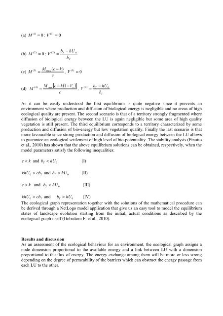
As it can be easily understood the first equilibrium is quite negative since it prevents an
environment where production and diffusion of biological energy is negligible and no areas of high
ecological quality are present. The second scenario is that of a territory strongly fragmented where
diffusion of biological energy between the LU is again negligible but some area of high quality
vegetation is still present. The third equilibrium corresponds to a territory characterized by some
production and diffusion of bio-energy but low vegetation quality. Finally the last scenario is that
more favourable since strong production and diffusion of biological energy between the LU allows
to guarantee an ecological settlement of high level of bio-potentiality. The stability analysis (Finotto
et al., 2010) has shown that the above equilibrium solutions can be obtained, respectively, when the
model parameters satisfy the following inequalities:
c < k and b T
< hU
0
(I)
khU
0
> cb T
and b T
> hU
0
(II)
c > k and b T
< hU
0
(III)
khU
0
> cb T
and b T
> hU
0
(IV)
The ecological graph representation together with the solutions of the mathematical procedure can
be derived through a NetLogo model application that give us an easy tool to model the equilibrium
states of landscape evolution starting from the initial, actual conditions as described by the
ecological graph itself (Gobattoni F. et al., 2010).
Results and discussion
As an assessment of the ecological behaviour for an environment, the ecological graph assigns a
node dimension proportional to the available energy and a link between LU with a dimension
proportional to the flux of energy. The energy exchange among them will be more or less strong
depending on the degree of permeability of the barriers which can obstruct the energy passage from
each LU to the other.