(TESTATE AMOEBAE) AND FORAMINIFERA FROM THREE ...
(TESTATE AMOEBAE) AND FORAMINIFERA FROM THREE ...
(TESTATE AMOEBAE) AND FORAMINIFERA FROM THREE ...

Create successful ePaper yourself
Turn your PDF publications into a flip-book with our unique Google optimized e-Paper software.
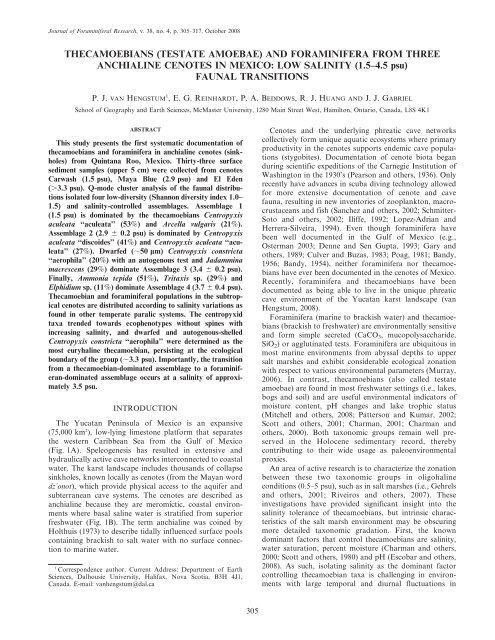
Journal of Foraminiferal Research, v. 38, no. 4, p. 305–317, October 2008<br />
THECAMOEBIANS (<strong>TESTATE</strong> <strong>AMOEBAE</strong>) <strong>AND</strong> <strong>FORAMINIFERA</strong> <strong>FROM</strong> <strong>THREE</strong><br />
ANCHIALINE CENOTES IN MEXICO: LOW SALINITY (1.5–4.5 psu)<br />
FAUNAL TRANSITIONS<br />
P. J. VAN HENGSTUM 1 ,E.G.REINHARDT, P.A.BEDDOWS, R.J.HUANG <strong>AND</strong> J. J. GABRIEL<br />
School of Geography and Earth Sciences, McMaster University, 1280 Main Street West, Hamilton, Ontario, Canada, L8S 4K1<br />
ABSTRACT<br />
This study presents the first systematic documentation of<br />
thecamoebians and foraminifera in anchialine cenotes (sinkholes)<br />
from Quintana Roo, Mexico. Thirty-three surface<br />
sediment samples (upper 5 cm) were collected from cenotes<br />
Carwash (1.5 psu), Maya Blue (2.9 psu) and El Eden<br />
(.3.3 psu). Q-mode cluster analysis of the faunal distributions<br />
isolated four low-diversity (Shannon diversity index 1.0–<br />
1.5) and salinity-controlled assemblages. Assemblage 1<br />
(1.5 psu) is dominated by the thecamoebians Centropyxis<br />
aculeata ‘‘aculeata’’ (53%) and Arcella vulgaris (21%).<br />
Assemblage 2 (2.9 6 0.2 psu) is dominated by Centropyxis<br />
aculeata ‘‘discoides’’ (41%) and Centropyxis aculeata ‘‘aculeata’’<br />
(27%). Dwarfed (,50 mm) Centropyxis constricta<br />
‘‘aerophila’’ (20%) with an autogenous test and Jadammina<br />
macrescens (29%) dominate Assemblage 3 (3.4 6 0.2 psu).<br />
Finally, Ammonia tepida (51%), Tritaxis sp. (29%) and<br />
Elphidium sp. (11%) dominate Assemblage 4 (3.7 6 0.4 psu).<br />
Thecamoebian and foraminiferal populations in the subtropical<br />
cenotes are distributed according to salinity variations as<br />
found in other temperate paralic systems. The centropyxid<br />
taxa trended towards ecophenotypes without spines with<br />
increasing salinity, and dwarfed and autogenous-shelled<br />
Centropyxis constricta ‘‘aerophila’’ were determined as the<br />
most euryhaline thecamoebian, persisting at the ecological<br />
boundary of the group (,3.3 psu). Importantly, the transition<br />
from a thecamoebian-dominated assemblage to a foraminiferan-dominated<br />
assemblage occurs at a salinity of approximately<br />
3.5 psu.<br />
INTRODUCTION<br />
The Yucatan Peninsula of Mexico is an expansive<br />
(75,000 km 2 ), low-lying limestone platform that separates<br />
the western Caribbean Sea from the Gulf of Mexico<br />
(Fig. 1A). Speleogenesis has resulted in extensive and<br />
hydraulically active cave networks interconnected to coastal<br />
water. The karst landscape includes thousands of collapse<br />
sinkholes, known locally as cenotes (from the Mayan word<br />
dz’onot), which provide physical access to the aquifer and<br />
subterranean cave systems. The cenotes are described as<br />
anchialine because they are meromictic, coastal environments<br />
where basal saline water is stratified from superior<br />
freshwater (Fig. 1B). The term anchialine was coined by<br />
Holthuis (1973) to describe tidally influenced surface pools<br />
containing brackish to salt water with no surface connection<br />
to marine water.<br />
1<br />
Correspondence author. Current Address: Department of Earth<br />
Sciences, Dalhousie University, Halifax, Nova Scotia, B3H 4J1,<br />
Canada. E-mail: vanhengstum@dal.ca<br />
Cenotes and the underlying phreatic cave networks<br />
collectively form unique aquatic ecosystems where primary<br />
productivity in the cenotes supports endemic cave populations<br />
(stygobites). Documentation of cenote biota began<br />
during scientific expeditions of the Carnegie Institution of<br />
Washington in the 1930’s (Pearson and others, 1936). Only<br />
recently have advances in scuba diving technology allowed<br />
for more extensive documentation of cenote and cave<br />
fauna, resulting in new inventories of zooplankton, macrocrustaceans<br />
and fish (Sanchez and others, 2002; Schmitter-<br />
Soto and others, 2002; Iliffe, 1992; Lopez-Adrian and<br />
Herrera-Silveira, 1994). Even though foraminifera have<br />
been well documented in the Gulf of Mexico (e.g.,<br />
Osterman 2003; Denne and Sen Gupta, 1993; Gary and<br />
others, 1989; Culver and Buzas, 1983; Poag, 1981; Bandy,<br />
1956; Bandy, 1954), neither foraminifera nor thecamoebians<br />
have ever been documented in the cenotes of Mexico.<br />
Recently, foraminifera and thecamoebians have been<br />
documented as being able to live in the unique phreatic<br />
cave environment of the Yucatan karst landscape (van<br />
Hengstum, 2008).<br />
Foraminifera (marine to brackish water) and thecamoebians<br />
(brackish to freshwater) are environmentally sensitive<br />
and form simple secreted (CaCO 3 , mucopolysaccharide,<br />
SiO 2 ) or agglutinated tests. Foraminifera are ubiquitous in<br />
most marine environments from abyssal depths to upper<br />
salt marshes and exhibit considerable ecological zonation<br />
with respect to various environmental parameters (Murray,<br />
2006). In contrast, thecamoebians (also called testate<br />
amoebae) are found in most freshwater settings (i.e., lakes,<br />
bogs and soil) and are useful environmental indicators of<br />
moisture content, pH changes and lake trophic status<br />
(Mitchell and others, 2008; Patterson and Kumar, 2002;<br />
Scott and others, 2001; Charman, 2001; Charman and<br />
others, 2000). Both taxonomic groups remain well preserved<br />
in the Holocene sedimentary record, thereby<br />
contributing to their wide usage as paleoenvironmental<br />
proxies.<br />
An area of active research is to characterize the zonation<br />
between these two taxonomic groups in oligohaline<br />
conditions (0.5–5 psu), such as in salt marshes (i.e., Gehrels<br />
and others, 2001; Riveiros and others, 2007). These<br />
investigations have provided significant insight into the<br />
salinity tolerance of thecamoebians, but intrinsic characteristics<br />
of the salt marsh environment may be obscuring<br />
more detailed taxonomic gradation. First, the known<br />
dominant factors that control thecamoebians are salinity,<br />
water saturation, percent moisture (Charman and others,<br />
2000; Scott and others, 1980) and pH (Escobar and others,<br />
2008). As such, isolating salinity as the dominant factor<br />
controlling thecamoebian taxa is challenging in environments<br />
with large temporal and diurnal fluctuations in<br />
305
306 VAN HENGSTUM <strong>AND</strong> OTHERS<br />
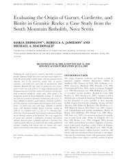
FIGURE 1. A Study sites. The coastline is marked by the thick black<br />
line, roads by medium lines and topographic elevations by thin black<br />
lines. Note that this is not a complete list of local cenotes. B Idealized<br />
model of an anchialine karst system on the Yucatan Peninsula.<br />
multiple parameters. Second, soil thecamoebian taxa<br />
become established in extreme high marsh zone where<br />
pedogenic processes begin, and these taxa have the<br />
potential to taphonomically bias lower salt marsh assemblages.<br />
This problem further confounds attempts to isolate<br />
gradations from the lacustrine thecamoebians to foraminifera<br />
with increasing salinity. Third, the sharp faunal<br />
gradations observed in salt marshes are not as intergradational<br />
as desired to observe thecamoebian taxonomic<br />
subtleties (Gehrels and others, 2001). As such, additional<br />
environments are needed to further study these faunal<br />
transitions. Although salt marshes cannot be directly<br />
compared to cenotes due to the many differences between<br />
these two environments, the oligohaline cenote may be<br />
another setting in conjunction with salt marshes to resolve<br />
low salinity effects on thecamoebians and foraminifera. The<br />
objectives of this study were to (1) characterize and develop<br />
baseline data on distributions of thecamoebians and<br />
foraminifera in Yucatan anchialine cenotes and (2)<br />
investigate the species succession between thecamoebians<br />
and foraminifera in oligohaline conditions.<br />
CENOTE PHYSIOGRAPHY <strong>AND</strong> STUDY SITES<br />
The Yucatan Peninsula is composed of diagenetically<br />
immature reefal limestone with Eocene rock in the interior<br />
grading seaward to a Quaternary coastline overlain by<br />
unconsolidated Holocene sediments (Weidie, 1985). The<br />
limestone retains ,25% porosity (Harris, 1984) allowing<br />
effective infiltration and drainage of precipitation and<br />
subsequently contributes to a lack of rivers in the Yucatan.<br />
Speleogenesis has been an ongoing process on the Yucatan<br />
Peninsula since the late Neogene in both phreatic and<br />
vadose settings. The geologic processes controlling cenote<br />
formation are (1) sub-aerial dissolution of limestone in the<br />
vadose zone through carbonic acid percolation during<br />
precipitation; (2) subterranean dissolution and collapse of<br />
cave ceilings from karst dissolution at the CO 3<br />
22<br />
undersaturated<br />
halocline (Smart and others, 1988); and (3)<br />
dominantly through the collapse of cave ceilings due to<br />
the removal of a hydraulic buoyant force during sea level<br />
regressions (Smart and others, 2006; Schmitter-Soto and<br />
others, 2002). Cenote morphology most commonly contains<br />
a circular or elliptical opening with limestone blocks<br />
forming a central breakdown pile on the cenote floor<br />
(Fig. 1B). Sediment accumulations at the bottom of the<br />
cenote have been recently investigated by Gabriel and<br />
others (in press) and determined to record environmental<br />
evolution in the cenote.<br />
The eastern Yucatan receives a mean annual rainfall of<br />
1.5 m/yr, with up to 85% lost through evapotranspiration<br />
based on calculations from mean annual air temperatures.<br />
The remaining 15% of annual rainfall is drained through<br />
the freshwater lens (Alcocer and others, 1998; Moore and<br />
others, 1992; Hanshaw and Back, 1980). The modern<br />
aquifer on the Yucatan is density-stratified; a freshwater<br />
lens is buoyant and floats above the marine water intruding<br />
from the coast (Moore and others, 1992). Both fresh and<br />
saline waters circulate through the caves at 1–10 km/day.<br />
While the fresh water in the lens actively migrates<br />
coastward, the marine water incursion exhibits diurnal<br />
landward migration within larger subsurface convection<br />
cells (Beddows and others, 2007; Moore and others, 1992).<br />
The halocline separating the fresh and marine water<br />
dissolves the limestone in a phreatic setting, resulting in<br />
anastomosing, phreatic caves (Smart and others, 1988;<br />
2006). Sea level oscillations throughout the Neogene have<br />
regularly shifted the relative position of the halocline,<br />
subsequently causing cave development at different elevations<br />
in the subsurface. Local variations in hydrogeology<br />
throughout the Yucatan cause significant variability in<br />
cenote water chemistry (e.g., pH: 6.3–10.4, dissolved<br />
oxygen: 0.6–7.4 mL L 21 , temperature: 22–33.5uC, chlorophyll-a:<br />
0.11–97.4 mg/m 3 ; Schmitter-Soto and others, 2002).<br />
CARWASH CENOTE<br />
The Carwash Cenote (CW) is the main access into the<br />
Aktun Ha (Carwash) Cave System, located ,8.5 km west<br />
of the Caribbean coast, within 40 m of the highway<br />
(Fig 1A). The sinkhole has an elliptical opening with an<br />
average length of 46 m, width of 15 m and depth of 5 m<br />
(Fig. 3). The submerged central breakdown pile on the<br />
bottom is generally flat, with only one large boulder located<br />
in the northern end of the sinkhole, although there are<br />
many submerged tree trunks and branches around the<br />
periphery. The sediment accumulation on the breakdown<br />
pile and the cenote response to rising Holocene sea-level<br />
was documented by Gabriel and others (in press) and the<br />
deeper cave thecamoebians and foraminifera in van<br />
Hengstum and others (in press). The benthic environment
OLIGOHALINE FAUNA IN MEXICAN CENOTES 307<br />
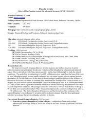
FIGURE 2. Depth profiles of hydrologic variables (salinity, pH,<br />
dissolved oxygen, temperature) through the aquifer at each cenote site.<br />
The shadowed region represents the halocline at the different locales.<br />
contains a dense cover of algal mats and abundant fish<br />
(especially Astyanax mexicanus). During the rainy season,<br />
algal blooms characterize the surface water, where active<br />
primary productivity creates vibrant green surface water.<br />
Dissolved oxygen (2.4 ml L 21 ) is above the ecological<br />
requirements of most aerobic foraminifera (.1 mlL 21 ),<br />
but the salinity of 1.5 psu inhibits most taxa (Murray,<br />
2006). The top of the local halocline is seasonally stationary<br />
at 21 m depth, which is significantly below the range of<br />
sampling depths (Fig. 2). Detailed water-quality data for<br />
the Carwash Cenote is given in Alcocer and others (1998).<br />
MAYA BLUE CENOTE<br />
The Maya Blue Cenote (MB) is one of several sinkholes<br />
in the Naranjal-Maya Blue Cave System, located ,5.6 km<br />
west of the Caribbean coast (Fig. 1A). The water-filled<br />
sinkhole is crescent-shaped, with an average length of 50 m,<br />
width of 10 m and depth of 3.5 m. Large blocks of<br />
limestone ,6–10 m in width are exposed at the bottom<br />
and are interspersed with sediment that is visibly abundant<br />
in diatoms and organic matter. A larger area of exposed<br />
sediment occurs at the center of the cenote, where several<br />
macrophytes have become established. The Maya Blue<br />
Cenote is more oligotrophic than the Carwash Cenote, with<br />
a notable absence of reoccurring pelagic algal blooms and<br />
year-round water clarity. Salinity is 2.9 psu, and dissolved<br />
oxygen is above the normal metabolic requirements for<br />
foraminifera in the range of sampling depths.<br />
FIGURE 3. Map of cenote morphology with locations of surface<br />
sediment samples.<br />
EL EDEN CENOTE<br />
El Eden Cenote (EE) is situated 1.8 km inland from the<br />
Caribbean coast and is a popular tourist snorkeling<br />
attraction in Quintana Roo (Fig. 1). The cenote averages<br />
37 m by 15 m in length and width and is one of several<br />
cenotes found in the larger Ponderosa Cave System. Large<br />
blocks of limestone strata, collapsed during cenote formation,<br />
characterize the benthic environment. Along the<br />
periphery, a few of these limestone blocks intersect the<br />
water interface and have developed into miniature islands<br />
colonized by ferns and grasses. This creates a high degree of<br />
variability in depths across the cenote bottom from 1 to<br />
8 m. The diversity of fish fauna is greater at El Eden Cenote<br />
compared to the other two cenotes. The halocline is the<br />
shallowest at this locale, being at 11.5 m depth, with a<br />
subtly increasing salinity from the surface (3.3 psu) to the<br />
halocline. Dissolved oxygen (.2.0 ml L 21 ) and hydrologic<br />
flow rates (3 cm/s) of the freshwater lens are greater at El<br />
Eden Cenote as compared to the other two sites. The<br />
configuration of the breakdown blocks, which range down
308 VAN HENGSTUM <strong>AND</strong> OTHERS<br />
into the saline water, combined with increased flow rates,<br />
visibly induce turbulence and enhanced mixing of the saline<br />
water into the freshwater lens at El Eden Cenote.<br />
METHODS <strong>AND</strong> ANALYSIS<br />
Thirty-three surface sediment samples (upper 5 cm) were<br />
collected from the Carwash Cenote (CW; n 5 7), the Maya<br />
Blue Cenote (MB; n 5 12) and El Eden Cenote (EE; n 5 14)<br />
by scuba diving in August 2006 (Fig. 3), capturing the<br />
range of cenote subenvironments. Depth profiles of salinity,<br />
pH, dissolved oxygen and temperature were collected<br />
through the aquifer at each cenote locale with a submersible<br />
multi-parameter probe (YSI 600XLM) to characterize<br />
current hydrologic conditions. Sediment samples were<br />
washed on a 45-mm screen to retain thecamoebians and<br />
foraminifera. Remaining sediment residues were wet-split<br />
as required and all samples were picked wet. Thecamoebian<br />
taxonomy generally follows Medioli and Scott (1983) and<br />
Reinhardt and others (1998). A total of eight thecamoebian<br />
and eleven foraminifera taxa were identified in the three<br />
cenotes (Plate 1, Table 1). Thecamoebians and foraminifera<br />
were considered collectively in this study, where relative<br />
fractional abundance (F i ) of each taxonomic unit was<br />
calculated by<br />
F i ~ C i<br />
N i<br />
,<br />
where C i is the number of specimens of a species counted<br />
and N i is the total number of specimens counted in the<br />
sample.<br />
As an exploratory tool, shell categories (thecamoebians,<br />
agglutinated foraminifera and calcite foraminifera) were<br />
plotted on a ternary diagram, a useful technique to describe<br />
different foraminiferal environments (i.e., Murray, 2006).<br />
With thecamoebians, agglutinated foraminifera and calcite<br />
foraminifera representing the lacustrine to marine salinity<br />
continuum, a ternary diagram can provide insight into the<br />
distributions in environments with the most marginal<br />
salinity. The recovered taxa were categorized as above<br />
using the fractional abundance and plotted on a standard<br />
ternary diagram.<br />
The standard error (S Fi ) of sampling (for a two-tailed<br />
alpha of 0.05) for each taxon was used to determine<br />
statistically significant taxa. If the calculated standard error<br />
for a taxon was greater than the fractional abundance in all<br />
the samples, then that that particular taxon was deemed<br />
statistically insignificant and excluded from further multivariate<br />
analysis (Patterson and Fishbein, 1989). Standard<br />
error was calculated through the following formula, where t<br />
is Student’s t:<br />
sffiffiffiffiffiffiffiffiffiffiffiffiffiffiffiffiffiffiffiffiffiffi<br />
F i ð1 { F i Þ<br />
~ t1<br />
,<br />
S Fi<br />
Additionally, the Shannon-Weaver diversity index (SDI;<br />
Shannon and Weaver, 1949) was calculated for each sample<br />
to quantify the environmental stability at each sample<br />
location (stable conditions are .2.5, transitional conditions<br />
are 1.5–2.5 and ‘harsh’ conditions are ,1.5; Patterson and<br />
N i<br />
Kumar, 2002). Although these ranges were used by<br />
Patterson and Kumar (2002) exclusively for thecamoebians,<br />
Riveiros and others (2007) used these SDI ranges to<br />
successfully describe collective thecamoebian and foraminiferal<br />
assemblages from a Canadian salt marsh. Since the<br />
SDI is strongly influenced by the species richness in a<br />
sample and in oligohaline settings the species richness of<br />
both thecamoebians and foraminifera decreases, the meaning<br />
of the numeric ranges presented by Patterson and<br />
Kumar (2002) is preserved in oligohaline conditions. The<br />
index is calculated through the following formula, where S<br />
is the species richness for each sample:<br />
SDI ~{ XS l<br />
<br />
F i<br />
N i<br />
<br />
1ln<br />
F i<br />
N i<br />
Q-mode cluster analysis is used to characterize statistically<br />
similar assemblages using the statistical freeware<br />
package PAST (Hammer and others, 2001). Of the total<br />
21 taxonomic units recovered, three thecamoebian taxa<br />
(Bullinularia indica, Difflugia oblonga, Lagenodifflugia vas)<br />
and two foraminiferan taxa (Bolivina variabilis and<br />
Textularia earlandi) were statistically insignificant due to<br />
large standard error and therefore omitted from further<br />
multivariate analysis (Patterson and Fishbein, 1989).<br />
Samples were compared using a simple Euclidean distance<br />
coefficient and amalgamated into clusters using Ward’s<br />
method of minimum variance; the results are displayed in<br />
an hierarchical dendrogram (Fig. 4). The biocoenosis was<br />
not quantified, but the combined bio- and thanatocoenosis<br />
is thought to better characterize average conditions at a<br />
sample site (Osterman, 2003; Scott and Medioli, 1980a).<br />
RESULTS<br />
The dendrogram produced by the Q-mode cluster<br />
analysis indicates four distinct salinity-controlled clusters<br />
that are interpreted as separate assemblages (Fig. 4). All<br />
seven samples recovered from CW form Assemblage 1 (A1)<br />
with a mean depth of 4.6 m and a salinity of 1.5 psu. A1 is<br />
characterized by abundant Centropyxis aculeata (74%) and<br />
Arcella vulgaris (21%). Notably, the thecamoebian strain C.<br />
aculeata ‘‘aculeata’’ (with spines, 53%) dominates over the<br />
strain without spines, C. aculeata ‘‘discoides’’ (21%). Only<br />
one sample in CW contains a small number of Jadammina<br />
macrescens (2%). Very low diversity (mean SDI 5 1.05,<br />
Table 2) indicates the environment deviates from optimal<br />
growth conditions for both lacustrine testate amoebae and<br />
foraminifera (where SDI .2). On the ternary diagram, all<br />
the samples plot at or near the apex due to the large relative<br />
abundance of thecamoebians (mean 99.6%; Fig. 5).<br />
The majority of samples from Assemblage 2 (A2) come<br />
from MB. The A2 samples were found at a mean depth of<br />
3.5 m and a salinity of 2.9 6 0.2 psu. Centropyxid taxa<br />
dominate (mean 82%), however, there are subtle taxonomic<br />
shifts at the species and strain (ecophenotype) level.<br />
Centropyxis aculeata ‘‘aculeata’’ decreases (mean 27%),<br />
whereas C. aculeata ‘‘discoides’’ increases (41%). There is a<br />
significant decrease in the contribution of Arcella vulgaris<br />
(mean 2 6 3%; high SD due to larger inter-sample variability)<br />
to the populations compared to that in A1. Centropyxis
OLIGOHALINE FAUNA IN MEXICAN CENOTES 309<br />
TABLE 1.<br />
Relative abundance and standard error (61 s) for taxonomic units.<br />
Sample E1 E2 E3 E5 E6 E7 E8 E9 E10 E11<br />
Depth (m) 3.4 6.4 1.8 5 3 4 2.1 5.5 2.4 1.8<br />
Salinity (psu) 3.5 4.2 3.4 3.7 3.5 3.6 3.4 4 3.5 3.4<br />
Sum (N i ) 331 179 327 496 259 394 1075 462 219 193<br />
Individuals/cc 26 24 131 50 104 79 430 185 88 25<br />
Shannon diversity index (H) 1.965 1.187 1.28 1.078 0.997 1.232 1.529 1.41 1.143 1.666<br />
Arcella vulgaris 1.81 - 0.61 - 1.93 - 0.28 1.52 - 3.63<br />
standard error (6) 1.44 - 0.85 - 1.68 - 0.32 1.11 - 2.64<br />
Bullinularia indica - - - - - - - - - -<br />
standard error (6) - - - - - - - - - -<br />
Centropyxis aculeata ‘‘aculeata’’ 3.63 0.56 9.17 - 4.63 1.02 3.91 2.81 12.79 4.15<br />
standard error (6) 2.01 1.09 3.13 - 2.56 0.99 1.16 1.51 4.42 2.81<br />
Centropyxis aculeata ‘‘discoides’’ 1.21 1.12 6.12 0.81 76.45 1.52 3.26 1.73 6.39 26.42<br />
standard error (6) 1.18 1.54 2.60 0.79 5.17 1.21 1.06 1.19 3.24 6.22<br />
Centropyxis constricta ‘‘aerophila’’ 29.91 0.56 - - 5.02 - 19.72 - 3.65 1.04<br />
standard error (6) 4.93 1.09 - - 2.66 - 2.38 - 2.48 1.43<br />
Centropyxis constricta ‘‘constricta’’ 14.80 - 0.31 0.20 2.32 - 0.09 - 0.91 -<br />
standard error (6) 3.83 - 0.60 0.39 1.83 - 0.18 - 1.26 -<br />
Difflugia globulus - - - - - - - - - -<br />
standard error (6) - - - - - - - - - -<br />
Difflugia oblonga - - - - - - - - - -<br />
standard error (6) - - - - - - - - - -<br />
Lagenodifflugia vas - - - - - - - - - -<br />
standard error (6) - - - - - - - - - -<br />
Ammonia tepida var. juvenile 0.30 - 0.61 - - - 0.84 - - -<br />
standard error (6) 0.59 - 0.85 - - - 0.54 - - -<br />
Ammonia tepida 25.68 58.66 66.06 48.59 5.41 44.42 13.77 51.95 0.46 38.86<br />
standard error (6) 4.71 7.21 5.13 4.40 2.75 4.91 2.06 4.56 0.89 6.88<br />
Bolivina striatula 3.63 - - - - - - 1.30 - -<br />
standard error (6) 2.01 - - - - - - 1.03 - -<br />
Bolivina variabilis 0.30 - - - - - - - - -<br />
standard error (6) 0.59 - - - - - - - - -<br />
Elphidium sp. 3.02 2.23 4.28 36.69 2.70 10.66 1.30 14.94 - 6.22<br />
standard error (6) 1.84 2.17 2.19 4.24 1.97 3.05 0.68 3.25 - 3.41<br />
Miliammina fusca 1.21 3.91 7.65 - 0.39 2.79 5.30 2.60 9.13 1.04<br />
standard error (6) 1.18 2.84 2.88 - 0.76 1.63 1.34 1.45 3.82 1.43<br />
Polysaccammina iophalina 0.30 - - - - - 0.09 - 0.46 -<br />
standard error (6) 0.59 - - - - - 0.18 - 0.89 -<br />
Rosalina subaracuana - 2.79 0.61 - - - - - - -<br />
standard error (6) - 2.41 0.85 - - - - - - -<br />
Spirillina vivipara - - - - - - - - - -<br />
standard error (6) - - - - - - - - - -<br />
Textularia earlandi 0.60 - - - - - - - - -<br />
standard error (6) 0.83 - - - - - - - - -<br />
Triloculina oblonga 0.60 - - - - - - - - 0.52<br />
standard error (6) 0.83 - - - - - - - - 1.01<br />
Tritaxis fusca 2.72 27.37 2.14 12.70 0.77 38.32 1.67 21.43 - 14.51<br />
standard error (6) 1.75 6.53 1.57 2.93 1.07 4.80 0.77 3.74 - 4.97<br />
Jadammina macrescens 10.27 2.79 2.45 1.01 0.39 1.27 49.77 1.73 66.21 3.63<br />
standard error (6) 3.27 2.41 1.67 0.88 0.76 1.11 2.99 1.19 6.26 2.64<br />
constricta ‘‘aerophila’’ (mean 9%) andCentropyxis constricta<br />
‘‘spinosa’’ (mean 3%) increase as compared to A1, but the<br />
tests of this species are exceptionally dwarfed, and only<br />
autogenous tests were found. The absence of xenogenous<br />
tests is interesting, as this type of test is very abundant in<br />
other lacustrine settings (i.e., see Patterson and Kumar,<br />
2002). The euryhaline agglutinated foraminifera Jadammina<br />
macrescens (mean 9%) andMiliammina fusca (mean 4%) are<br />
present in A2, placing these samples along the left axis on the<br />
ternary plot (Fig. 5). As in A1, optimal growth conditions are<br />
not present as indicated by the low diversity (mean SDI 5<br />
1.367).<br />
Assemblage 3 (A3) contains six samples from EE and one<br />
sample from MB. The average depth for the samples from<br />
EE is 2.5 m and the sample from MB comes from a depth<br />
of 1.8 m (M7). The mean salinity for all samples is 3.4 6<br />
0.2 psu, and faunal diversity remains low (mean SDI 5<br />
1.509), albeit slightly more elevated than the other<br />
assemblages, indicating faunal populations are experiencing<br />
some ecological stress. The centropyxid taxa continue to<br />
decrease in dominance (mean 48%), agglutinated foraminifera<br />
increase (mean 36%) and calcite foraminifera (mean<br />
14%) are present relative to A1 and A2. The relative<br />
contribution of these taxa to the assemblage skews the<br />
position of the samples to the bottom left and center of the<br />
ternary diagram (Fig. 5). Centropyxis aculeata is no longer<br />
a dominant species in A3, and the abundance of the<br />
dwarfed Centropyxis constricta doubles (mean 28%). The<br />
abundance of Jadammina macrescens (30%) and Miliammina<br />
fusca (3%) also increase. Tritaxis sp. (mean 4 6 4%)
310 VAN HENGSTUM <strong>AND</strong> OTHERS<br />
TABLE 1.<br />
Continued.<br />
Sample E13 E14 E15 M1 M2 M3 M4 M5 M6 M7<br />
Depth (m) 2.7 2.1 6.7 1.8 4.9 1.8 5.49 2.7 4 1.8<br />
Salinity (psu) 3.5 3.4 4.4 2.9 2.9 2.9 2.9 2.9 2.9 2.9<br />
Sum (N i ) 215 93 242 382 234 233 328 162 246 253<br />
Individuals/cc 29 37 24 306 187 186 328 162 246 204<br />
Shannon diversity index (H) 1.977 1.124 1.139 1.625 1.242 1.146 1.298 1.277 1.731 1.049<br />
Arcella vulgaris 2.33 - - 0.52 - 9.01 - - 0.41 0.40<br />
standard error (6) 2.01 - - 0.72 - 3.68 - - 0.80 0.77<br />
Bullinularia indica - - - 0.52 - - - - - -<br />
standard error (6) - - - 0.72 - - - - - -<br />
Centropyxis aculeata ‘‘aculeata’’ 8.84 12.90 0.41 25.39 12.82 4.72 40.85 20.37 13.82 13.83<br />
standard error (6) 3.79 6.89 0.81 4.36 4.28 2.72 5.32 6.20 4.31 4.25<br />
Centropyxis aculeata ‘‘discoides’’ 5.58 3.23 - 35.60 59.83 64.38 38.11 55.56 34.15 0.40<br />
standard error (6) 3.07 3.63 - 4.80 6.28 6.15 5.26 7.65 5.93 0.77<br />
Centropyxis constricta ‘‘aerophila’’ 20.93 - - 19.37 3.42 16.31 13.41 14.20 17.48 50.99<br />
standard error (6) 5.44 - - 3.96 2.33 4.74 3.69 5.37 4.75 6.16<br />
Centropyxis constricta ‘‘constricta’’ 31.16 - 0.41 8.64 1.71 4.29 3.35 1.85 3.25 33.99<br />
standard error (6) 6.19 - 0.81 2.82 1.66 2.60 1.95 2.08 2.22 5.84<br />
Difflugia globulus - - - - - 0.43 0.30 - 0.41 -<br />
standard error (6) - - - - - 0.84 0.60 - 0.80 -<br />
Difflugia oblonga - - - - - - - - - -<br />
standard error (6) - - - - - - - - - -<br />
Lagenodifflugia vas - - - - - - 0.30 - - -<br />
standard error (6) - - - - - - 0.60 - - -<br />
Ammonia tepida var. juvenile 0.47 - 0.41 0.52 - - - - 0.41 -<br />
standard error (6) 0.91 - 0.81 0.72 - - - - 0.80 -<br />
Ammonia tepida 11.16 19.35 49.59 - - - - 0.62 - -<br />
standard error (6) 4.21 8.12 6.30 - - - - 1.21 - -<br />
Bolivina striatula - - - - - - - - - -<br />
standard error (6) - - - - - - - - - -<br />
Bolivina variabilis - - - - - - - - - -<br />
standard error (6) - - - - - - - - - -<br />
Elphidium sp. - - 2.48 - 1.71 - - - 1.22 -<br />
standard error (6) - - 1.96 - 1.66 - - - 1.37 -<br />
Miliammina fusca 1.86 - - 4.97 17.09 0.43 2.13 3.70 17.07 -<br />
standard error (6) 1.81 - - 2.18 4.82 0.84 1.56 2.91 4.70 -<br />
Polysaccammina iophalina 2.33 2.15 - - - - - - - -<br />
standard error (6) 2.01 2.98 - - - - - - - -<br />
Rosalina subaracuana - - - - - - - - - -<br />
standard error (6) - - - - - - - - - -<br />
Spirillina vivipara - - 0.83 - - - - - - -<br />
standard error (6) - - 1.14 - - - - - - -<br />
Textularia earlandi - - - - - - - - - -<br />
standard error (6) - - - - - - - - - -<br />
Triloculina oblonga 0.47 - - - - - - - - -<br />
standard error (6) 0.91 - - - - - - - - -<br />
Tritaxis fusca 3.72 1.08 36.36 0.26 - - - - - -<br />
standard error (6) 2.53 2.12 6.06 0.51 - - - - - -<br />
Jadammina macrescens 11.16 61.29 9.50 4.19 3.42 0.43 1.52 3.70 11.79 0.40<br />
standard error (6) 4.21 10.01 3.70 2.01 2.33 0.84 1.33 2.91 4.03 0.77<br />
and Ammonia tepida (mean 13 6 10%) contribute to<br />
populations, but there is large intra-sample variability.<br />
Aberrant tests were recorded in four samples (E1, E8, E10,<br />
E12), where 2% of Ammonia tepida, 35% of Elphidium sp.<br />
and 5% of J. macrescens had irregular test morphologies.<br />
All samples from Assemblage 4 (A4) come from EE at a<br />
mean depth of 4.5 m and salinity of 3.7 6 0.4 psu.<br />
Thecamoebian taxa decrease significantly (mean 9%) with<br />
large intra-sample variability (6 13%). Ammonia tepida<br />
(mean 51%) is the dominant taxon, with Tritaxis sp. (21%)<br />
and Elphidium sp. (mean 11 6 12%) contributing to the<br />
assemblage and increasing the diversity. The dominance of<br />
hyaline foraminifera in A4 causes the samples to plot in the<br />
lower right apex of the ternary diagram. Diversity is low (SDI<br />
5 1.284) from continual environmental stress in the low<br />
salinity conditions. In samples where test aberrancy was<br />
recorded (E5, E7, E9), 17% of Elphidium sp. contained<br />
irregular chambers and 25% of Jadammina macrescens in E9.<br />
DISCUSSION<br />
COMPARISON BETWEEN CENOTES<br />
The greatest dominance of thecamoebians occurs in CW<br />
(mean 99.6%), which is to be expected, as this cenote has<br />
salinity (1.5 psu) values closest to the ideal thecamoebian<br />
habitat of fresh water. In the ternary diagram, all the<br />
samples from CW plot at the apex, reflecting the dominance
OLIGOHALINE FAUNA IN MEXICAN CENOTES 311<br />
TABLE 1.<br />
Continued.<br />
Sample M9 M10 M11 M12 C1 C2 C3 C4 C5 C6<br />
Depth (m) 3.6 2.4 4.6 2.4 5.5 4.9 4.6 4.3 3 5.9<br />
Salinity (psu) 2.9 2.9 2.9 2.9 1.5 1.5 1.5 1.5 1.5 1.5<br />
Sum (N i ) 429 169 260 120 294 157 223 90 286 106<br />
Individuals/cc 343 135 208 96 78 31 45 29 57 84<br />
Shannon diversity index (H) 1.22 1.636 1.672 1.18 1.005 0.901 1.0379 0.924 1.174 1.037<br />
Arcella vulgaris - 4.14 2.31 5.83 38.78 5.73 21.08 31.11 20.98 14.15<br />
standard error (6) - 3.00 1.83 4.19 5.57 3.64 5.35 9.67 4.72 6.71<br />
Bullinularia indica - - 0.38 - - - - - - -<br />
standard error (6) - - 0.75 - - - - - - -<br />
Centropyxis aculeata ‘‘aculeata’’ 34.27 35.50 40.00 56.67 48.98 63.69 52.91 57.78 52.45 62.26<br />
standard error (6) 4.49 7.21 5.95 8.87 5.71 7.52 6.55 10.32 5.79 9.33<br />
Centropyxis aculeata ‘‘discoides’’ 46.15 14.20 22.69 21.67 11.56 28.03 25.56 11.11 22.38 19.81<br />
standard error (6) 4.72 5.26 5.09 7.37 3.65 7.03 7.73 6.57 4.83 7.67<br />
Centropyxis constricta ‘‘aerophila’’ 12.82 5.33 5.00 - - 2.55 - - - 2.83<br />
standard error (6) 3.16 3.39 2.65 - - 2.46 - - - 3.19<br />
Centropyxis constricta ‘‘constricta’’ 4.43 2.96 5.38 2.50 0.34 - 0.45 - - -<br />
standard error (6) 1.95 2.55 2.74 2.79 0.67 - 0.88 - - -<br />
Difflugia globulus - 4.73 1.54 - - - - - - -<br />
standard error (6) - 3.20 1.50 - - - - - - -<br />
Difflugia oblonga - - - - - - - - - -<br />
standard error (6) - - - - - - - - - -<br />
Lagenodifflugia vas - - - - - - - - 0.70 0.94<br />
standard error (6) - - - - - - - - 0.97 1.86<br />
Ammonia tepida var. juvenile 0.23 0.59 1.92 - - - - - 1.05 -<br />
standard error (6) 0.46 1.16 1.67 - - - - - 1.18 -<br />
Ammonia tepida - - - - - - - - - -<br />
standard error (6) - - - - - - - - - -<br />
Bolivina striatula - - - - - - - - - -<br />
standard error (6) - - - - - - - - - -<br />
Bolivina variabilis - - - - - - - - - -<br />
standard error (6) - - - - - - - - - -<br />
Elphidium sp. - - - - - - - - - -<br />
standard error (6) - - - - - - - - - -<br />
Miliammina fusca - 0.59 1.54 - - - - - - -<br />
standard error (6) - 1.16 1.50 - - - - - - -<br />
Polysaccammina iophalina - 0.59 0.77 - - - - - - -<br />
standard error (6) - 1.16 1.06 - - - - - - -<br />
Rosalina subaracuana - - - - - - - - - -<br />
standard error (6) - - - - - - - - - -<br />
Spirillina vivipara - - - - - - - - - -<br />
standard error (6) - - - - - - - - - -<br />
Textularia earlandi - - - - - - - - - -<br />
standard error (6) - - - - - - - - - -<br />
Triloculina oblonga - - - - - - - - - -<br />
standard error (6) - - - - - - - - - -<br />
Tritaxis fusca - - - - - - - - - -<br />
standard error (6) - - - - - - - - - -<br />
Jadammina macrescens 2.10 31.36 18.46 13.33 0.34 - - - 2.45 -<br />
standard error (6) 1.36 7.00 4.72 6.08 0.67 - - - 1.79 -<br />
of thecamoebians over foraminifera in that cenote (Fig. 5).<br />
One sample plots slightly down the left axis, reflecting the<br />
minor contribution of Jadammina macrescens at that<br />
sampling site. At MB, there is a larger contribution of<br />
agglutinated foraminifera (13%) causing the samples from<br />
that location to plot along the left axis of the ternary<br />
diagram. Thecamoebians are still the dominant fauna<br />
(85%) in MB, although the slightly higher salinity<br />
(2.9 psu) is more conducive to textularid populations than<br />
in CW. Since both of these cenotes have similar benthic<br />
conditions, hydrologic flow (1.5 cm/s), pH, oxygen and<br />
temperature (Fig. 2), the difference in salinity is likely the<br />
dominant abiotic factor contributing to the observed faunal<br />
variations.<br />
In contrast to MB and CW, the samples from EE are<br />
more evenly distributed over the ternary diagram than the<br />
other two cenotes. In addition to thecamoebians (mean<br />
28%) and agglutinated foraminifera (mean 29%), EE is also<br />
a habitat for calcite-shelled foraminifera (mean 43%). The<br />
halocline is shallowest at EE, and hydrologic flow is greater<br />
(3 cm/s) when compared to the other sites. The higher<br />
salinity at EE (.3.3 psu), associated with the proximity to<br />
the coast, allows euryhaline calcite taxa to become<br />
established (i.e., Ammonia tepida) and suppresses larger<br />
thecamoebian populations. Intra-sample variability can be<br />
explained in several ways: (1) subtle increases in salinity<br />
with depth in the freshwater lens; (2) complex bathymetry<br />
creating many microenvironments that might be influenced
312 VAN HENGSTUM <strong>AND</strong> OTHERS<br />
FIGURE 4. A Q-mode dendrogram indicating four distinct assemblages. The mean salinity with 1 standard deviation for each assemblage is<br />
provided. Sample labels follow those of Figure 3.<br />
TABLE 2.<br />
Average Shannon diversity index, salinity, dominant cenote of origin, depth and relative abundance for each taxon in the four assemblages.<br />
Assemblage 1 2 3 4<br />
Shannon diversity index (H) 1.034 1.367 1.509 1.284<br />
Salinity (psu) 1.5 2.9 6 0.2 3.4 6 0.2 3.7 6 0.4<br />
Dominant location of assemblage CW MB EE EE<br />
Mean sample depth (m) 4.6 3.5 2.5 4.5<br />
THECAMOEBIANS<br />
Arcella vulgaris 21 6 12 2 6 3 ,1 ,1<br />
Centropyxis aculeata ‘‘aculeata’’ 53 6 8 27 6 18 8 6 5 3 6 3<br />
Centropyxis aculeata ‘‘discoides’’ 21 6 6 41 6 19 3 6 2 5 6 9<br />
Centropyxis constricta ‘‘aerophila’’ ,1 3 6 1 20 6 17 ,1<br />
Centropyxis constricta ‘‘spinosa’’ ,1 9 6 6 15 6 15 ,1<br />
<strong>FORAMINIFERA</strong><br />
Jadammina macrescens 2 6 4 3 6 4 29 6 28 3 6 2<br />
Tritaxis sp. 0 ,1 3 6 4 21 6 13<br />
Ammonia tepida 0 ,1 13 6 10 51 6 9<br />
Elphidium sp. 0 ,1 ,1 11 6 12
OLIGOHALINE FAUNA IN MEXICAN CENOTES 313<br />
ASSEMBLAGE 2 (2.9 6 0.2 PSU)<br />
FIGURE 5. A ternary diagram showing the relative abundance of<br />
thecamoebians and foraminifera in the oligohaline cenote environment<br />
(,5 psu). The black arrow indicates the expected trajectory for<br />
assemblages under increasing salinity.<br />
through seasonal temperature changes; and (3) sediment resuspension<br />
and transport through tourist disturbance and<br />
higher hydrologic flow rates. These environmental variables<br />
are biologically relevant for amoebae, which can temporarily<br />
encyst during ecologically unfavorable conditions.<br />
Since these characteristics are not as prevalent at MB or<br />
CW as at EE, more consideration is given to these intrinsic<br />
characteristics when interpreting samples from EE.<br />
ASSEMBLAGE 1 (1.5 PSU)<br />
Assemblage 1 is located only at the CW, an environment<br />
suitable for only the most euryhaline of the thecamoebians.<br />
Therefore, Centropyxis aculeata dominates A1 and other<br />
more stenohaline thecamoebians are excluded (i.e., Difflugia<br />
oblonga ‘‘triangularis’’). The increased primary<br />
productivity in CW seems to promote the secondary<br />
dominance of Arcella vulgaris. This qualitative assessment<br />
is based on other studies where A. vulgaris becomes the<br />
dominant taxon when there is increased nutrient loading or<br />
primary productivity (Reinhardt and others, 2005). Rare<br />
Jadammina macrescens are also present with minimal test<br />
aberrancy, indicating some environmental stress on the<br />
species. These results are similar to those from other coastal<br />
and lacustrine studies in which (1) Centropyxis spp. are<br />
shown to be opportunists and the most euryhaline of the<br />
testate amoebae (i.e., Riveiros and others, 2007; Scott and<br />
others, 2001); (2) A. vulgaris is an indicator of environmental<br />
stress from nutrient loading (i.e., Roe and Patterson,<br />
2006; Reinhardt and others, 2005; Patterson and others,<br />
2002); and (3) rare J. macrescens persists at its ecological<br />
freshwater boundary of 1.5 psu (Murray, 2006).<br />
Between A1 and A2, there are taxonomic and environmental<br />
transitions. All the samples plot in the top-most<br />
region of the ternary diagram, indicating thecamoebians are<br />
still dominant contributors to the overall assemblage.<br />
Jadammina macrescens is still the only foraminiferan, with<br />
only a minor increase in abundance from A1. In the<br />
thecamoebians, there is a change in the dominant strain of<br />
the species Centropyxis aculeata. In the A2, there is a<br />
change to a dominance of C. aculeata ‘‘discoides’’ (41%)<br />
over C. aculeata ‘‘aculeata’’ (27%).<br />
The change to a dominance of Centropyxis aculeata<br />
‘‘discoides’’ over C. aculeata ‘‘aculeata’’ from A1 to A2 is a<br />
noteworthy observation. Reinhardt and others (1998)<br />
divided C. aculeata and Centropyxis constricta into<br />
ecophenotypes or ‘strains’ based on the presence or absence<br />
of spines: (1) C. aculeata ‘‘aculeata’’ is ornamented with<br />
spines on the aboral (fundus) region—we have observed up<br />
to 18; (2) C. aculeata ‘‘discoides’’ is circular, without spines;<br />
(3) C. constricta ‘‘aerophila’’ is lacking in spines on the<br />
aboral region; (4) C. constricta ‘‘constricta’’ is ornamented<br />
with 1–3 aboral spines; and (5) C. constricta ‘‘spinosa’’ is<br />
ornamented with .3 aboral spines. In previous lake studies,<br />
attributing these centropyxid strains to a definitive abiotic<br />
variable has proven problematic, although evidence does<br />
suggest that multiple environmental factors play a role in<br />
the phenotype expressed by a species (e.g., Reinhardt and<br />
others, 1998; Medioli and Scott, 1983).<br />
To retain consistency among the entire Centropyxis genus<br />
in this study, our taxonomic strain concept of C. aculeata is<br />
consistent with that of Reinhardt and others (1998), but C.<br />
constricta is modified as follows: (1) C. constricta ‘‘spinosa’’<br />
is characterized by the presence of aboral spines (we have<br />
observed up to 8); and (2) C. constricta ‘‘aerophila’’ is<br />
characterized by the absence of aboral spines. In A2, which<br />
has a slightly elevated salinity over A1, the C. aculeata test<br />
morphology without spines predominates (C. aculeata<br />
‘‘discoides’’). This relationship has also been observed in<br />
other global non-tropical settings. In the British Columbian<br />
salt marshes studied by Riveiros and others (2007), the<br />
ecophenotypes ‘‘discoides’’ (mean 12.5%) and ‘‘aerophila’’<br />
(14%) dominate over ‘‘aculeata’’ (7%) and ‘‘spinosa’’ (8%)<br />
in the saline-stressed High Marsh Assemblage. In UK salt<br />
marshes (Gehrels and others, 2001), C. constricta ‘‘aerophila’’<br />
(designated as C. platystoma, but reported by the<br />
authors as equivalent to the ‘‘aerophila’’ morphotype) is the<br />
most euryhaline of the thecamoebians (see Fig. 5 in Gehrels<br />
and others, 2001). These results indicate that in oligohaline<br />
environments, a thecamoebian ecophenotype without<br />
spines on the aboral region has an ecological advantage<br />
over their counterparts with spines. However, since spines<br />
are also expressed on thecamoebians in limnetic environments,<br />
other ecological or environmental factors may be<br />
controlling the expression of spines in the absence of stress<br />
related to salinity (such as pH, percent moisture or factors<br />
related to reproduction).<br />
ASSEMBLAGE 3 (3.4 6 0.2 PSU)<br />
Centropyxis constricta form the largest thecamoebian<br />
component (35%) in A3, with foraminifera emerging as the
314 VAN HENGSTUM <strong>AND</strong> OTHERS<br />
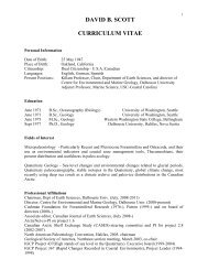
PLATE 1<br />
1–10 Thecamoebians: 1 Arcella vulgaris, autogenous test (x341); 2 A. vulgaris, (x341); 3 Centropyxis aculeata – xenogenous test (x406), note that the<br />
taxonomic criterion for angle between aperture face and body wall is to be ,45u (Medioli and Scott, 1983; x600); 4 C. constricta specimen with spines<br />
on xenogenous test (x300), note that the taxonomic criterion for angle between aperture face and body wall is to be .60u (Medioli and Scott, 1983;<br />
x600); 5 C. aculeata ‘‘aculeata’’ (x462); 6 C. aculeata ‘‘aculeata’’ (x388); 7 C. aculeata ‘‘discoides’’ (x462); 8 Impoverished and dwarfed C. constricta<br />
‘‘aerophila’’ with autogenous test (x425); 9 C. constricta ‘‘spinosa,’’ autogenous test (x300); 10 C. constricta ‘‘aerophila,’’ xenogenous test (x425). 11–<br />
26 Foraminifera: 11 Ammonia tepida, spiral side (x388); 12 A. tepida, umbilical side (x462); 13 A. tepida var. juvenile, proloculus and first two<br />
chambers, a consistent morphology (x775); 14 Ammonia tepida, aberrant test shape, arrow points to abnormal additional chamber (x150); 15<br />
Ammonia tepida, aberrant test shape, complex form (x150); 16 Elphidium sp. (x150); 17 Elphidium sp., aberrant test shape, arrow points to abnormal<br />
additional chamber (x150); 18. Elphidium sp. - aberrant test shape, complex form (x150); 19, 20 Miliammina fusca (x150); 21 Jadammina macrescens<br />
(x150); 22 J. macrescens, apertural view (x203); 23 J. macrescens, aberrant test displaying a twinned tests (x186); 24 Tritaxis sp., spiral view (x170); 25<br />
Tritaxis sp., umbilical view (x231); 26 Tritaxis sp., side view (x156). See Figure 4 of Geslin and others (2000) for categorization of morphological<br />
abnormalities. Scale bars represent 50 mm.
OLIGOHALINE FAUNA IN MEXICAN CENOTES 315<br />
dominant taxonomic grouping in the assemblage. Plate 1<br />
illustrates the separation of the species C. aculeata and C.<br />
constricta based on the geometric angle between the<br />
apertural face and the test wall (after Fig. 10 in Medioli<br />
and Scott, 1983; see Plate 1). In A3, the test of C. constricta<br />
is consistently autogenous; the strain without spines<br />
dominates the assemblage (C. constricta ‘‘aerophila’’,<br />
20%); and they have an overall dwarfed size (45–63 mm).<br />
As such, this morphotype of C. constricta ‘‘aerophila’’ is<br />
interpreted as the most euryhaline of the thecamoebians,<br />
persisting at the ecological boundary of the group. Again,<br />
we interpret the lack of spines in C. constricta ‘‘aerophila’’<br />
as physiologically advantageous over the ecophenotype<br />
with spines.<br />
The locations where A3 is recovered are more suitable<br />
habitats for foraminifera than A2 or A1, as indicated by an<br />
increase in the abundance of Jadammina macrescens (29%)<br />
and Tritaxis sp. (3%). Ammonia tepida and Elphidium sp.<br />
are also present, and the occurrence of aberrant tests<br />
indicates some ecological stress on these populations. The<br />
salinity increase from A2 to A3 is sufficient to make the<br />
environment more favorable for euryhaline foraminifera<br />
over thecamoebians. Longer-term salinity data in the<br />
cenote indicate very minor shifts over time (Beddows, in<br />
preparation), however, the shallow average depth for A3<br />
(,2.5 m) introduces the possibility of micro-environmental<br />
control on the distributions from the formation of<br />
seasonally-controlled cap layers of lower-salinity water.<br />
The fresher surface water during the rainy season would<br />
negatively affect the health of hyaline foraminifera, but<br />
positively affect thecamoebians (especially opportunists<br />
such as the centropyxids). In contrast, evaporation during<br />
the dry season would slightly increase salinity, creating<br />
conditions that are more favorable for foraminifera. This<br />
likely explains the small amount of C. aculeata in the<br />
assemblage and large intra-sample variability in the relative<br />
abundance of Elphidium sp. and Tritaxis sp. in A3. This<br />
assemblage represents the ecological boundary of thecamoebians<br />
in the cenotes.<br />
ASSEMBLAGE 4 (3.7 6 0.4 PSU)<br />
The most saline assemblage is A4 (mean 3.7 psu), in which<br />
foraminifera dominate and thecamoebians are only a minor<br />
contribution through Centropyxis aculeata (mean ,10%).<br />
Since this cenote is a popular tourist area (i.e., snorkeling,<br />
scuba diving) with appreciable hydrologic flow rates (3 cm/s),<br />
the possibility of thecamoebian tests being disturbed through<br />
recreational activity (post-mortem re-suspension) and transported<br />
to another deeper locale cannot be ignored. The<br />
reworking and transport of tests from shallower depths is a<br />
likely explanation of the variable abundance of thecamoebian<br />
tests in A4 and further explains the high intra-sample<br />
variability (standard deviations) in the mean abundance of<br />
taxa. The foraminifer Ammonia tepida (51%) dominates A4,<br />
an unsurprising result considering the adaptability of this<br />
genus and its reputation for being present in other oligohaline<br />
environments (i.e., Wennrich and others, 2007, and references<br />
therein). The second most abundant foraminifer in A4 is<br />
Tritaxis sp. (21%), an enigmatic observation as it is more<br />
commonly known from coastal shelves and bathyal sediments<br />
(e.g., Martin, 2008). It will be interesting to learn if more<br />
shelf-to-bathyal foraminifera are common in other mesohaline<br />
cenotes. The general trend in the cenotes of decreasing<br />
Jadammina macrescens and increasing abundance of other<br />
halophiles with increasing salinity is consistent with other<br />
reports of foraminiferal ecology (Scott and Medioli, 1978,<br />
1980b).<br />
The subtle salinity variation between A3 (mean 3.4 psu)<br />
and A4 (mean 3.7 psu) is due to the average sampling<br />
depths, where A3 is shallower (mean 2.5 m, mean of 51%<br />
total foraminifera in each sample) than A4 (mean 4.5 m,<br />
mean of 91% foraminifera in each sample). When<br />
comparing the three cenotes, the halocline is the shallowest<br />
at EE, and there is a subtle concomitant increase in salinity<br />
with depth (Fig. 2). The deeper saline water in EE is<br />
interpreted as a favorable environment for foraminifera and<br />
not thecamoebians, as apparent through larger abundances<br />
of foraminifera in A4. Future characterization of only the<br />
biocoenosis in the cenotes would likely decrease some of the<br />
variability in the different assemblages by eliminating<br />
taphonomic effects (i.e., excluding reworked specimens).<br />
Aberrant foraminiferal tests have been widely observed<br />
in response to anthropogenic influences such as pollution<br />
and natural variability in temperature, salinity, dissolved<br />
oxygen, pH, nutrition and other factors at the ecological<br />
boundary of a species (Geslin and others, 2000; Yanko and<br />
others, 1994; Boltovskoy and others, 1991). In the cenotes,<br />
dissolved oxygen, pH and temperature are all within the<br />
ecological requirements for healthy foraminiferal growth.<br />
The frequency of aberrant tests is fewer in the cenotes than<br />
in other studies (e.g., Wennrich and others, 2007), thereby<br />
suggesting only minor ecologic stress on the foraminiferal<br />
populations. However, the marginal salinities are interpreted<br />
as being the dominant ecological stress causing the<br />
observed test aberrancy.<br />
CONCLUSIONS<br />
Foraminifera and thecamoebians were recovered from<br />
the cenotes (sinkholes) on the Yucatan Peninsula, Mexico.<br />
The recovered foraminifera and thecamoebians (testate<br />
amoebae) from this subtropical setting are responding to<br />
local environmental controls in the same way as they do in<br />
previously investigated temperate systems. The anchialine<br />
nature of cenotes is an additional environment in which to<br />
study thecamoebian and foraminiferal ecology in oligohaline<br />
settings. In contrast to other coastal systems where<br />
thecamoebians and foraminifera co-occur, cenotes remain a<br />
permanently aquatic habitat with hydrology more stable<br />
than that in intertidal settings. Furthermore, cenotes remain<br />
energetically sheltered from large-scale, coastal perturbations<br />
(e.g., hurricanes), and microfossils in this environment<br />
are less exposed to taphonomic processes typical of neritic<br />
environments (e.g., wave action). Hence, thecamoebian<br />
populations in cenotes are dominantly influenced by<br />
aquatic conditions, as opposed to percent moisture or<br />
pedogenesis as in some intertidal settings.<br />
The thecamoebian morphotypes without spines dominated<br />
over the morphotypes with spines as salinity<br />
increased in the cenotes. The environmental influence on<br />
the presence or absence of spines is additional evidence for
316 VAN HENGSTUM <strong>AND</strong> OTHERS<br />
the morphological fluidity and ecophenotypes in individual<br />
thecamoebian species. An important transition from<br />
thecamoebian-dominated populations to foraminiferandominated<br />
populations occurs at a salinity of ,3.5 psu.<br />
This is the first paper to report such an ecological boundary<br />
for thecamoebians, and the boundary needs further<br />
evaluation in other environments. However, this evidence<br />
further supports salt marsh research that documents thecamoebians<br />
surviving in more saline conditions than historically<br />
believed. In the cenotes, dwarf (45–63 mm), autogenous<br />
Centropyxis constricta ‘‘aerophila’’ persisted as the most<br />
euryhaline thecamoebian. This ecophenotype is interpreted as<br />
the most favorable centropyxid morphology under stressed<br />
conditions imposed through elevated salinity.<br />
Finally, there are few environments where thecamoebians<br />
and foraminifera can ecologically co-exist in the same<br />
populations. Since foraminifera and thecamoebians play<br />
important roles in the nutrient transfer from lower to higher<br />
trophic levels (Finlay and Estaban, 1998; Lipps and<br />
Valentine, 1970), their interspecific interactions within the<br />
same ecological niche warrants further investigation. These<br />
results indicate that anchialine cenotes are another paralic<br />
environment, in addition to the salt marsh, where the<br />
collective ecology of thecamoebians and foraminifera can<br />
be examined. In these unique oligohaline settings, the<br />
ecological interactions between fauna in the total rhizopod<br />
population—thecamoebians and foraminifera—are currently<br />
unknown.<br />
ACKNOWLEDGMENTS<br />
We gratefully acknowledge Lic. Francisco Hernandez<br />
Franco, Encargado de la SEMARNAT (Quintana Roo);<br />
Biol. Gustavo Maldonado Saldaña, Director of Secretaria<br />
del Medio Ambiente y Ecología for the municipality of<br />
Solidaridad; Dir. Paul Sánchez-Navarro of the Centro<br />
Ecológico Akumal; diving logistics and sampling from<br />
The Mexico Cave Exploration Project and Cindaq (F.<br />
Devos, C. Le Maillot, S. Meacham and D. Riordan) and<br />
S. Richards, B. Wilson and E. Utigard for scuba support,<br />
all of whom made this research possible. We thank J.<br />
Coke for permission to use cave surveys throughout this<br />
research project. The manuscript was improved by<br />
thoughtful reviews completed by Jaime Escobar, Hugh<br />
Grenfell and a pre-review by Francine McCarthy.<br />
Funding was provided by The Royal Geographic Society<br />
(with the Institute of British Geographers) Ralph Brown<br />
Expedition Award (to EGR and PAB), the National<br />
Geographic Society (Committee for Research and Exploration<br />
Grant to EGR and PAB), National Sciences and<br />
Engineering Research Council of Canada research grants<br />
to PvH (Post-graduate Scholarship) and EGR (Discovery);<br />
and Student Research Grants to PvH from the<br />
Geological Society of America, the Cushman Foundation<br />
for Foraminiferal Research and the Sigma Xi Scientific<br />
Research Society.<br />
REFERENCES<br />
ALCOCER, J., LUGO, A., MARTIN, E., and ESCOBAR, E., 1998,<br />
Hydrochemistry of waters from five cenotes and evaluation of<br />
their suitability for drinking water supplies, northeastern Yucatan,<br />
Mexico: Hydrogeology Journal, v. 6, p. 293–301.<br />
B<strong>AND</strong>Y, O. L., 1954, Distribution of some shallow water foraminifera<br />
in the Gulf of Mexico: U.S. Geological Survey Professional Paper<br />
No. 254-F, p. 125–140.<br />
———, 1956, Ecology of foraminifera in the northeastern Gulf of<br />
Mexico: U.S. Geological Survey Professional Paper No. 274-G,<br />
p. 179–204.<br />
BEDDOWS, P. A., SMART, P. L., WHITAKER, F. F., and SMITH, S. L.,<br />
2007, Decoupled fresh-saline groundwater circulation of a coastal<br />
carbonate aquifer: spatial patterns of temperature and specific<br />
electrical conductivity: Journal of Hydrology, v. 346, p. 18–32.<br />
DOI: 10.1016/j.jhydrol.2007.08.013.<br />
BOLTOVSKOY, E., SCOTT, D. B., and MEDIOLI, F. S., 1991, Morphological<br />
variations of benthic foraminiferal tests in response to<br />
changes in ecological parameters: a review: Journal of Foraminiferal<br />
Research, v. 65, no. 2, p. 175–185.<br />
CHARMAN, D. J., 2001, Biostratigraphic and palaeoenvironmental<br />
applications of testate amoebae: Quaternary Science Reviews,<br />
v. 20, p. 1753–1764.<br />
———, HENDON, D., and WOODL<strong>AND</strong>, W. A., 2000, The identification<br />
of testate amoebae (Protozoa: Rhizopoda) in peats: Quaternary<br />
Research Association Technical Guide No. 9., Quaternary Research<br />
Association, London, 147 p.<br />
CULVER, S. J., and BUZAS, M. A., 1983, Recent benthic foraminiferal<br />
provinces in the Gulf of Mexico: Journal of Foraminiferal<br />
Research, v. 13, no. 1, p. 21–31.<br />
DENNE, R. A., and SEN GUPTA, B. K., 1993, Matching of benthic<br />
foraminiferal depth limits and watermass boundaries in the<br />
northwestern Gulf of Mexico: an investigation of species<br />
occurrences: Journal of Foraminiferal Research, v. 23, no. 2,<br />
p. 108–117.<br />
ESCOBAR, J., BRENNER, M., WHITMORE, T. J., KENNY, W. F., and<br />
CURTIS, J. H., 2008, Ecology of testate amoebae (thecamoebians)<br />
in subtropical Florida lakes: Journal of Paleolimnology, v. 40,<br />
no. 2, p. 715–731. DOI: 10.1007/s10933-008-9195-5.<br />
FINLAY, B. J., and ESTEBAN, G. F., 1998, Freshwater protozoa:<br />
biodiversity and ecological function: Biodiversity and Conservation,<br />
v. 7, p. 1163–1186.<br />
GABRIEL, J. J., REINHARDT, E. G., PEROS, M. C., DAVIDSON, D. E.,<br />
VAN HENGSTUM, P. J., and BEDDOWS, P. A., (in press),<br />
Palaeoenvironmental evolution of Cenote Aktun Ha (Carwash)<br />
on the Yucatan Peninsula Mexico and its response to Holocene<br />
sea level rise: Journal of Paleolimnology.<br />
GARY, A. C., HEALY-WILLIAMS, N., and EHRLICH, R., 1989, Watermass<br />
relationships and morphologic variability in the benthic<br />
foraminifer Bolivina albatrossi Cushman, Northern Gulf of<br />
Mexico: Journal of Foraminiferal Research, v. 19, no. 3,<br />
p. 210–221.<br />
GEHRELS, W. R., ROE, H. M., and CHARMAN, D. J., 2001,<br />
Foraminifera, testate amoebae and diatoms as sea level indicators<br />
in UK saltmarshes: a quantitative mulitproxy approach: Journal<br />
of Quaternary Science, v. 16, no. 3, p. 201–220.<br />
GESLIN, E., STOUFF, V., DEBENAY, J., and LESOURD, M., 2000,<br />
Environmental variation and foraminiferal test abnormalities: in<br />
Martin, R. E. (ed.), Environmental Micropaleontology, Topics in<br />
Geobiology, v. 15: Kluwer Academic/Plenum Publishers, New<br />
York, p. 191–216.<br />
HAMMER, Ø., HARPER, D. A. T., and RYAN, P. D., 2001, PAST:<br />
Paleontological statistics software package for education and data<br />
analysis: Palaeontologia Electronica, v. 4, no. 1, 9 p., http://<br />
palaeo-electronica.org/2001 - 1/past/issue1 - 01.htm.<br />
HARRIS, N. J., 1984, Diagenesis of upper Pleistocene strandplain<br />
limestones, northeastern Yucatan Peninsula, Mexico: Unpublished<br />
Masters Thesis, University of New Orleans, 130 p.<br />
HANSHAW, B. B., and BACK, W., 1980, Chemical mass-wasting of the<br />
northern Yucatan by groundwater dissolution: Geology, v. 8,<br />
no. 5, p. 222–224.<br />
HOLTHUIS, L. B., 1973, Caridean shrimps found in land-locked<br />
saltwater pools at four Indo-west Pacific localities (Sinai<br />
Peninsula, Funafuti Atoll, Maui and Hawaii Islands), with the<br />
description of one new genus and four new species: Zoologische<br />
Verhandelingen, v. 128, p. 1–48.
OLIGOHALINE FAUNA IN MEXICAN CENOTES 317<br />
ILIFFE, T. M., 1992, An annotated list of the troglobitic anchialine<br />
fauna and freshwater fauna of Quintana Roo: in Navarro, D., and<br />
Suárez-Morales, E. (eds.), Diversidad Biologica en la Reserva de<br />
la Biosfera de Sian Ka’an Quintana Roo, Mexico, Volume 2:<br />
Centro de Investigaciones de Quintana Roo/Secretaría de<br />
Desarrollo Social, Chetumal, p. 197–215.<br />
LIPPS, J. H., and VALENTINE, J. W., 1970, The role of foraminifera in<br />
the trophic structure of marine communities: Lethaia, v. 3,<br />
p. 279–286.<br />
LOPÉZ-ADRIAN, S., and HERRERA-SILVEIRA, J. A., 1994, Plankton<br />
composition in a cenote, Yucatan, Mexico: Verhandlungen der<br />
Internationale Vereinigung fur Limnologie, v. 25, p. 1402–1405.<br />
MARTIN, R., 2008, Foraminifers as hard substrates: an example from<br />
the Washington (USA) continental shelf of smaller foraminifers<br />
attached to larger, agglutinate foraminifers: Journal of Foraminiferal<br />
Research, v. 38, no. 1, p. 3–10.<br />
MEDIOLI, F. S., and SCOTT, D. B., 1983, Holocene Arcellacea<br />
(Thecamoebians) from Eastern Canada: Cushman Foundation<br />
for Foraminiferal Research Special Publication No. 21, 63 p.<br />
MITCHELL,E.A.D.,CHARMAN,D.J.,andWARNER,B.G.,2008,Testate<br />
amoebae analysis in ecological and paleoecological studies of<br />
wetlands: past, present, and future: Biodiversity and Conservation,<br />
v. 17, no. 9, p. 2115–2137. DOI: 10.1007/s10531-007-9221-3.<br />
MOORE, Y. H., STOESSELL, R. K., and EASLEY, D. H., 1992, Freshwater/sea-water<br />
relationship within a ground-water flow system,<br />
northeastern coast of the Yucatan Peninsula: Ground Water, v. 30,<br />
no. 3, p. 343–322.<br />
MURRAY, J., 2006, Ecology and Applications of Benthic Foraminifera:<br />
Cambridge University Press, New York, 426 p.<br />
OSTERMAN, L. E., 2003, Benthic foraminifers from the continental shelf<br />
and the slope of the Gulf of Mexico: an indicator of shelf hypoxia:<br />
Estuarine, Coastal, and Shelf Science, v. 58, p. 17–35.<br />
PATTERSON, R. T., and FISHBEIN, E., 1989, Re-examination of the<br />
statistical methods used to determine the number of point counts<br />
needed for micropaleontological quantitative research: Journal of<br />
Paleontology, v. 63, no. 2, p. 245–248.<br />
———, and KUMAR, A., 2002, A review of current testate rhizopod<br />
(thecamoebian) research in Canada: Palaeogeography, Palaeoclimatology,<br />
Palaeoecology, v. 180, p. 225–251.<br />
———, DALBY, A., KUMAR, A., HENDERSON, L. A., and BOUDREAU,<br />
R., 2002, Arcellaceans (thecamoebians) as indicators of land use<br />
change: a settlement history of the Swan Lake area, Ontario as a<br />
case study: Journal of Paleolimnology, v. 28, p. 297–316.<br />
PEARSON, A. S., CREASER, E. P., and HALL, F. G., 1936, The cenotes of<br />
Yucatan: a zoological and hydrographic survey: Bulletin of the<br />
Carnegie Institution of Washington, Washington, p. 304.<br />
POAG, W. C., 1981, Ecologic Atlas of Benthic Foraminifera of the Gulf<br />
of Mexico: Marine Science International, Woods Hole, 174 p.<br />
REINHARDT, E. G., DALBY, A. P., KUMAR, A., and PATTERSON, R. T.,<br />
1998, Arcellaceans as pollution indicators in mine tailing<br />
contaminated lakes near Cobalt, Ontario, Canada: Micropaleontology,<br />
v. 44, no. 2, p. 131–148.<br />
———, LITTLE, M., DONATO, S., FINDLAY, D., KRUEGER, A., CLARK,<br />
C., and BOYCE, J., 2005, Arcellacean (thecamoebian) evidence of<br />
land-use change and eutrophication in Frenchman’s Bay, Pickering,<br />
Ontario: Environmental Geology, v. 47, p. 729–739.<br />
RIVEIROS, N. V., BABALOLA, A. O., BOUDREAU, R. E. A., PATTERSON,<br />
R. T., ROE, H. M., and DOHERTY, C., 2007, Modern distribution<br />
of salt marsh foraminifera and thecamoebians in the Seymour-<br />
Belize Inlet Complex, British Columbia, Canada: Marine Geology,<br />
v. 242, p. 39–63.<br />
ROE, H. M., and PATTERSON, R. T., 2006, Distribution of thecamoebians<br />
(testate amoebae) in small lakes and ponds, Barbados,<br />
West Indies: Journal of Foraminiferal Research, v. 36, no. 2,<br />
p. 116–134.<br />
SÁNCHEZ, M., ALCOCER, J., ESCOBAR, E., and LUGO, A., 2002,<br />
Phytoplankton of cenotes and anchialine caves along a distance<br />
gradient from the northeastern coast of Quintana Roo, Yucatan<br />
Peninsula: Hydrobiologia, v. 467, p. 79–89.<br />
SCHMITTER-SOTO, J. J., COMíN, F. A., ESCOBAR-BRIONES, E., HER-<br />
RERA-SILVEIRA, J., ALCOCER, J., SUÁREZ-MORALES, E., ELÍAS-<br />
GUTIÉRREZ, M., DÍAZ-ARCE, V., MARÍN, L. E., and STEINICH, B.,<br />
2002, Hydrogeochemical and biological characteristics of cenotes<br />
in the Yucatan Peninsula (SE Mexico): Hydrobiologia, v. 467,<br />
p. 215–228.<br />
SCOTT, D. B., and MEDIOLI, F. S., 1978, Vertical zonations of marsh<br />
foraminifera as accurate indicators of former sea levels: Nature,<br />
v. 272, p. 528–531.<br />
———, and ———, 1980a, Living vs. total foraminiferal populations:<br />
their relative usefulness in paleoecology: Journal of Paleontology,<br />
v. 54, p. 814–831.<br />
———, and ———, 1980b, Quantitative studies of marsh foraminiferal<br />
distributions in Nova Scotia: implications for seal level<br />
studies: Cushman Foundation for Foraminiferal Research, Special<br />
Publication No. 17, 58 p.<br />
———, ———, and SCHAFER, C. T., 2001, Monitoring in Coastal<br />
Environments using Foraminifera and Thecamoebian Indicators:<br />
Cambridge University Press, New York, USA, 192 p.<br />
———, SCHAFER, C. T., and MEDIOLI, F. S., 1980, Eastern Canadian<br />
estuarine foraminifera: a framework for comparison: Journal of<br />
Foraminiferal Research, v. 10, no. 3, p. 205–534.<br />
SHANNON, C. E., and WEAVER, W., 1949, The Mathematical Theory of<br />
Communication: University of Illinois Press, Urbana, 55 p.<br />
SMART, P. L., BEDDOWS, P. A., COKE, J., DOERR, S., SMITH, S., and<br />
WHITAKER, F. F., 2006, Cave development on the Caribbean<br />
coast of the Yucatan Peninsula, Quintana Roo, Mexico, in<br />
Harmon, R. S., and Wicks, C. (eds.), Perspectives on Karst<br />
Geomorphology, Hydrology, and Geochemistry—A Tribute<br />
Volume to Derek C. Ford and William B. White: Geological<br />
Society of America Special Paper No. 404, p. 105–108. DOI:<br />
10.1130/2006.2404(10).<br />
———, DAWANS, J. M., and WHITAKER, F., 1988, Carbonate<br />
dissolution in a modern mixing zone: Nature, v. 335, p. 811–813.<br />
VAN HENGSTUM, P. J., 2008, Paleoenvironmental analysis using<br />
thecamoebians and foraminifera in Mexican anchialine caves: a<br />
focus on Aktun Ha (Carwash) Mexico: Unpublished Masters<br />
Thesis, McMaster University, 112 p.<br />
———, REINHARDT, E. G., BEDDOWS, P. A., SCHWARCZ, H. P., and<br />
GABRIEL, J. J., (in press), Foraminifera and testate amoebae<br />
(thecamoebians) in an anchialine cave: surface distributions from<br />
Aktun Ha (Carwash) cave system, Mexico: Limnology and<br />
Oceanography.<br />
WEIDIE, A. E., 1985, Geology of the Yucatan Platform, in Ward, W. C.,<br />
Weidie, A. E., and Back, W. (eds.), Geology and Hydrogeology of<br />
the Yucatan and Quaternary Geology of the Northeastern Yucatan<br />
Peninsula: New Orleans Geological Society Publications, New<br />
Orleans, p. 1–19.<br />
WENNRICH, V., MENG, S., and SCHMIEDL, G., 2007, Foraminifers from<br />
Holocene sediments of two inland brackish lakes in central<br />
Germany: Journal of Foraminiferal Research, v. 37, no. 4,<br />
p. 318–326.<br />
WHITE, W. B., 1990, Surface and near-surface karst landforms: in<br />
Higgins, C. G., and Coats, D. R. (eds.), Groundwater Geomorphology;<br />
The Role of Subsurface Water in Earth-surface Processes<br />
and Landforms: Geological Society of America Special Paper<br />
No. 252, p. 157–175.<br />
YANKO, V., KRONFELD, J., and FLEXER, A., 1994, Response of benthic<br />
foraminifera to various pollution sources: implications for<br />
pollution monitoring: Journal of Foraminiferal Research, v. 24,<br />
no. 1, p. 1–17.<br />
Received 24 March 2008<br />
Accepted 18 June 2008