Sticky continuous processes have consistent price systems

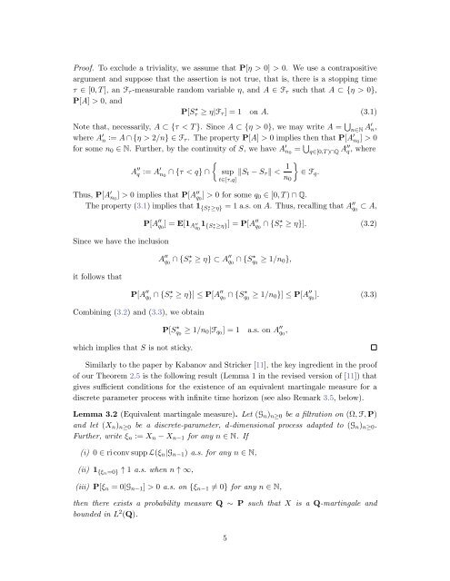
Proof. To exclude a triviality, we assume that P[η > 0] > 0. We use a contrapositive
argument and suppose that the assertion is not true, that is, there is a stopping time
τ ∈ [0, T ], an F τ -measurable random variable η, and A ∈ F τ such that A ⊂ {η > 0},
P[A] > 0, and
P[S ⋆ τ ≥ η|F τ ] = 1 on A. (3.1)
Note that, necessarily, A ⊂ {τ < T }. Since A ⊂ {η > 0}, we may write A = ⋃ n∈N A′ n,
where A ′ n := A ∩ {η > 2/n} ∈ F τ . The property P[A] > 0 implies then that P[A ′ n 0
] > 0
for some n 0 ∈ N. Further, by the continuity of S, we have A ′ n 0
= ⋃ q∈[0,T )∩Q A′′ q, where
{
A ′′
q := A′ n 0
∩ {τ < q} ∩
sup ‖S t − S τ ‖ < 1 }
∈ F q .
t∈[τ,q]
n 0
Thus, P[A ′ n 0
] > 0 implies that P[A ′′
q 0
] > 0 for some q 0 ∈ [0, T ) ∩ Q.
The property (3.1) implies that 1 {S ⋆ τ ≥η} = 1 a.s. on A. Thus, recalling that A ′′
q 0
⊂ A,
Since we have the inclusion
it follows that
P[A ′′
q 0
] = E[1 A ′′
q 0
1 {S ⋆ τ ≥η}] = P[A ′′
q 0
∩ {S ⋆ τ ≥ η}]. (3.2)
A ′′
q 0
∩ {S ⋆ τ ≥ η} ⊂ A ′′
q 0
∩ {S ⋆ q 0
≥ 1/n 0 },
P[A ′′
q 0
∩ {S ⋆ τ ≥ η}] ≤ P[A ′′
q 0
∩ {S ⋆ q 0
≥ 1/n 0 }] ≤ P[A ′′
q 0
]. (3.3)
Combining (3.2) and (3.3), we obtain
which implies that S is not sticky.
P[S ⋆ q 0
≥ 1/n 0 |F q0 ] = 1 a.s. on A ′′
q 0
,
Similarly to the paper by Kabanov and Stricker [11], the key ingredient in the proof
of our Theorem 2.5 is the following result (Lemma 1 in the revised version of [11]) that
gives sufficient conditions for the existence of an equivalent martingale measure for a
discrete parameter process with infinite time horizon (see also Remark 3.5, below).
Lemma 3.2 (Equivalent martingale measure). Let (G n ) n≥0 be a filtration on (Ω, F, P)
and let (X n ) n≥0 be a discrete-parameter, d-dimensional process adapted to (G n ) n≥0 .
Further, write ξ n := X n − X n−1 for any n ∈ N. If
(i) 0 ∈ ri conv supp L(ξ n |G n−1 ) a.s. for any n ∈ N,
(ii) 1 {ξn=0} ↑ 1 a.s. when n ↑ ∞,
(iii) P[ξ n = 0|G n−1 ] > 0 a.s. on {ξ n−1 ≠ 0} for any n ∈ N,
then there exists a probability measure Q ∼ P such that X is a Q-martingale and
bounded in L 2 (Q).
5