Decision Trees from large Databases: SLIQ

Decision Trees from large Databases: 

SLIQ 

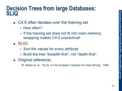
• C4.5 often iterates over the training set 

How often? 

If the training set does not fit into main memory, 

swapping makes C4.5 unpractical! 

• SLIQ: 

Sort the values for every attribute 

Build the tree “breadth-first“, not “depth-first“. 

• Original reference: 

M. Mehta et. al.: ”SLIQ: A Fast Scalable Classifier for Data Mining”. 1996 

Sawade/Landwehr/Prasse/Scheffer, Maschinelles Lernen 

41

SLIQ: Gini Index 

• To determine the best split, SLIQ uses the Gini- 

Index instead of Information Gain. 

• For a training set L with n distinct classes: 

Gini L = 1 − p j 

2 

j=1…n 

p j is the relative frequency of value j 

• After a binary split of the set L into sets L 1 and L 2 

the index becomes: 

Gini split L = L 1 

L Gini L 1 + L 2 

L Gini L 2 

• Gini-Index behaves similarly to Information Gain. 


42

Compare: Information Gain vs. Gini Index 

• Which split is better? 

[29 +, 35 -] 

yes 

x 1 

x 2 

no 

• H L, y = − 29 

64 log 2 29 

64 + 35 

64 log 2 35 

64 

= 0.99 

[29 +, 35 -] 

[21+, 5 -] [8+, 30 -] [18+, 33 -] [11+, 2 -] 

• IG L, x 1 = 0.99 − 26 

64 H L x 1 =yes, y + 38 

64 H L x 1 =no, y ≈ 0.26 

• IG L, x 2 = 0.99 − 51 

64 H L x 2 =yes, y + 13 

64 H L x 2 =no, y ≈ 0.11 

1 − 8 38 

• Gini x1 L = 26 

64 Gini L x 1 =yes + 38 

64 Gini L x 1 =no ≈ 0.32 

• Gini x2 L = 51 

64 Gini L x 2 =yes + 13 

64 Gini L x 2 =no ≈ 0.42 

43 

yes 

2 

+ 

30 

38 

2 

no 

≈ 0.33 

Sawade/Landwehr/Prasse/Scheffer, Maschinelles Lernen

SLIQ – Algorithm 

1. Start Pre-sorting of the samples. 

2. As long as the stop criterion has not been reached 

1. For every attribute 

1. Place all nodes into a class histogram. 

2. Start evaluation of the splits. 

2. Choose a split. 

3. Update the decision tree; for each new node 

update its class list (nodes). 


44

SLIQ (1st Substep) 

• Pre-sorting of the samples: 

1. For each attribute: create an attribute list with 

columns for the value, sample-ID and class. 

2. Create a class list with columns for the sample-ID, 

class and leaf node. 

3. Iterate over all training samples: 

 

For each attribute 

 

 

Insert its attribute values, sample-ID and class (sorted 

by attribute value) into the attribute list. 

Insert the sample-ID, the class and the leaf node 

(sorted by sample-ID) into the class list. 


45

SLIQ: Example 


46



47








 




48

SLIQ (2nd Substep) 

• Evaluation of the splits. 

1. For each node, and for all attributes 

1. Construct a histogram (for each class the histogram 

saves the count of samples before and after the 

split). 

2. For each attribute A 

1. For each value v (traverse the attribute list for A) 

1. Find the entry in the class list (provides the class and 

node). 

2. Update the histogram for the node. 

3. Assess the split (if its a maximum, record it!) 


49



50








 

 




51

SLIQ (3rd Substep) 

• Update the Class list (nodes). 

1. Traverse the attribute list of the attribute used in 

the node. 

2. For each entry (value, ID) 

3. Find the matching entry (ID, class, node) in the 

class list. 

4. Apply the split criterion emitting a new node. 

5. Replace the corresponding class list entry with (ID, 

class, new node). 


52



53

SLIQ: Data Structures 

• Data structures in memory? 

• Swappable data structures? 

• Data structures in a database? 


54

SLIQ- Pruning 

• Minimum Description Length (MDL): the best model 

for a given data set minimizes the sum of the length 

the encoded data by the model plus the length of 

the model. 

cost M, D = cost D M + cost M 

• cost M = cost of the model (length). 

How large is the decision tree? 

• cost D M = cost to describe the data with the 

model. 

How many classification errors are incurred? 


55

Pruning – MDL Example I 

• Assume: 16 binary attributes and 3 classes 

• cost M, D = cost D M + cost M 

Cost for the encoding of an internal node: 

log 2 (m) = log 2 16 = 4 

Cost for the encoding of a leaf: 

log 2 (k) = log 2 (3) = 2 

Cost for the encoding of a classification error for n 

training data points: 

log 2 (n) 

7 Errors 

C 1 

C 2 

C 3 


56

Pruning – MDL Example II 

• Which tree is better? 

7 Errors 

Tree 1: Tree 2: 

C 1 

C 1 

C 2 C 3 

Internal nodes Leaves Errors 

4 Errors 

C 2 

C 1 C 2 

• Cost for tree 1: 2 ∗ 4 + 3 ∗ 2 + 7 ∗ log 2 n = 14 + 7 log 2 n 

• Cost for tree 2: 4 ∗ 4 + 5 ∗ 2 + 4 ∗ log 2 n = 26 + 4 log 2 n 

• If n < 16, then tree 1 is better. 

• If n > 16, then tree 2 is better. 

C 3 


57

SLIQ – Properties 

• Running time for the initialization (pre-sorting): 

O n log n for each attribute 

• Much of the data must not be kept in main memory. 

• Good scalability. 

If the class list does not fit in main memory then SLIQ 

no longer works. 

Alternative: SPRINT 

• Can handle numerical and discrete attributes. 

• Parallelization of the process is possible. 


58

Regression Trees 

• ID3, C4.5, SLIQ: Solve classification problems. 

Goal: low error rate + small tree 

• Attribute can be continuous (except for ID3), but 

their prediction is discrete. 

• Regression: the prediction is continuously valued. 

Goal: low quadratic error rate + simple model. 

n 

2 

SSE = j=1 y j − f x j 

• Methods we will now examine: 

Regression trees, 

Linear Regression, 

Model trees. 


59


• Input: L = x 1 , y 1 , … , x n , y n , continuous y. 

• Desired result: f: X → Y 

• Algorithm CART 

It was developed simultaneously & independently 

from C4.5. 

Terminal nodes incorporate continuous values. 

Algorithm like C4.5. For classification, there are 

slightly different criteria (Gini instead of IG), but 

otherwise little difference. 

Information Gain (& Gini) only work for classification. 

Question: What is a split criterion for Regression? 


L. Breiman et. al.: ”Classification and Regression Trees”. 1984 


60


• Goal: small quadratic error (SSE) + small tree. 

• Examples L arrive at the current node. 

• SSE at the current node: SSE L = x,y ∈L y − y 2 

where y = 1 y 

L x,y ∈L . 

• With which test should the data be split? 

• Criterion for test nodes x ≤ v : 

SSE − Red L, x ≤ v = SSE L − SSE L x≤v − SSE L x>v 

SSE-Reduction through the test. 

• Stop Criterion: 

Do not make a new split unless the SSE will be 

reduced by at least some minimum threshold. 


If so, then create a terminal node with mean m of L. 

61

CART- Example 

• Which split is better? 

L = [2,3,4,10,11,12] 

SSE L = 100 

ja 

nein 

SSE L = y − y 2 

x,y ∈L where y = 1 L 

x 1 

x 2 

L = [2,3,4,10,11,12] 

ja 

nein 

L 1 = [2,3] L 2 =[4,10,11,12] L 1 =[2,4,10] L 2 =[3,11,12] 

SSE L 1 = 0,5 SSE L 2 = 38,75 SSE L 1 = 34,67 SSE L 2 = 48,67 

x,y ∈L 

y 


62

Linear Regression 

• Regression trees: constant prediction at every leaf 

node. 

• Linear Regression: Global model of a linear 

dependence between x and y. 

• Standard method. 

• Useful by itself and it serves as a building block for 

Model trees. 


63

Linear Regression 

• Input: L = x 1 , y 1 , … , x n , y n 

• Desired result: a linear model, f x = w T x + c 

Normal vector 

Residuals 

Points along the 

Regression line 

are perpendicular 

to the normal vector. 


64

Model Trees 

• Decision trees but with a linear regression model at 

each leaf node. 


.2 .3 .4 .5 .6 .7 .8 .9 1.0 1.1 1.2 1.3 

65

Model Trees 

• Decision trees but with a linear regression model at 

each leaf node. 

yes ja 

yes ja 

x < .9 

x < .5 x < 1.1 

no nein 

yes 

no nein 

nein no 


.1 .2 .3 .4 .5 .6 .7 .8 .9 1.0 1.1 1.2 1.3 

66

Model Trees: Creation of new Test Nodes 

• Fit a linear regression of all samples that are filtered 

to the current node. 

• Compute the regression‘s SSE. 

• Iterate over all possible tests (like C4.5): 

Fit a linear regression for the subset of samples on 

the left branch, & compute SSE left . 

Fit a linear regression for the subset of samples on 

the right branch, & compute SSE right . 

• Choose the test with the largest reduction 

SSE − SSE left − SSE right . 

• Stop-Criterion: If the SSE is not reduced by at least 

a minimum threshold, don‘t create a new test. 


67

Missing Attribute Values 

• Problem: Training data with missing attributes. 

• What if we test an attribute A for which an attribute 

value does not exist for every sample? 

These training samples receive a substitute attribute 

value which occurs most frequently for A among the 

samples at node n. 

These training samples receive a substitute attribute 

value, which most samples with the same 

classification have. 


68

Attributes with Costs 

• Example: Medical diagnosis 

A blood test costs more than taking one‘s pulse 

• Question: How can you learn a tree that is 

consistent with the training data at a low cost? 

• Solution: Replace Information Gain with: 

Tan and Schlimmer (1990): 

Nunez (1988): 

IG 2 L,x 

Cost A 

2 IG L,x −1 

Cost A +1 w 

Parameter w ∈ 0,1 controls the impact of the cost. 


69

Bootstrapping 

• Simple resampling method. 

• Generates many variants of a training set L. 

• Bootstrap Algorithm: 

Repeat k = 1 … M times: 

Generate a sample dataset L k of size n from L: 

• The sampled dataset is drawn uniformly with 

replacement from the original set of samples. 

Compute model θ k for dataset L k 

Return the parameters generated by the bootstrap: 

θ ∗ = 

θ 1 , … , θ M 


70

Bootstrapping - Example 

x = 

3.12 

0 

1.57 

19.67 

0.22 

2.20 

, x = 4,46 

x = 

x = 

x = 

1.57 

0.22 

19.67 

0 

0.22 

3.12 

0 

2.20 

19.67 

2.20 

2.20 

1.57 

0.22 

3.12 

1.57 

3.12 

2.20 

0.22 

, x = 4,13 

, x = 4,64 

, x = 1,74 

71 

Sawade/Landwehr/Prasse/Scheffer, Maschinelles Lernen

Bagging – Learning Robust Trees 

• Bagging = Bootstrap aggregating 

• Bagging – Algorithm: 

Repeat k = 1 … M times : 

Generate a sample dataset L k from L. 

Compute model θ k for dataset L k . 

• Combine the M learned predictive models: 

Classification problems: Voting 

Regression problems: Mean value 


L.Breiman: “Bagging Predictors”. 1996 

e.g. a model tree 


72

Random Forests 

• Repeat: 

Draw randomly n samples, uniformly with 

replacement, from the training set. 

Randomly select m ′ < m features 

Learn decision tree (without pruning) 

• Classification: Maximum over all trees (Voting) 

• Regression: Average over all trees 


L. Breiman: ”Random Forests”. 2001 

Bootstrap 


73

Usages of Decision Trees 

• Medical Diagnosis. 

• In face recognition. 

• As part of more complex systems. 


74

Decision Tree - Advantages 

• Easy to interpret. 

• Can be efficiently learned from many samples. 

SLIQ, SPRINT 

• Many Applications. 

• High Accuracy. 


75

Decision Tree - Disadvantages 

• Not robust against noise 

• Tendency to overfit 

• Unstable 


76

Summary of Decision Trees 

• Classification: Prediction of discrete values. 

Discrete attributes: ID3. 

Continuous attributes: C4.5. 

Scalable to large databases: SLIQ, SPRINT. 

• Regression: Prediction of continuous values. 

Regression trees: constant value predicted at each 

leaf. 

Model trees: a linear model is contained in each leaf. 


77

Decision Trees from large Databases: SLIQ

You also want an ePaper? Increase the reach of your titles

Delete template?

Save as template?