The Adaptive Radix Tree: ARTful Indexing for Main-Memory ...
The Adaptive Radix Tree: ARTful Indexing for Main-Memory ...
The Adaptive Radix Tree: ARTful Indexing for Main-Memory ...

Create successful ePaper yourself
Turn your PDF publications into a flip-book with our unique Google optimized e-Paper software.
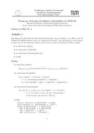
Fig. 4.<br />
Illustration of a radix tree using array nodes (left) and our adaptive radix tree ART (right).<br />
idea and shows that adaptive nodes do not affect the structure<br />
(i.e., height) of the tree, only the sizes of the nodes. By<br />
reducing space consumption, adaptive nodes allow to use a<br />
larger span and there<strong>for</strong>e increase per<strong>for</strong>mance too.<br />
In order to efficiently support incremental updates, it is<br />
too expensive to resize nodes after each update. <strong>The</strong>re<strong>for</strong>e,<br />
we use a small number of node types, each with a different<br />
fanout. Depending on the number of non-null children, the<br />
appropriate node type is used. When the capacity of a node<br />
is exhausted due to insertion, it is replaced by a larger node<br />
type. Correspondingly, when a node becomes underfull due to<br />
key removal, it is replaced by a smaller node type.<br />
C. Structure of Inner Nodes<br />
Conceptually, inner nodes map partial keys to child pointers.<br />
Internally, we use four data structures with different capacities.<br />
Given the next key byte, each data structure allows to efficiently<br />
find, add, and remove a child node. Additionally, the<br />
child pointers can be scanned in sorted order, which allows to<br />
implement range scans. We use a span of 8 bits, corresponding<br />
to partial keys of 1 byte and resulting a relatively large<br />
fanout. This choice also has the advantage of simplifying the<br />
implementation, because bytes are directly addressable which<br />
avoids bit shifting and masking operations.<br />
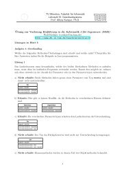
<strong>The</strong> four node types are illustrated in Figure 5 and are<br />
named according to their maximum capacity. Instead of using<br />
a list of key/value pairs, we split the list into one key part<br />
and one pointer part. This allows to keep the representation<br />
compact while permitting efficient search:<br />
Node4: <strong>The</strong> smallest node type can store up to 4 child<br />
pointers and uses an array of length 4 <strong>for</strong> keys and another<br />
array of the same length <strong>for</strong> pointers. <strong>The</strong> keys and pointers<br />
are stored at corresponding positions and the keys are sorted.<br />
Node16: This node type is used <strong>for</strong> storing between 5 and<br />
16 child pointers. Like the Node4, the keys and pointers<br />
are stored in separate arrays at corresponding positions, but<br />
both arrays have space <strong>for</strong> 16 entries. A key can be found<br />
efficiently with binary search or, on modern hardware, with<br />
parallel comparisons using SIMD instructions.<br />
Node48: As the number of entries in a node increases,<br />
searching the key array becomes expensive. <strong>The</strong>re<strong>for</strong>e, nodes<br />
with more than 16 pointers do not store the keys explicitly.<br />
Instead, a 256-element array is used, which can be indexed<br />
with key bytes directly. If a node has between 17 and 48 child<br />
pointers, this array stores indexes into a second array which<br />
contains up to 48 pointers. This indirection saves space in<br />
Node4<br />
Node16<br />
Node48<br />
Node256<br />
key<br />
0 2 3<br />
key<br />
child pointer<br />
child pointer<br />
0 1 2 15 0 1 2 15<br />
0 2 3 … 255<br />
…<br />
0 1 2<br />
child index<br />
0 1 2<br />
a<br />
0 1 2 3 0 1 2 3<br />
3 255<br />
…<br />
b<br />
255<br />
b<br />
child pointer<br />
c<br />
child pointer<br />
3 4 5 6 255<br />
…<br />
c<br />
a<br />
a<br />
0<br />
b<br />
Fig. 5. Data structures <strong>for</strong> inner nodes. In each case the partial keys 0, 2,<br />
3, and 255 are mapped to the subtrees a, b, c, and d, respectively.<br />
comparison to 256 pointers of 8 bytes, because the indexes<br />
only require 6 bits (we use 1 byte <strong>for</strong> simplicity).<br />
Node256: <strong>The</strong> largest node type is simply an array of 256<br />
pointers and is used <strong>for</strong> storing between 49 and 256 entries.<br />
With this representation, the next node can be found very<br />
efficiently using a single lookup of the key byte in that array.<br />
No additional indirection is necessary. If most entries are not<br />
null, this representation is also very space efficient because<br />
only pointers need to be stored.<br />
Additionally, at the front of each inner node, a header of<br />
constant size (e.g., 16 bytes) stores the node type, the number<br />
of children, and the compressed path (cf. Section III-E).<br />
D. Structure of Leaf Nodes<br />
Besides storing paths using the inner nodes as discussed<br />
in the previous section, radix trees must also store the values<br />
associated with the keys. We assume that only unique keys<br />
are stored, because non-unique indexes can be implemented<br />
by appending the tuple identifier to each key as a tie-breaker.<br />
<strong>The</strong> values can be stored in different ways:<br />
b<br />
1<br />
a<br />
c<br />
2<br />
c<br />
d<br />
…<br />
d<br />
47<br />
d<br />
d