Read Jillian's article (pdf) - Aquinas College

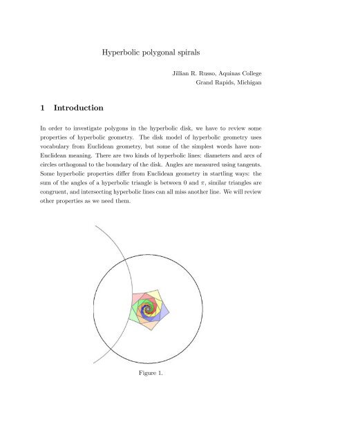
Hyperbolic polygonal spirals 

Jillian R. Russo, Aquinas College 

Grand Rapids, Michigan 

1 Introduction 

In order to investigate polygons in the hyperbolic disk, we have to review some 

properties of hyperbolic geometry. The disk model of hyperbolic geometry uses 

vocabulary from Euclidean geometry, but some of the simplest words have non- 

Euclidean meaning. There are two kinds of hyperbolic lines: diameters and arcs of 

circles orthogonal to the boundary of the disk. Angles are measured using tangents. 

Some hyperbolic properties di¤er from Euclidean geometry in startling ways: the 

sum of the angles of a hyperbolic triangle is between 0 and , similar triangles are 

congruent, and intersecting hyperbolic lines can all miss another line. We will review 

other properties as we need them. 

Figure 1.

Russo and McDaniel 2 

Figure 1 illustrates the topics in this article. The dark, complete circle is the 

boundary of our hyperbolic disk. The large arc which passes through this disk is 

part of a circle orthogonal to the disk. The intricate design is made of hyperbolic 

pentagons. The outermost pentagon is made of …ve hyperbolic segments which meet 

at right angles. The sides are made of arcs which lie in hyperbolic lines. To keep 

the drawing simple, we have drawn only one hyperbolic line in its entirety. 

Any nested pentagon has the midpoints of the sides of the previous pentagon 

for vertices. (We give instructions for the construction of this …gure in the third 

section.) The nested pentagons form hyperbolic triangles; we will …nd properties 

of one triangle from each level. The shading is to emphasize choosing one triangle 

from each level. 

A few more hyperbolic geometry facts we will use without proof: 

We can have a hyperbolic polygon with all right angles and as many sides as 

we want, as long as we want more than four. 

The nested polygons have a limiting case as they are constructed inward: the 

Euclidean regular polygon of that many sides. The hyperbolic segments get 

straighter as the polygons get smaller. 

As the polygons go inward, the hyperbolic length of a side approaches zero. 

The vertex angles grow from 2 

to the Euclidean limit. 

The nested polygons are not congruent and do not form a tiling. The initial 

vertex angles do not have to be ; they could be any size less than the Euclidean 

2 

value of n 2 

n 

, where n 5: 

2 Hyperbolic Trigonometry 

The hyperbolic disk has its own trigonometry, using sinh x and cosh x. We only need 

two hyperbolic identities, available in any hyperbolic trigonometry text [Kennelly]. 

We use triangle ABC whose sides are hyperbolic segments with hyperbolic lengths 

a; b; c.


A 

c 

B 

b 

a 

C 

Figure 2. Hyperbolic triangle ABC. 

cosh c = cosh a cosh b 

sinh a sinh b cos C 

The equation above resembles the Law of Cosines in that the only angle involved 

corresponds with the isolated side on the left hand of the equation. Since the formula 

uses cosh a instead of the hyperbolic length a, we will use cosh a in our calculations 

much more than a, even though we will investigate the hyperbolic lengths of the 

sides of our nested polygons. 

We will also use the special structure of our polygons to simplify the second 

useful identity. 

O 

F 

A 

B 

D 

E 

C 

Figure 3. Level k sketch. 

sin \OF D sin \ODF cosh F D = cos \DOF + cos \OF D cos \ODF 

The speci…c triangle OF D has speci…c values so that we can simplify quickly. 

We will take segment BD as length L k , making \ODF = A k 

2 . Since \OF D = 2 ; 

the formula becomes 

sin A k 

2 cosh L k 

2 = cos n :


With these formulas, we calculated angles, areas, and lengths for as many levels 

as we wanted. We used cosh L k = S k for all our calculations and notes and converted 

to hyperbolic length only when we wanted actual hyperbolic lengths. Our empirical 

investigation pointed the way to the theoretical results in this paper. 

3 Nested Hyperbolic Polygons 

We will now construct a regular hyperbolic pentagon with all right angles. In the 

hyperbolic disk, we can have regular polygons with the same number of sides but 

di¤erent angle sizes, as long as the angle size is less than the Euclidean size for 

a regular polygon.. This means,when we begin to imagine a sequence of nested 

polygons, we have to specify the size of angle and the number of sides we use at the 

…rst level. 

We will now construct a regular, right angled hyperbolic polygon and create 

layers of polygons inside it using the midpoints of the sides. The construction is 

simple (provided the initial angle is constructible) and can be done with a series of 

Euclidean moves using a compass and straight edge. 

Regular Right Angled Hyperbolic Polygon Construction 

B 

J 

A 

J 

H 

I 

A 

G 

B 

C 

E 

F 

D 

J 

H 

I 

B 

A C 

O 

E 

G 

F 

D 

H 

I 

C 

O 

E 

G 

F 

D 

Figure 4. 

Figure 5. Boundary location. 

Figure 6. Polygon construction. 

Start with the formula ( 

180(n 2) 

n 

).


180(n 2) 

Create a line AB of any length R. Rotate the line by the angle ( 

n 

) 

around point B with length R, creating line BC. 

Now rotate the line a negative 90 degrees around point C with length R, 

creating line CD. 

 

Continue the …rst two steps repeatedly, rotating around the newest created 

endpoint, until the sides close in on each other. (Figure 4) 

Connect the vertices at the angles of measure ( 

n-sided polygon with interior angles ( 

180(n 2) 

n 

). 

180(n 2) 

n 

), it will create an 

 

Connect two vertices of the n-sided polygon, skipping one in between. 

Construct the …rst side of the hyperbolic regular polygon. Use a vertex of 

the n-sided polygon as the center. Use radius of length R, so the hyperbolic line 

will go through the two points of length R away from the chosen vertex . 

Now construct the diagonals of the n-sided polygon to …nd the center. 

(Figure 5) 

The center of the hyperbolic space will be the center of the n-sided polygon 

(O), where all the diagonals meet. To …nd the radius follow the line we connected 

between two vertices (skipping one), starting at one of the vertices and traveling 

toward the other until we hit the hyperbolic line. 

Finish the polygon by creating the hyperbolic lines as before. Use the 

vertices of the n-sided polygon with radii of length R. (Figure 6) 

To make the …rst nested polygon start by creating lines perpendicular to 

the diagonals at all the vertices of the n-sided polygon. The intersections of these 

perpendicular lines create a new n-sided polygon. (Figure 7 - Pentagon MNPRS) 

Note: The midpoints of the arcs of the hyperbolic lines are the points where the 

diagonals intersect the arcs. 

Use the vertices of the newly created n-sided polygon as the center of the 

circles for the sides of the nested hyperbolic polygon. The radius will be the length 

from the vertices to the midpoint of the arc of one of the circles containing that 

point. (It will go through both midpoints). 

Repeat the last step for all vertices to …nish the …rst nested hyperbolic 

polygon.


 

Use the same three steps to construct multiple nested hyperbolic polygons 

always building o¤ the previous step. 

M 

B 

N 

J 

S 

I 

A 

G 

O 

C 

E 

D 

H 

F 

P 

R 

Figure 7. Nested polygon construction. 

These Euclidean steps make hyperbolic objects. We can see the circle with center 

J is orthogonal to the boundary circle with center O because a circle with diameter 

OJ has the two (unlabeled) points on Euclidean segment HB. We constructed the 

boundary circle for this to happen. 

We depend on these diagonals which skip one vertex, like HB, to …nd the centers 

of the circles which contain our hyperbolic lines. The Euclidean segment HB passes 

through the intersection of two circles and is called the radical axis of circles J 

and O. When one circle is a hyperbolic line and the other is the boundary, then


the radical axis contains the center of any hyperbolic line orthogonal to the given 

hyperbolic line (except the diameter, of course.) We have already built circles J and 

B orthogonal to the boundary. We can change our point of view and see that we 

have circle O orthogonal to circle B, treating circle B as the boundary, temporarily, 

of a hyperbolic disk. The two unlabeled points form a point and its inverse across 

circle B. We are relying on a property of orthogonal circles which can be found in 

[Goodman-Strauss], that a circle through a point and its inverse must be orthogonal 

to the circle of inversion. And, since circle J passes through these same two points, 

circle J must be orthogonal to circle B. This use of the radical axis is also given as 

a homework problem in [Venema]. 

3.0.1 The Area of One Spiral 

The shading in Figure 1 shows a spiral made from hyperbolic triangles, one from 

each level. The sum of the areas of these triangles is easily calculated. First, we 

need the area formula for a hyperbolic triangle ABC. With angles in radians, the 

area is (A + B + C). (There is a multiplication constant which we will take as 

1.) 

In Figure 1, we see n spirals all converging at O. Then the spirals …ll the interior 

of the …rst level polygon, with no overlap. For n sides, the spiral consists of 1 n of 

the area of the …rst level polygon. The hyperbolic area formula of the …rst level is 

(n 2) 

n 

2 = n 2 

2: 

We can divide by n to see the spiral has area 2 

A more interesting calculation can be made for this area, this time applying the 

hyperbolic area formula at each level and adding. We will get an honest-to-goodness 

telescopic series whose sum is, again, 2 

. A telescopic sum has terms which 

2 n 

cancel throughout the series, usually leaving a front term and a back term, as we will 

see in our example. We begin with a …gure of two consecutive levels in a polygon 

of n sides. 

2 

n .


G 

F 

A 

B 

β 

γ 

β 

δ 

D 

E 

C 

Figure 8. Supplementary angles at D. 

Using the area formula for a hyperbolic triangle again, we …nd the area of triangle 

BCD is 

( + 2) = ( + 2( ) 2) = : 

Now, these two angles and are just the vertex angles of isosceles hyperbolic 

triangles from two consecutive levels. The sum of the areas of hyperbolic triangles 

in the spiral would be a telescopic sum where the surviving terms would be the 

limit of the innermost angle minus the outermost angle. Luckily, both of these are 

available. The nested polygons approach a Euclidean regular polygon of n sides. 

The outermost angle is a right angle because we started with all right angles. We 

get the same area of the spiral: 

n 2 

n 

2 = 2 

2 

n : 

From this example, we see that we can …x the starter angle at size and the 

area of the spiral becomes 2 because the telescopic series will still happen. 

n 

If we use non-midpoints for the nested polygon vertices, we lose the nice isosceles 

structure. Yet, we keep the telescoping series! To see this in Figure 8, think of the 

two ’s as 1 and 2 . The calculation for the area of triangle BCD becomes 

( + 1 + 2 ) = + ( 1 2 )) = : 

The limit of the series is n 2 

n = 2 , the same answer as using midpoints. 

This makes sense because, even though we chose vertices o¤ the midpoints, 

n 

we still generate a spiral which stands for 1 n 

of the area inside the …rst polygon.


4 Sum of side lengths 

For hyperbolic triangle ABC, the hyperbolic trigonometric formula cosh c = cosh a cosh b 

sinh a sinh b cos C works nicely with our nested polygons. To translate into our levels, 

we use A k for the angle C. We will use L k for the hyperbolic length of one 

side at level k: More often, we will use S k = cosh L k . The isosceles structure of the 

triangle makes a = b = :5 cosh 1 (S k ). The side opposite angle A k already has a 

name: S k+1 . (The reason cosh 1 S k turns up so much is that S k is not hyperbolic 

length. We have to take cosh 1 S k to get hyperbolic length.) Substitution gives 

us our recursive formula for the hyperbolic length of a side of one of our nested 

hyperbolic polygons: 

S k+1 = [cosh 2 (:5 cosh 1 (S k )) (cos A k sinh 2 (:5 cosh 1 (S k ))]. 

Simpli…cations for the compositions cosh 2 (:5 cosh 1 (S k )) = S k + 1 

and sinh 2 (:5 cosh 1 (S k ) = 

2 

S k 1 

have been known since at least 1707 [Kennelly]. (The substitutions sinh 1 x = 

2 

ln(x + p x 2 + 1) and cosh 1 x = ln(x + p x 2 1) from any calculus text provide the 

key step.) The simpli…cations lead to a shorter recursive formula: 

S k+1 = 1 2 [S k(1 cos A k ) + (1 + cos A k )]: 

We are now ready to consider the sum of one side from each level. 

Claim: 

1X 

cosh 1 (S k ) < 1 for …xed M, the number of sides in the polygon: 

k=1 

Proof : Starting with the ratio test, we apply our recursive formula. Since all 

the subscripts have become k, we can suppress the subscripts. We are going to treat 

both S and A as functions of k. So, for example, S 0 = dS 

dk : 

cosh 1 (S k+1 ) cosh 1 ( 1 2 

lim 

k!1 cosh 1 = lim 

[S(1 cos A) + (1 + A)]) 

(S k ) k!1 

cosh 1 : 

(S) 

Since the limiting case is the center point O, we know the numerator and denominator 

go to 0. So we apply L’Hopital’s rule with k as the independent variable. 

k!1 

1 

lim 

k!1 

cos A) + (1 + A)]) 

cosh 1 ( 1 2 

lim 

[S(1 

cosh 1 (S) 

2 [S 0 (1 cos A) + (S 1)A 0 sin A] 

q 

S(1 cos A)+(1+A) 

[ 

2 

] 2 1 

= 

p 

S 2 1 

S 0 =


lim 

k!1 

p 

[S 0 (1 cos A) + (S 1)A 0 sin A] 

S 2 1 

p 

[S 2 (1 2 cos A + cos 2 A) + 2S(1 cos 2 A) + (1 + 2 cos A + cos 2 A)] 4 

lim 

k!1 

p 

[S 0 (1 cos A) + (S 1)A 0 sin A] 

S 2 1 

p 

[cos 2 A(S 1) 2 2 cos A(S 2 1) + (S + 3)(S 1) S 0 : 

S 0 = 

The lim S = 1; we see the factors of p S 1 cancel by division, so we can get 

k!1 

ready to take the limit. Before we can let the (S 1)A 0 sin A go to zero, however, 

we need to check that 

lim 

k!1 

A 0 sin A 

< 1. This is worth a look because the number S k approaches 1; so 

S 0 

S 0 can get small quickly. We will now make sure that A 0 gets small quickly enough 

to handle it. From our hyperbolic trigonometry formula for A = 2(sin 1 ( cos q 

n 

(subscripts suppressed), we …nd dA 

p 

2 cos( 

 

dS = 

n ) 

(S + 1) p S + 1 2 cos 2 ( by the Chain 

n 

) 

Rule. The lim S = 1 implies that this fraction is …nite for any …xed n. We can 

k!1 

…nish taking our limit. So the di¢ cult-looking factor A 0 sin A cancels in the limit 

and we …nd 

cosh 1 p 

(S k+1 ) 1 

lim 

k!1 cosh 1 = lim 

(S k ) k!1 

cos A 

p 

2 

< 1 for any …xed n. 

S+1 

2 

)) 

5 The constructible, regular, all right angled hyperbolic 

polygons 

Our constructions give us one more result. We can show that the family of constructible 

regular hyperbolic polygons is the same as the family of constructible 

Euclidean regular polygons. In this case, by "family," we mean the number of sides, 

more than four. If we can construct a regular n-sided Euclidean polygon, we can construct 

a regular, right angled hyperbolic polygon from it. We gave its construction 

at the start of Section 3. 

In order to show the families are the same, we just suppose we could construct 

a regular, n-sided, right angled hyperbolic polygon where n is not a power of 2 

times a product of distinct Fermat primes, like n = 7. In other words, suppose we 

have a construction for a regular, right angled, hyperbolic polygon whose Euclidean 

version is not in the constructible family. If this construction has O as its center, we 

can draw Euclidean segments connecting consecutive centers of circles containing


hyperbolic sides to construct a regular Euclidean polygon, which has been proved 

impossible. 

If this hyperbolic construction is o¤-center, the hyperbolic sides will not be 

congruent Euclidean arcs or segments. The centers of the circles containing these 

Euclidean arcs will not be spaced symmetrically around O. Steps exist, however, 

which will center the drawing, using compass and straightedge [Goodman-Strauss]. 

We can translate the o¤-center polygon to the location we use in this paper. Then 

we are right back to the previous paragraph, constructing an impossible Euclidean 

polygon. Therefore, our assumption that we can construct a regular, right angled 

hyperbolic polygon from outside the Euclidean family leads to a contradiction. 

Right angled hyperbolic polygons appear in the study of Riemann surfaces. As 

Castro and Martinez point out [Castro/Martinez], only a few papers exist which 

study these objects. The Euclidean versions of this problem have received more 

attention, in [Emmendorfer et al] and [Stewart]. 

Acknowledgment We thank the Dennison and Marguerite Mohler Fund for creating 

a summer research experience for my advisor, Dr. Michael McDaniel, and 

me. Dr. Aaron Cinzori’s talk on geometric spirals at our Math Club inspired our 

hyperbolic version. 

6 References 

A. E. Kennelly, The Application of Hyperbolic Functions to Electrical Engineering 

Problems, McGraw-Hill (1916). 

G. Venema, Foundations of Geometry, Prentice Hall (2005). 

C. Goodman-Strauss, Compass and straightedge in the Poincaré disk, The American 

Mathematical Monthly, 108, No. 1 (2001), 38 - 49. 

A. F. Costa and E. Martinez, On hyperbolic right-angled polygons, Geometricae 

Dedicata, 58, No. 3, (December 1995), 313 - 326. 

D. Emmendorfer, M. Precup, and A. Warren, Classi…cation of Geometric Spirals, 

Pi Mu Epsilon to appear. 

J. Stewart, Calculus, 6th edition, (Thomson) 799.

Read Jillian's article (pdf) - Aquinas College

You also want an ePaper? Increase the reach of your titles

Delete template?

Save as template?