Norm estimates for inverses of Vandermonde matrices

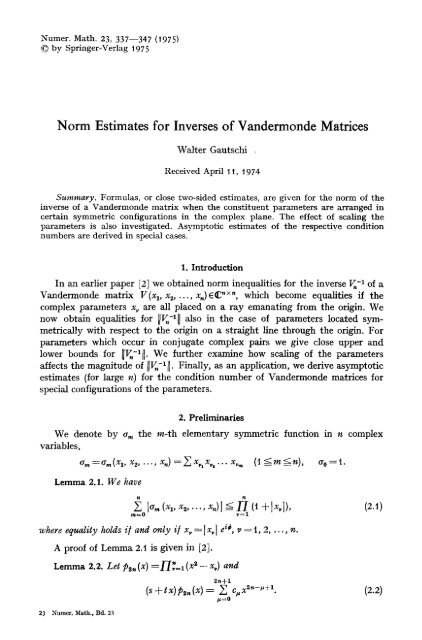
Numer. Math. 23, 337--347 (1975) 

9 by Springer-Verlag 1975 

Norm Estimates for Inverses of Vandermonde Matrices 

Walter Gautschi , 

Received April 11, 1974 

Summary. Formulas, or close two-sided estimates, are given for the norm of the 

inverse of a Vandermonde matrix when the constituent parameters are arranged in 

certain symmetric configurations in the complex plane. The effect of scaling the 

parameters is also investigated. Asymptotic estimates of the respective condition 

numbers are derived in special cases. 

1. Introduction 

In an earlier paper [21 we obtained norm inequalities for the inverse V~ -1 of a 

Vandermonde matrix V(x~, x~ ..... x,) E IE "• which become equalities if the 

complex parameters x~ are all placed on a ray emanating from the origin. We 

now obtain equalities for live-ill also in the case of parameters located symmetrically 

with respect to the origin on a straight line through the origin. For 

parameters which occur in conjugate complex pairs we give close upper and 

lower bounds for Ilv,-xl]. We further examine how scaling of the parameters 

affects the magnitude of llV,-lll. Finally, as an application, we derive asymptotic 

estimates (for large n) for the condition number of Vandermonde matrices for 

special configurations of the parameters. 

2. Preliminaries 

We denote by a,~ the m-th elementary symmetric function in n complex 

variables, 

a,~=am(xl, x2 ..... x~)= ~ x, x,..., x~ (1

338 W. Gautschi 

Then 

2.+1 

X le,,[ =

Norm Estimates for Inverses of Vandermonde Matrices 339 

For the coefficients cv in (2.5) we have 

c.=(--l)"(ta~--sa._~), 

where a-1 =a,.+~ =0. Therefore, 

/*=0, l ..... 2n+t, 

2n 2n+l 2n+l 2n 

Ilsl-Itll Y I~,,I ~ Y Ic.I-- X It~-s~.-,I _-__(Isl +1~1) X I~.1, 

/~=0 /*=0 /~=0 /*=0 

from which (2.6) follows by virtue of (2.8). 

3. Inversion of the Vandermonde Matrix 

We denote the Vandermonde matrix of order n by 

' 1 

| 

! I 

n--I n--i n--lt 

Lxl x2 ...x, _1 

where xx, x~ ..... x~ are distinct complex numbers and n > t. Its inverse can be 

obtained by solving the system of linear algebraic equations 

ul + us +.-. + u, =vl 

x~u~ + x, m +... + x~ u,=v~ (3.2) 

9 ..+x, 

u~=v,. 

Introducing the elementary Lagrange interpolation polynomials 

l~(x) = /~/ x,-xx-~x-xa ----a~nxn--l + a ",n--~ x n-~ +... +a~v v=l, 2 ..... n, (3.3) 

/*=i 

p4:v 

which satisfy 

l~(x,) = {10 

if v=/t 

if v4=t*, 

it is evident that by multiplying the/,-th Eq. (3-2) by a,v,/, = t, 2 ..... n, and 

adding, we get 

Consequently, 

u~,=~avuvt,, v---~l, 2, ..., n. 

[all 

al, ... aa,] 

23* 

La,,1 an2 ... a~] 

4. Norm Inequalities for V; t 

We consider throughout the oo-norm of V~ -1, 

IIv.-~ll~o =max 

l


Theorem 

Xl, x2, ..., x n. 

4.1. ][V-l(x~, x, ..... x,)[Ioo is a symmetric /unction in the variables 

Proo/. Interchanging two variables amounts to interchanging two columns 

of Vn, which in turn has the effect of interchanging two rows of V~ -1. The value 

of ]]V,-X[[| remains the same. 

Theorem 4.2. Let to 4=0 be arbitrary complex, and 

v, (o,) =~v(o, xl, ox~ ..... ~, x~). 

The. IIV;' (o)lL aepe~as only on 1~1 a~a is smctly decreasing as a/unction o~ I~l- 

Proo/. Let K =K(I), IT, -1 = [a,,]. Since 

we have V. -x (r 

V.(o~) =D(co)V~, D(r =diag(l, o) ..... 60"-1), 

=Vn-xn -1 (~o), i.e., 

~-~(o)=[ a,. 1 [ o~v-1 ]' v,l~=t,2 ..... n. 

It is clear, therefore, that the norm of V~ -1 (to) depends only on ]to]. Furthermore, 

if 1~11 O, v=l, 2 ..... n, 

in which case the equality in (4.t) can be given the alternative form 

where 

iiV-~ll~ = 

Ip.(-~)l 

min {(! +x,)IP;(*,)I} (x,>0), (4A') 

x


origin. In view of Theorem 4.2 we may assume the straight line to coincide with 

the real axis. 

Theorem 4.3. Let x, be distinct real numbers such that 

I/V~ = V(x 1, x, ..... x,), we then have 

x, + x,+l_ , = 0, v = t, 2 ..... n. (4.4) 

[! 2 max . {(t + !) *. v./i I"; l+x~ - d l } i! n is even, 

IV.-1L = (4.5) 

/max/~.(t + x.//-/i ,--~/. t + ~'~ i/.isoaa, 

I " t ~4, ix,-%lJ 

where v and p vary over all integers !or which x, >= 0 and x~, > O, respectively, and 

where e, = ~ when x, > O, and e, = 1 when x, = O. Alternatively, 

lie_, L = 

Ip.(01 t +x,* I}' (4.5') 

min, ( t~--~v Ipg(x,) 

where p~ ( x) is the polynomial in (4-3), and the minimum is taken over all nonnegative 

abscissas. 

Proo/. For the sake of definiteness we assume 

x,>0 for v=t, 2 ..... [n/2], x(,+l)/~=O if n is odd. (4.6) 

Let first n be even. The Lagrange polynomials (3.3) then are 

z,(x)- "+'./~''-~ l~§ v=1,2 ..... --~. 

/~4:v 

It suffices in (3.4) to evaluate the sums ~.~=~]a,,] for t _~, n/2) having the same values. An application of (3.3), (3.4) and Lemma 2.2, 

in which n is to be replaced by (n/2) --t, and s and t by 

1 t 

.12 

2 H (~:- d) 

hi2 

2 ~,, H (,~*.- ~,) 

$ - - ' ~ - - " 

la:4:t, 

then gives the first result in (4.5). The second, for n odd, is obtained similarly, 

noting that 

l, (~) , , l,,+~_.(~) =l.( - x), ~, = t, 2 .... - - 

X v 2X~ "~'j['l~l X v - - X~ ~ 2 ' 

t, eev 

(.--1)12 Xi -- X~ 

l(..)/~(x)= H (-d)" 

The alternative form (4.5') follows readily from (4.5) by observing that 

n/2 

p,(x) =H(x~-x~) 

p=1 

~eet' 

if n is even,


and 

(n - 1)/2 

p, (x) = x H ( x2 - x~) if n is odd. 

Corollary. I/n is even and x, are symmetric points as in (4.4), then (4.t) holds 

with strict inequality. 

Proo/. The bound in (4A), again assuming (4.6), is 

I ' ./2 (1 + x/*)~ 

max ,(t+~)/__/1 [x--~ x~ j, 

z l


Let 

5. Scaling of the Abscissas 

V.(co) = V(to xl, oJ x~ ..... to x.), to > 0. 

How does the norm of V~-l(to) compare with the norm of V,-X(l)? We shall 

answer this question first for positive abscissas x,, and then for symmetric real 

abscissas. 

Theorem 5.1. Let x, be distinct positive numbers. Then ]or to > O, 

o,+1 p.(-l) < Hv;'o)llo~ 

where p,(x) is the polynomial in (4.3). 

Proo[. From (4A') we obtain 


We need to show that 

2(~ - !) ~ + ! 

-~i 0 assumes the minimum value 2 (1/2 -- t) at y = V ~ - t. 

if t > 1, we use the first identity in (5.4) to obtain again 

go(O > 

i 2(1/~-1) _ 2(~-1) 

to 1 

--+t 

co+l 

co 

Combining the left inequality in (L3) just established with the second identity 

in (5.4) gives the right inequality, and thus proves (5.3). 

6. Examples 

Norm estimates for V~ -1 imply estimates for the condition number of V,. 

These in turn are of interest, e.g., in the study of the condition of polynomial 

interpolation [3]. In the examples which follow we derive asymptotic estimates 

for the condition number, assuming typical configurations of interpolation points. 

Example 6.1 (equidistant points), xv=t 2(v-l) n-I , v=l,2 .... ,n. We 

assume first n even. From (4.5) we find after some computation that 

where 

0s n 

V;1L - rain ~,' 

l


For n odd, we find similarly, 

sinh (r ~[n +1 . n--t~2 

V;q = z~(_~_t 7:1 .~ )! , "~ -t-~--~-} (n odd). (6.1o) 

Since 

condoo Vn = I1= =-I1 I1 , (6.2) 

using Stirling's formula for the gamma function, and straightforward, but 

tedious, manipulations, we find from (6.t) that 

1 _n n 1 

condoo V.,~ ~ e ~ e"(u +-~-'n*), n-+~. (6.3) 

Some numerical values x are listed in Table t. 

Table 1. Condition of polynomial interpolation at equidistant points on ~- 1, 1 ] 

n condo0 V n (6.3) 

5 5.0000 (1) 4.t668 (I) 

t0 1.3625 (4) t.1963 (4) 

20 1.0535 (9) 9.8614 (8) 

40 6.9269 (t8) 6.7007 (18) 

80 3.1456 (38) 3.0937 (38) 

2~-- 1 

Example 6.2 (Chebyshev points), x~ =cos 0~, 0, = 2n -~' v =1, 2 ..... n. 

The abscissas x, are the zeros of the Chebyshev polynomial of the first kind, 

T,~(x). Hence, by (4.5'), since [T'(x,) I =n/sin 0,, we find that 

where 

I1 - 11 - 

[ T~ (i)[ 

.. mini(0,) ' 

! +cos ~ 0 

1(0) = (t +cos 0) sin 0' o


it then follows that 

Consequently, by (6.4), 

min/(0,,,)-->/(0o) 

v 

33/4 

as n -+oo. 

/r ---> oo. 

On the other hand [4, p. 194], 

I Z,(r ~(l + lf2:, 

so that, in view of (6.2), 

3314 

cond| V~ ,~ ~- (l + ]/2)", 

Some numerical values are listed in Table 2. 

T/; -& oo 

n -+ oo. 

(6.5) 

Table 2. Condition of polynomial interpolation at Chebyshev points 

n condoo V n (6.5) 

5 4.1000 (t) 4.6737 (t) 

tO 3.7495 (3) 3.8330 (3) 

20 2.5727 (7) 2.578t (7) 

40 1.1663 (15) 1.1663 (t5) 

80 2.3859 (30) 2.3869 (30) 

Example 6.3. x,=t --e -i'~ v=t, 2 ..... n (even), h > O, 

0


Example 6.4 (Roots of unity), x, =e 2~i'/", v-----l, 2, ..., n. 

Although none of the previous estimates apply, we can obtain the inverse of 

the Vandermonde matrix directly by observing that the Lagrange interpolation 

polynomials are 

t,(x)=~- ~.~/ , ~=1,2 ..... n. 

Consequently, by (3.3), (%4), 

IIv/*u| =t, cond V ---n. 

Actually, the roots of unity are an optimal point configuration with regard 

to the spectral condition of Vandermonde matrices [3 ]. In fact, since V ff V~ = n 9 I,, 

we have cond2V ~ = t. 

References 

1. Bettis, D. G. : Numerical integration of products of Fourier and ordinary polynomials. 

Numer. Math. 14, 421-434 (1970) 

2. Gautschi, W. : On inverses of Vandermonde and confluent Vandermonde matrices. 

Numer. Math. 4, 117-123 (1962) 

3. Singhal, K., Vlach, J. : Accuracy and speed of real and complex interpolation. 

Computing 11, 147-158 (1973) 

4. Szeg6, G. : Orthogonal polynomials, 2nd rev. ed., Amer. Math. Soc. Colloq. Publ., 

Vol. 23, Amer. Math. Soc., Providence, R.I., 1959 

Prof. W. Gautschi 

Department of Computer Sciences 

Purdue University 

Lafayette, Indiana 47907~U.S.A.

Norm estimates for inverses of Vandermonde matrices

Create successful ePaper yourself

Delete template?

Save as template?