SAP2000 Dynamic Analysis - College of Engineering
SAP2000 Dynamic Analysis - College of Engineering
SAP2000 Dynamic Analysis - College of Engineering

Create successful ePaper yourself
Turn your PDF publications into a flip-book with our unique Google optimized e-Paper software.
Department <strong>of</strong> Civil & Geological <strong>Engineering</strong><br />
COLLEGE OF<br />
ENGINEERING<br />
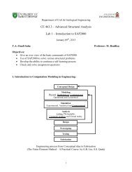
CE 463.3 – Advanced Structural <strong>Analysis</strong><br />
Lab 5 –<strong>SAP2000</strong> <strong>Dynamic</strong> <strong>Analysis</strong><br />
March 13 th , 2013<br />
T.A: Ouafi Saha<br />
Pr<strong>of</strong>essor: M. Boulfiza<br />
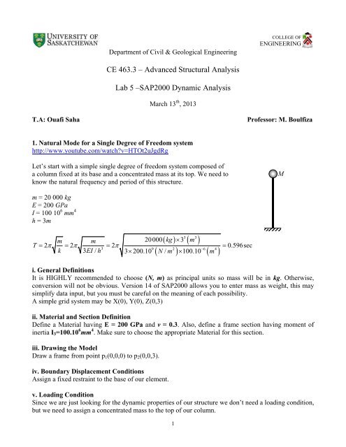
1. Natural Mode for a Single Degree <strong>of</strong> Freedom system<br />
http://www.youtube.com/watch?v=HTOt2uJgdRg<br />
Let’s start with a simple single degree <strong>of</strong> freedom system composed <strong>of</strong><br />
a column fixed at its base and a concentrated mass at its top. We need to<br />
know the natural frequency and period <strong>of</strong> this structure.<br />
M<br />
m = 20 000 kg<br />
E = 200 GPa<br />
I = 100 10 6 mm 4<br />
h = 3m<br />
T<br />
3 3<br />
kg<br />
<br />
m<br />
<br />
<br />
<br />
m m<br />
20000 3<br />
2 2 2 0.596sec<br />
3 9 2 6 4<br />
k 3 EI / h 3200.10 N / m 100.10 m<br />
i. General Definitions<br />
It is HIGHLY recommended to choose (N, m) as principal units so mass will be in kg. Otherwise,<br />
conversion will not be obvious. Version 14 <strong>of</strong> <strong>SAP2000</strong> allows you to enter mass as weight, this may<br />
simplify data input, but you must be careful on the meaning <strong>of</strong> each possibility.<br />
A simple grid system may be X(0), Y(0), Z(0,3)<br />
ii. Material and Section Definition<br />
Define a Material having E = 200 GPa and v = 0.3. Also, define a frame section having moment <strong>of</strong><br />
inertia I 3 =100.10 6 mm 4 . Make sure to choose the appropriate Material for this section.<br />
iii. Drawing the Model<br />
Draw a frame from point p 1 (0,0,0) to p 2 (0,0,3).<br />
iv. Boundary Displacement Conditions<br />
Assign a fixed restraint to the base <strong>of</strong> our element.<br />
v. Loading Condition<br />
Since we are just looking for the dynamic properties <strong>of</strong> our structure we don’t need a loading condition,<br />
but we need to assign a concentrated mass to the top <strong>of</strong> our column.<br />
1
Select the top node (joint)<br />
Assign > Joints > masses …<br />
Select Mass<br />
Mass in kg<br />
in local 1 axis<br />
N, m, sec<br />
lead to kg<br />
vi. Analyse the System<br />
Simplify analysis by choosing XZ Plane in “Set <strong>Analysis</strong> Options” menu<br />
Make sure to set MODAL to run in the “Run <strong>Analysis</strong>” dialogue box, no need to run Static analysis.<br />
Then Run the analysis.<br />
vii. Display Output<br />
An easy way to see the dynamic characteristics <strong>of</strong> the system is to use the tabular form output.<br />
Select Menu Display > Show Tables …<br />
2
viii. Discussing Results<br />
As we can see, the same period T = 0.596075sec as the hand calculated one is obtained. The natural<br />
frequency is f = 1.6776 Hz and the circular frequency is = 10.541 rad/sec<br />
3
2. Natural Mode for a Single Degree <strong>of</strong> Freedom one storey Building<br />
http://www.youtube.com/watch?v=O1rZRojOf4c<br />
Let’s study the structure shown in the next figure.<br />
M<br />
Assumptions:<br />
- Structure works in XZ plane.<br />
- All members are made <strong>of</strong> steel, E=200GPa.<br />
- All members’ self-weight is neglected.<br />
- The only existing mass is concentrated in the ro<strong>of</strong>.<br />
- Structure is fixed at its base.<br />
E, I c h<br />
E, I b l<br />
E, I c h<br />
Columns W310x74 (from CISC data base) I c = 165.10 6 mm 4<br />
h = 3m, l = 6m, M = 30 000kg.<br />
Ro<strong>of</strong> will be modeled in four different ways.<br />
Quick steps:<br />
- Choose N, m, C units<br />
- Define grids X(0,3,6) Y(0) Z(0,3)<br />
- Add new material Mat (E=200E9, v = 0.3, Self-weight=0)<br />
- Add section W310x74 by importing I/Wide flange from CISC database<br />
- Draw the frame using the same section for all parts<br />
- Fix foundation<br />
- Draw Special Joint at the middle <strong>of</strong> the ro<strong>of</strong><br />
- Assign concentrated mass to that joint = 30000 in local 1 st direction as mass. (§ expl. 1)<br />
- Only planar XZ degrees <strong>of</strong> Freedom are needed for this problem<br />
- No need for static analysis<br />
4
a. Ro<strong>of</strong> as Normal beam<br />
Just like we have already defined our structure<br />
In this case I b = I c<br />
The ro<strong>of</strong> is very flexible.<br />
T = 0.284162 sec<br />
f = 3.5191 Hz<br />
b. Use <strong>of</strong> Diaphragm<br />
Select all three top nodes then go to Menu Assign > Joints > Constraints …<br />
Select diaphragm in the first dialogue box and keep Z axis selected in the second dialogue box.<br />
This enforces the selected joints to maintain exactly the same distance from each other while moving in<br />
the XY plane.<br />
This constraint is usually used to model concrete<br />
slabs or decks.<br />
This does not lead to a big change in the example<br />
under consideration. The reason is that only the<br />
compression in the ro<strong>of</strong> beam has been<br />
constrained.<br />
T = 0.28251 sec<br />
f = 3.5397 Hz<br />
Alternatively, we can use the Equal Constraint.<br />
In this case choose all DOF to be equal. As we see<br />
from the figure, the structure is stiffer but this<br />
condition is not realistic.<br />
T = 0.243478 sec<br />
f = 4.1071 Hz<br />
5
c. Increase the stiffness <strong>of</strong> the ro<strong>of</strong> beam<br />
Remember to remove constraints before doing this step.<br />
Select the top beam then Menu Assign > Frame > Property Modifiers …<br />
In this case we are multiplying the flexural<br />
stiffness (Moment <strong>of</strong> Inertia I 3 ) <strong>of</strong> the top beam by<br />
a factor <strong>of</strong> 10.<br />
It’s clear that the top slab is almost horizontal.<br />
T = 0.234911 sec<br />
f = 4.2569 Hz<br />
d. No rotation in the top beam<br />
Remember to set the property modifiers to 1 again.<br />
Select the three nodes <strong>of</strong> the top and Assign > Joints > Restrains …<br />
This is the closest “realistic” condition to the use<br />
12EI<br />
<strong>of</strong> the formula k for column stiffness.<br />
3<br />
h<br />
T = 0.219775 sec<br />
f = 4.5501 Hz<br />
Why do you thik the above result is different<br />
from yours?<br />
Theoretical period calculated with formula above is T=0.2009sec. How can you find it with <strong>SAP2000</strong>?<br />
6
3. Multi Degrees <strong>of</strong> Freedom Building<br />
Consider the following 3 stories building<br />
To simplify, we assume:<br />
- All bays are 6m wide.<br />
- The first floor is 4m high and the other are in 3m spacing.<br />
- Self-weight <strong>of</strong> all elements is neglected.<br />
- Mass <strong>of</strong> each 6m segment slab is 25000 kg.<br />
- Slabs are considered infinitely rigid.<br />
- Moment <strong>of</strong> inertia <strong>of</strong> all columns, I c =150.10 6 mm 4 .<br />
- Material used is steel, E=200GPa, v = 0.3.<br />
E, I c h<br />
Find the three natural modes for horizontal displacement.<br />
Quick steps:<br />
- Choose N, m, C units (so we can use kg as unit for mass)<br />
- Use the predefined 2D Frame Model<br />
3 Stories @4m high<br />
3 Bays @6m width<br />
- Change grid lines Z (8, 12) to (7, 10) respectively, check on “glue joint to gridlines” before validating<br />
- Delete unwanted parts from the drawn model<br />
- Add new material MAT (E=200E9, v = 0.3, Self-weight=0)<br />
- Add section SEC as General where you put only I 3 =15E7mm, don’t forget to choose MAT as material<br />
- Select all structure elements and assign “SEC” to them<br />
- Fix foundation<br />
- Since we are restricting our structure to move only along the horizontal direction, position <strong>of</strong> the<br />
concentrated mass along X axis does not matter, as long as it is at the slab levels<br />
- Assign a resultant concentrated mass to each level: 25000 to the ro<strong>of</strong>, 50000 to the second floor and<br />
75000 to the first floor (my choice was to prescribe them along the second column)<br />
7
- Select all nodes above foundation and assign horizontal diaphragms to each level<br />
Horizontal<br />
Diaphragm<br />
Each level<br />
- Select all nodes above foundation and assign restrained rotation about local 2 nd axis<br />
- Only planar XZ degrees <strong>of</strong> Freedom are needed for this problem<br />
- Run the analysis with No static analysis<br />
T 1 =0.56032sec, T 2 =0.20508sec, T 3 =0.13491sec and f 1 =1.785Hz, f 2 =4.876Hz, f 3 =7.412Hz<br />
8
4. Two Degrees <strong>of</strong> Freedom System with Time History <strong>Analysis</strong><br />
http://www.youtube.com/watch?v=njWwO4hOwmI<br />
Let’s assume the simplified 2 DOF system shown below:<br />
- Self-weight <strong>of</strong> all elements is neglected.<br />
- Material used is steel E = 200 GPa, v = 0.3.<br />
- h = 3 m, M 1 = M 2 = 50000 kg, I 1 = I 2 = 450.10 6 mm 4<br />
- No rotations are allowed at the two levels (so we can use<br />
12EI<br />
k formula)<br />
3<br />
h<br />
Use modal analysis to find the two fundamental frequencies.<br />
In addition there is a harmonic concentrated load at the top level F(t).<br />
F(t)<br />
M 2<br />
E, I 2<br />
M 1<br />
E, I 1<br />
h<br />
h<br />
Solution:<br />
Modal <strong>Analysis</strong>:<br />
The first part will be done just like the first example. Two differences are however worth<br />
mentioning; we have two stories and rotation about local 2 nd axis is blocked.<br />
A first run will result in: T 1 =0.35944sec, f 1 =2.78213Hz, T 2 =0.13729sec, f 2 =7.28371Hz<br />
Time History <strong>Analysis</strong>:<br />
The second part needs more concentration!<br />
- Since we have the dynamic Concentrated Load at the top level, we need to add a concentrated static<br />
unit load in the Dead Load Case, even if we don’t need to run the static load <strong>Analysis</strong>.<br />
- Define the Harmonic function, Menu Define > Functions > Time History …<br />
In the first dialogue box choose Sine and click on Add New Function, in the second dialogue box<br />
change just the name <strong>of</strong> the function to SIN1, further functions can be generated later.<br />
9
- Define a new Load case for the Time History <strong>Analysis</strong>, Menu Define > Load Cases …<br />
Click on Add New Load Case … button<br />
Choose a<br />
name for the<br />
load case<br />
First choose<br />
Time History<br />
For Steady<br />
state choose<br />
Periodic<br />
Change Function<br />
to SIN1 and Scale<br />
factor to 1e7 then<br />
click on Add<br />
Change to<br />
finer time<br />
step<br />
Neglect the<br />
damping effect<br />
Scale Factor has been used because the unit dead load introduced previously (1N) is not big enough to<br />
move the system. (1E7 is a bit exaggerated).<br />
If you want to see the transient solution (starting from time t = 0 sec) click on Transient.<br />
It is highly recommended to use Time Step Data in accordance with Time History Function Definition,<br />
in this case SIN1, to avoid direct integration numerical perturbation.<br />
To neglect the effect <strong>of</strong> damping, click on Modify/Show… button under other parameter and put 0 for<br />
constant damping for all modes.<br />
Now Run! The analysis<br />
A good way to display the results for time history analysis is to use the built-in plot engine<br />
Menu Display > Show Plot Functions…<br />
10
We need first to define our probing stations. I have chosen the two horizontal displacements <strong>of</strong> the<br />
concentrated masses and the unit harmonic load.<br />
Click on Define Plot Functions…<br />
Define once for<br />
2 then for 3<br />
The final step is to add these three Plots to the vertical Functions side and click on Display<br />
11
Period <strong>of</strong> SIN1 = 1sec (Periodic)<br />
Period <strong>of</strong> SIN1 = 0.36sec (Transient)<br />
12
Period <strong>of</strong> SIN1 = 0.14sec (Transient)<br />
Period <strong>of</strong> SIN1 = 0.157sec (Periodic)<br />
Note that in the last run, Joint3 is still the node where the load is applied. But in this case it is not<br />
moving at all. Can you explain why?<br />
6. Additional Examples<br />
6.1. Find the fundamental period and frequency <strong>of</strong> the following beams with a lumped mass at<br />
midspan.<br />
Compare the results with hand calculated formula.<br />
m = 10 000 kg, E = 200 GPa, I = 150 10 6 mm 4 , l = 6m<br />
l/2<br />
M<br />
E,I<br />
l/2<br />
l/2<br />
M<br />
E,I<br />
l/2<br />
13
6.2. Repeat example 3 using the simplified model shown below, made <strong>of</strong> one vertical column, and three<br />
concentrated masses.<br />
M 3<br />
I 3<br />
M 2<br />
I 2<br />
M 1<br />
I 1<br />
6.3. Try to use the weight as masses and compare the results.<br />
14