Slides

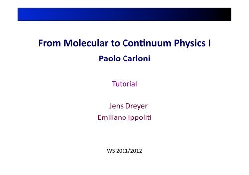
From Molecular to Con/nuum Physics I 

Paolo Carloni 

Tutorial 

Jens Dreyer 

Emiliano Ippoli4 

WS 2011/2012

RWTH Cluster 

• Connec4ng to the RWTH cluster: 

ssh –Y @cluster.rz.rwth-‐aachen.de 

• You need to be on the Aachen network: 

e.g. eduroam WLAN (Aachen or Jülich), RWTH VPN 

• Introduc4on to RWTH cluster 

• Users guide 

• Reference website 

• Tutorial files: /home/ei250498/TUTORIALS/ACETONE 

– Input files, COMMANDS, addi4onal necessary files , (output files) for each sec4on 

• Local course home page: 

/hbp://www.grs-‐sim.de/research/biophysics/courses/fmcp_tutorial.html

Car-Parinello / Molecular Mechanics 

• Introduc/on to “prac/cal” computa/onal chemistry / 

theore/cal biophysics 

• Setup and execu/on of calcula/ons 

• Interpreta/on of results 

• Example: Dipole moment of acetone 

– Gas phase 

– Environmental effects 

– Temperature effects

Geometry Optimization 

• Characteris4c points 

gradient = 0 

for all characteris4c points 

Minimum: 2 nd deriva4ves > 0 

Maximum: 2 nd deriva4ves < 0 

Transi4on state = first order saddle point: 

Single 2 nd deriva4ve < 0 (reac4on coordinate) 

All other 2 nd deriva4ves > 0 

Higher order saddle points: 

several 2 nd deriva4ves < 0 

other 2 nd deriva4ves > 0

Potential Energy Surfaces 

• Geometry op4miza4on 

• Minima 

• Transi4on states 

• Ac4va4on energies 

IR

Molecular Dipole Moments 

• Dipole moment defini/on: 

– Two iden4cal charges Q with a distance d 

-‐Q 

+Q 

– Convention 

• Physics, physical and theore4cal chemistry: 

• Engineering, organic/inorganic chemistry:


• Molecular dipole moments 

– k nuclei with charges +Z k • e: 

– Z e electrons with charges e: 

electronic 

distributions 

with arbitrary origin 

using pos. (S + ) and neg. (S -‐ ) centers 

of charges with S+ as origin 

Figures: W. Demtröder Experimentalphysik 2, Springer Verlag, Berlin, 2009.


• Molecular dipole moments 

– Examples 

H 2 O: 

4 pm 

Figures: W. Demtröder Experimentalphysik 2, 

Springer Verlag, Berlin, 2009.

Quantum Mechanical Dipole Moments

Dipole Moment and Symmetry 

Ψ 0 : allways totally symmetric for closed shell systems 

• The dipole moment can only be different from zero if one of its components, e.g. z (x, y, z) 

belongs to the to totally symmetric representa4on. 

• z can only belong to the totally symmetric representa4on if the point group (molecule) does 

not have a center of inversion nor a horizontal mirror plane (perpendicular to z). 

• Thus, only the point groups C 1 , C s , C n and C nv can have dipole moments different from zero.


Alignment of dipole molecules 

on charges 

Alignment in electric fields 

without field 

Coulomb interac4ons 

in salt crystals 

Alignment of dipole molecules 

in the solid state 

with field

Dipole Moment Convergence 

• Func4on of the level of theory 

aug = augmented 

(diffuse func4ons) are important 

GGA: worse than LSDA 

„exact exchange: improvement 

Tables: F. Jensen Introduc:on to Computa:onal Chemistry, Wiley VCH, Weinheim, 2007.

Dipole Moment Of Acetone 

• Procedure 

– Gas phase 

• Construct the molecular geometry, e.g. using MOLDEN in internal coordinates 

and export in cartesian coordinates. 

• Geometry op4miza4on using CPMD 

– Environmental and temperature effects 

• Classiscal MD simula4on of acetone in a water box (AMBER) 

• QM/MM (Car-‐Parinello – MD / GROMACS) hybrid simula4on

Cartesian Coordinates 

Rows of cartesian (xyz) 

coordinates 

C 0.000000 0.000000 0.000000 

H 0.000000 0.000000 1.089000 

H 1.029670 0.000000 -0.354544 

H -0.444367 0.973572 -0.201536 

H -0.555157 -0.777102 -0.523292

Internal Coordinates 

Bond lengths 

Bond angles 

Dihedral angle 

r (1-‐2) 

(3-‐1-‐2) 

(4-‐2-‐1-‐3) 

MOLDEN

Running Molden 

Ini4aliza4on: 

source /home/ei250498/PROGRAMS/modules/molden.sh 

Running: 

molden &

CPMD Input 

• General 

– Sec4ons: &NAME … &END 

– KEYWORDS in upper case, otherwise ignored 

– Sequence of sec4ons not important 

• Minimal input: 3 sec4ons 

– &CPMD … &END 

• Type of calcula4on: 

e.g. wave func4on op4miza4on, geometry op4miza4on, CPMD, … . 

– &SYSTEM … &END 

• System parameters: symmetry, cell, cutoff 

• Symmetry, shape and size of the simula4on cell 

– &ATOMS … &END 

• Atomic coordinates (cartesian) 

• Pseudopoten4als

CPMD Input 

• &CPMD … &END (required) 

– General control parameters for calcula4on, e.g. 

• Wavefunc4on op4miza4on (“single point calcula4on”) 

(default: 1.0D-‐5) 


„XYZ“ requests output files (in xyz-‐format): 

GEOMETRY.xyz : final (if converged: 

„op4mized“) structure 

OPT_GEO.xyz : op4miza4on trajectory

CPMD Input 

• &SYSTEM … &END (required) 

– Simula4on cell and plane wave parameters 

• In CPMD all calcula4ons are inherently periodic: 

For “gas phase” calcula4ons the cell has to be large enough to avoid significant 

interac4ons between periodic neighbours. 

in a.u. (1 bohr = 1 a 0 

= 0.529 Å ) 

a b/a c/a cos cos cos 

orthorhombic 

acetone box + 7 Å 

ABSOLUTE: a b c 

cos a cos b cos g 

cutoff for the plane wave in 

rydberg (size of basis set) 

1 Ry = 1/2 E h 

= 13.6 eV 

(binding energy of 1s electron in H atom

Plane Waves 

– Plane wave basis sets depend only on the size of the periodic cell, and not 

on the actual system to describe within the cell. 

– This is in contrast to the linear increase of Gaussian basis sets with 

system size, i.e. plane waves become more favourable for large systems. 

– Plane wave are primarily used for periodic systems, but can also be used 

for molecules in supercells, where the cell is sufficiently large to prevent 

self-‐interac4on with image cells. 

– Placing a small molecule into a large supercell requires many plane 

waves, which is more efficiently handled by localized Gaussian func4ons. 

– A 3D-‐periodic system, however, me be beber described by plane waves. 

– Plane waves 

• describe delocalized slowly varying electron densi4es very well (e.g. metals) 

• core electrons, however are strongly localized 

• valence electrons have many rapid oscilla4ons in the core region to maintain 

orthogonality 

• describing the core region adequately requires a large number of plane waves. 

– Thus, plane waves are used in connec4on with pseudopoten4als

Choosing the Plane Wave Cutoff 

• Convergence behavior 

rela4ve error 

(no systema4c errors included) 

MT = Mar4ns-‐Trouiller 

BHS =

CPMD Input 

• &DFT … &END (op4onal) 

– Exchange and correla4on func4onal 

• Default: LDA 

• Gradient-‐corrected func4onals 

• Hybrid func4onals

CPMD Input 

• &ATOMS … &END (required) 

– Pseudopoten4als and atomic coordinates 

*atom _file name of the pseudopoten4al 

number of atoms of the current type 

x y z 

... 

Label specifying the method how 

to calculate the nonlocal parts of 

the pseudopoten4al. 

... 

Informa4on on the nonlocality of the 

pseudopoten4al: 

LMAX=l with l being the maximum 

quantum number s,p,d.

Running CPMD 

To run the 64-‐bit version in CPMD-‐3.13.2 (with QMMM rou4nes) execute: 

source /home/ei250498/PROGRAMS/modules/cpmd.sh 

Calcula4on on one node: 

$MPIEXEC $FLAGS_MPI_BATCH /home/ei250498/PROGRAMS/BIN/cpmd.x 

/home/ei250498/PROGRAMS/SRC/cpmd/PP > 

Batch file 

#BSUB -J Template 

#BSUB -o output 

#BSUB -e error 

!Batch system’s job name! 

!Filename of the batch system’s output messages (and error if no option -e used)! 

!Filename of the batch system’s error messages! 

#BSUB -n 2 ! !Number of cores to be reserve for the job (for this tutorial use n < 8)! 

#BSUB -W 00:15 

!Hard runtime limit: after the expiration of this time (here 15’) the job will be killed! 

#BSUB -M 700 

!Set the per-process memory limit in MB! 

#BSUB -a intelmpi 

!Specify which MPI version you want to use in the parallel run! 

Commands 

bsub < batch.script Job submission 

bsub –w Check jobs 

bkill ! Kill job

CPMD Output 

• Header 

– Date when the calcula4on was started. 

– Version of CPMD, date of compila4on. 

• Technical informa4on 

– Computa4on environment 

• &INFO (op4onal) contents 

• &CPMD: summary of parameters read in from &CPMD 

or their respec4ve default se~ngs 

• Addi4onal output files, e.g. 

– RESTART.1 /LATEST: final state of the system (binary) 

• needed for calcula4ons that need a converged wavefunc4on as star4ng point 

• LATEST: stores the name of the last restart file 

– GEOMETRY.xyz: coordinates in Å readable by most vis. prog. 

– GEOMETRY: coordinates/veloci4es/forces in a.u.

CPMD Output 

• Exchange correla4on func4onals:

CPMD Output 

• Atoms: coordinates in a.u. (1bohr = 0.529 Å) 

– acetone: C 3 H 6 O => 24 (valence) electrons 

(8 core electrons omibed) 

=> 12 doubly occupied orbitals 

(number of states) 

(closed shell)

CPMD Output 

• Informa4on on pseudopoten4als

CPMD Output 

• Distribu4on among the 8 cores

CPMD Output 

• &SYMMETRY: 

– summary of parameters read in from &SYMMETRY or their 

respec4ve default se~ngs and derived parameters

CPMD Output 

• Ini4al guess for the wave func4on op4miza4ons: 

– Superposi4on of atomic wavefunc4ons using a minimal 

(Slater) atomic basis set. 

Slater-‐type orbital (STO):

CPMD Output 

• Ini4al guess for the Hessian matrix 

– Here: simple guess assuming a molecule with specified bonds 

– Alterna4ve: unit matrix 

– Hessian H: matrix of par4al second deriva4ves 

• used in Newton-‐Raphson op4miza4on methods, which expand the actual 

func4on in a Taylor series to second order. 

– BFGS: (approximate) Hessian-‐update procedure

CPMD Output 


– First part: wave func4on op4miza4on 

Wave func4on 

op4miza4on 

NFI = step number („number of finite itera4ons“) 

GEMAX = largest off-‐diagonal component of the Kohn-‐Sham orbitals 

CNORM = average of the off-‐diagonal components of the KS orbitals 

ETOT = total energy 

DETOT = change in total energy 

Convergence criterion: 

TCPU = 4me used for this step 

1.0D-‐6

CPMD Output 


– Ini4al posi4ons and gradients (forces) of the atoms 

Convergence 

criterion: 

7.0D-‐4 

(not yet fulfilled) 

GNMAX = largest absolute component of the force on any atom 

GNORM = average force on the atoms 

CNSTR = largest absolute component of a constraint force on the atoms

CPMD Output 


– Final posi4ons and gradients (forces) of the atoms 

Convergence 

criterion: 

7.0D-‐4 

(fulfilled)

CPMD Output 

• Geometry op4miza4on: Convergence

CPMD Output 


– Energies for the final geometry 

(K+E1+L+N+X) TOTAL ENERGY = 

(K) KINETIC ENERGY = 

(E1=A-‐S+R) ELECTROSTATIC ENERGY = 

(S) ESELF = 

(R) ESR = 

(L) LOCAL PSEUDOPOTENTIAL ENERGY = 

(N) N-‐L LOCAL PSEUDOPOTENTIAL ENERGY = 

(X) EXCHANGE CORRELATION ENERGY = 

GRADIENT CORRECTION ENERGY =

CPMD Properties: Dipole Moment 

• Modified input 

calculate proper4es specified by &PROP 

Read: 

wavefunc4on and geometry from the RESTART file 

given in the file LATEST. 

• Result 

(The &ATOM sec4on should s4ll be there, but the 

coordinates are ignored) 

By default the dipole moment is 

computed from real space integra4on

Force field: Bonded terms 

(not used routinely)

Force field: Non-bonded terms 

Van-der-Waals interaction 

Electrostatic (Coulomb) interaction 

Slowly decaying potential („long range“) 

Rapidly decaying potential 

Dipole – induced dipole interaction 

(also named London or dispersion force) 

• important for stabilizing biomolecular 

conformations 

• pairwise contributions (~N 2 ) 

• cut-offs 

• Multipole methods (~N) 

• Ewald methods (~N)

Acetone in Water: Electrostatic Interactions 

• Non-‐bonded interac4ons between polar molecules 

(here: acetone and surrounding water molecules) 

– described in terms of electrosta4c interac4ons between 

fragments having an internal asymmetry in the electron 

distribu4on. 

– the fundamental interac4on is in between the ElectroSta4c 

Poten4al (ESP), also called Molecular Electrosta4c Poten4al 

(MEP) generated by one molecule (or frac4on thereof) and 

the charged par4cles of one another. 

– the ESP at posi4on r is given as a sum of contribu4ons from 

the nuclei and the electronic wave func4on. 

– Force fields: no wave func4on available 

therefore: assign atomic charges

Electrostatic Potential 

• Electrosta4c poten4al of a point charge 

 

E 

P 

Electrosta4c poten4al 

r 

+ 

q 

Electrosta4c poten4al at point P: 

Work per unit charge needed to move 

an infinitesimal test charge q r from 

infinity to P 

– The electric poten4al due to a system of point charges is 

equal to the sum of the point charges' individual poten4als


• Amber10 MD package 

– not directly usable for ordinary organic molecules 

– accurate representa4on of electrosta4c interac4ons is crucial 

for a force field 

– no par4al charges, which have to be derived from quantum 

chemical methods. 

– Atomic charges 

• par44oning the wave func4on in terms of the basis func4ons 

• fi~ng schemes 

• par44oning the electron density into atomic domains 

– Procedure here: 

• calculate the electrosta4c poten4al on a grid around the molecule 

• least squares fi~ng algorithm is used to derive a set of atom-‐centered point 

charges which best reproduce the molecular electrosta4c poten4al (MEP). 

• Charges for a new molecule: RESP = Restrained ElectroSta4c Poten4al fit 

• Quantum chemistry program: Gaussian09


• Gaussian geometry (re)op4miza4on 

blank lines 

4tle 

charge = 0 

mul4plicity = 2S+1 = 1 (singlet) 

8 processors 

checkpoint file for restarts 

allocated memory 

#p starts command line with 

extended output 

opt geometry op4miza4on 

b3lyp DFT hybrid method 

6-‐31G(d,p) 

• split valence atomic basis set using 

linear combina4ons of atom-‐centered 

Gaussian func4ons 

• including d polariza4on func4ons on 

second-‐row elements 

• including p polariza4on func4ons on 

hydrogen 

nosym 

no symmetry constraints 

no reorienta4on 

iop(6/7=3) print all MOs (also pop=full) 

gfinput print basis set

Running Gaussian 

1. Set the environment (Gaussian is installed on the cluster by default) 

module load CHEMISTRY 

module load gaussian (“typo in the script”) 

3. Running Gaussian09: 

g09 input_file.com & 

or 

g09 < input_file.com > output_file.log &


• Op4miza4on converged 

Item Value Threshold Converged? 

Maximum Force 0.000036 0.000450 YES 

RMS Force 0.000012 0.000300 YES 

Maximum Displacement 0.000659 0.001800 YES 

RMS Displacement 0.000205 0.001200 YES 

Predicted change in Energy=-1.761213D-08 

Optimization completed. 

-- Stationary point found. 

• Gaussian electrosta4c grid 

– Popula4on analysis using CHelpG 

• Produce charges fit to the electrosta4c poten4al at points selected according 

to the CHelpG scheme 

• CHelpG = CHarges from ELectrosta4c Poten4als using a Grid based method 

• IOP(6/33=2): print poten4al points and poten4als; regular = prin4ng op4on 

• gridpoints spaced 3.0 pm apart and distributed regularly in a cube (with 

dimensions of the molecule + 28 pm) 

• all points falling in the van-‐der-‐Waals radius of the molecule are discarded 

• a‚er evalua4ng the MEP at all valid grid points, atomic charges are derived 

that reproduce the MEP best. 

• constraint: sum of all atomic charges equals that of the overall charge of the 

system


• Electrosta4c proper4es 

********************************************************************** 

Electrostatic Properties Using The SCF Density 

********************************************************************** 

Atomic Center 1 is at 0.106628 -0.184661 0.134616 

Atomic Center 2 is at -0.306070 0.530098 1.027331 

... 

ESP Fit Center 11 is at -4.314199 -2.074932 -0.550336 

ESP Fit Center 12 is at -4.314199 -2.074932 -0.250336 

... 

ESP Fit Center 8258 is at 4.685801 1.525068 0.049664 

ESP Fit Center 8259 is at 4.685801 1.525068 0.349664 

8249 points will be used for fitting atomic charges 

Fitting point charges to electrostatic potential 

Charges from ESP fit, RMS= 0.00131 RRMS= 0.08248: 

Charge= 0.00000 Dipole= 0.9688 -1.6776 -2.0969 Tot= 2.8548 

1 

1 C 0.636884 

2 O -0.497075 

3 C -0.339357 

4 C -0.348283 

5 H 0.088163 

6 H 0.094388 

7 H 0.088026 

8 H 0.089879 

9 H 0.089824 

10 H 0.097552 

----------------------------------------------------------------- 

Electrostatic Properties (Atomic Units) 

----------------------------------------------------------------- 

Center Electric -------- Electric Field -------- 

Potential X Y Z 

----------------------------------------------------------------- 

1 Atom -14.652194 

2 Atom -22.332217 

... 

11 Fit 0.002741 

12 Fit 0.002487 

... 

8258 Fit 0.003555 

8259 Fit 0.003179


• Par4al charges and molecular electrosta4c poten4al 

(derived with the CHelpG scheme) 

• the molecular electrosta4c poten4al is not typically displayed itself. 

• rather, it is usually mapped onto a molecular surface 

Molecular electrosta4c poten4al 

shows „chemical reac4vity“ 

Quantum chemistry: 

• MEP (in V= J/C) is usually mul4plied 

by the proton charge e and N A (J/mol). 

• MEP value is the electrical interac4on 

energy between the molecule and a 

proton at point P (assuming that the 

molecule is not polarized by the proton)

Antechamber 

– automates the process of developing force field descriptors 

for most organic molecules. 

– reads the electrosta4c grid from a Gaussian log file and 

calculates RESP (Restrained ElectroSta4c Poten4al fit) 

charges. 

Amber force field energy: 

q i , q j : 

par4al charges


• AMBER10 MD package 

– Assisted Model Building with Energy Refinement 

– Package of molecular simula4on programs 

– Molecular mechanical force fields for the simula4on of 

biomolecules (amino acids, protein, nuclei acids, ...) 

– Prepara4on: antechamber 

• program suite to automate the process of developing force field descriptors 

for most organic molecules 

– Prepara4on: XLEaP 

• basic model building and Amber coordinate and parameter/topology input file 

crea4on 

• includes a molecular editor which allows for building residues and 

manipula4ng molecules 

– Simula4on: sander 

• simulated annealing with NMR-‐derived energy restraints 

• also main program used for MD simula4ons

Antechamber 

– automates the process of developing force field descriptors 

for most organic molecules. 

– reads the electrosta4c grid from a Gaussian log file and 

calculates RESP (Restrained ElectroSta4c Poten4al fit) 

charges.

Running AMBER 

Running AMBER suite programs: Ini4aliza4on: 

source /home/ei250498/PROGRAMS/modules/amber.sh 

antechamber 

XLEaP: 

xleap –f /home/ei250498/PROGRAMS/src/amber11/dat/leap/cmd/leaprc.ff99SB & 

loadamberprep acetone.resp.prep 

loadamberparams /home/ei250498/PROGRAMS/src/amber11/dat/leap/parm/gaff.dat 

loadamberparams /home/ei250498/TUTORIAL/ACETONE/5-‐XLEAP/acetone.frcmod 

saveamberparm ACET acetone.top acetone.rst 

solvatebox ACET TIP3PBOX 14 

saveamberparm ACET acetone_solv.top acetone_solv.rst

Antechamber 

– rapid genera4on of topology files for use with the AMBER 

simula4on programs 

• Automa4cally iden4fy bond and atom types 

• Judge atomic equivalence 

• Generate residue topology files 

• Find missing force field parameters and supply reasonable sugges4ons 

– antechamber executes the following programs 

(all provided with AmberTools): 

• divcon, atomtype, am1bcc, bondtype, espgen, respgen, prepgen 

-‐i 

-‐fi 

-‐c 

-‐o 

-‐nc 

-‐m 

-‐fo 

-‐rn 

inpuƒile name 

format inpuƒile [gout=Gaussian output, gzmat, pdb, mdl, ...] 

resp = use RESP charge model [Mulliken, bcc, ...] 

output filename 

net molecular charge (int) 

mul4plicity (2S+1), default=1 

output file format [prepi = AMBER Prep (int)] 

residue name (unit), if not available in the input file (default: mol)

Antechamber: Structure and partial RESP charges 

– Residue descrip4on (“topology”) 

unit/residue 

name 

0 0 2 

This is a remark line 

molecule.res 

ACET INT 0 

CORRECT OMIT DU BEG 

0.0000 

1 DUMM DU M 0 -1 -2 0.000 .0 .0 .00000 

2 DUMM DU M 1 0 -1 1.449 .0 .0 .00000 

3 DUMM DU M 2 1 0 1.522 111.1 .0 .00000 

4 O1 o M 3 2 1 1.540 111.208 180.000 -0.495623 

5 C1 c M 4 3 2 1.216 109.863 51.285 0.630080 

6 C3 c3 3 5 4 3 1.520 121.699 -22.918 -0.324765 

7 H4 hc E 6 5 4 1.096 110.452 120.976 0.085845 

8 H5 hc E 6 5 4 1.096 110.406 -121.152 0.085845 

9 H6 hc E 6 5 4 1.090 109.785 -0.106 0.085845 

10 C2 c3 M 5 4 3 1.519 121.728 156.983 -0.324765 

11 H1 hc E 10 5 4 1.096 110.520 -120.935 0.085845 

12 H2 hc E 10 5 4 1.090 109.783 0.125 0.085845 

13 H3 hc E 10 5 4 1.096 110.476 121.116 0.085845 

atom name type 

LOOP 

IMPROPER 

C3 C2 C1 O1 

DONE 

STOP 

all atom model 

internal 

coordinates 

for cyclic systems 

connec4vi4es 

NOMIT: ini4al residue 

(keep dummy atoms) 

OMIT: other residues 

(omit dummy atoms) 

symbol for dummy atoms 

bond 

lengths 

IMPROPER (dihedral angle): 

prevents racemiza4on of asymmetric centers 

can be used to enforce planarity 

bond 

angles 

dihedral 

angles 

RESP 

charges 

Dummy atoms defining 

the space axes for the 

residues 

File: 

acetone.resp.prep 

Topological type (tree structure) 

Main 

Side, Branch, 3, 4, 5, 6, End (related to connec4vi4es) 

4 

5 

regular atoms 

10 

(internal coordinates)

Acetone: Pre-Equilibration 

• Classical MD equilibra4on 

– relaxa4on near to a stable state 

– necessary in order to get closer to long relaxa4on 4mes, 

which are not accessable by ab ini4o MD methods alone 

• LEaP / XLEaP 

– creates a new system and generate force field files 

• reads AMBER force field informa4on / structural informa4on 

• constructs new molecules / residues / solva4on 

• generates topology and coordinate files to use in AMBER. 

– specify force field: xleap -s -f 

– e.g. leaprc.ff99SB: parameter files 

• parm99.dat : basic force field parameters (amino acids and some organic 

molecules 

• frcmod99SB: „Stony Brook“ modifica4on to ff99 backbone torsions 

• ff99: refers to a common force field for proteins for „general“ organic and 

bioorganic systems.

Acetone: XLEaP 

– graphical user interface 

– load par4al charges into XLEaP: loadAmberPrep 

– load other force field: loadAmberParams gaff.dat 

• GAFF: force field for general organic molecules 

– load addi4onal bond lengths and bond angle parameters: 

loadAmberParams acetone.frcmod 

(calculated with parmcal) 

– edit unit 

• unit: object containing all the informa4on for the calcula4on using AMBER 

– check unit 

• checks bond lengths, total charge, missing parameters, close contacts, … 

– save data into files readably by AMBER: 

saveAmberParm unit topologyfilename coordinatefilename 

• topology file : connec4vity, atom names, atom types, residue names, and charges 

• coordinate file : cartesian atomic coordinates 

 

BOND 

c-o 643.701 1.216 

... force equilibrium 

ANGLE 

constant value 

o-c-c3 67.993 121.723 

...

Acetone: Topology File 

%VERSION VERSION_STAMP = V0001.000 DATE = 04/18/10 23:38:18 

%FLAG TITLE 

%FORMAT(20a4) 

ACET 

%FLAG POINTERS 

%FORMAT(10I8) 

NATOMS NTYPES 

10 4 6 3 12 3 18 1 0 0 

37 1 3 3 1 3 4 4 4 0 

0 0 0 0 0 0 0 0 10 0 

0 

%FLAG ATOM_NAME 

%FORMAT(20a4) 

O1 C1 C3 H4 H5 H6 C2 H1 H2 H3 

%FLAG CHARGE 

%FORMAT(5E16.8) 

atomic charges * sqrt(k C ) = 18.2223 Å kcal/mol (= 1/4 0 a 0 ) 

-9.03139099E+00 1.14815068E+01 -5.91796526E+00 1.56429334E+00 1.56429334E+00 

1.56429334E+00 -5.91796526E+00 1.56429334E+00 1.56429334E+00 1.56429334E+00 

%FLAG MASS 

%FORMAT(5E16.8) 

File: 

acetone.top 

atomic masses 

1.60000000E+01 1.20100000E+01 1.20100000E+01 1.00800000E+00 1.00800000E+00 

1.00800000E+00 1.20100000E+01 1.00800000E+00 1.00800000E+00 1.00800000E+00 

%FLAG ATOM_TYPE_INDEX 

%FORMAT(10I8) 

1 2 3 4 4 4 3 4 4 4 

%FLAG NUMBER_EXCLUDED_ATOMS 

%FORMAT(10I8) 

9 8 7 3 2 1 3 2 1 1 

...

Acetone: Coordinate File 

File: 

ACET 

acetone.rst 

10 NATOM,TIME (I5,5E15.7) 

O 3.5369136 1.4228577 -0.0000019 C 3.9514241 0.7083417 -0.8923606 

C 3.1046075 -0.4091605 -1.4792938 H 2.9613371 -0.2564607 -2.5551062 

H 3.6104655 -1.3742500 -1.3612860 H 2.1359290 -0.4389819 -0.9804223 

C 5.3408964 0.8879357 -1.4792794 H 5.2805369 1.0887746 -2.5550287 

H 5.8482060 1.7136823 -0.9804012 H 5.9284698 -0.0297019 -1.3613192 

X,Y,Z : coordinates : FORMAT(6F12.7) (X(i), Y(i), Z(i), i = 1,NATOM) 

IF dynamics 

FORMAT(6F12.7) (VX(i), VY(i), VZ(i), i = 1,NATOM) 

VX,VY,VZ : velocities (units: Angstroms per 1/20.455 ps) 

IF constant pressure (in 4.1, also constant volume) 

FORMAT(6F12.7) 

BOX(1), BOX(2), BOX(3) BOX : size of the periodic box 

• the informa4on from the topology and the coordinate files need to be 

combined to describe the system.

Acetone in Water: Water Box 

– Automa4c genera4on of a periodic solvent rectangular box 

solvateBox solute solvent distance [closeness] 

solvateBox ACET TIP3PBOX 14 

• solute UNIT (here: ACET) is modified by addi4on of solvent residues 

• distance: closest distance between any atom of the solute and the edge of 

the periodic box. 

• closeness: criterion for rejec4on of overlapping solute/solvent residues 

[factor mul4plies the sum of van-‐der-‐Waals radii of solute and solvent atoms 

(default = 1)] 

– Export the topology and coordinate files for the solvated 

system 

saveAmberParm ACET acetone_solv.top acetone_solv.rst

QM/MM (CPMD): Dipole moment 

• Gas phase calcula/on 

– Geometry op4miza4on, property calcula4on 

• Acetone in water at room temperature 

– Prepara4on 

• Generate parameters missing in the standard force field: 

par4al charges (restrained electrosta4c poten4al (RESP) procedure) 

• Build the system: generate topology and ini4al coordinates files; 

solute molecule (including par4al charges and other force constants; water box 

(including standard force field for water) 

– Classical pre-‐equilibra4on 

• Restraint minimiza4on (relax the solvent while fixing the solute) 

• Unrestrained minimiza4on 

• Hea4ng to 300 K 

• Adjust the density (volume) by an NPT MD simula4on 

– QM/MM calcula4on 

• Prepara4on: Reimage coordinates, convert to GROMOS format 

• Simulated annealing (“instead of op4miza4on”) 

• Hea4ng 

• Produc4on run (NVT ensemble calcula4on) 

• Property calcula4on

Water Models 

– Water models differ by 

• number of points used to define the model 

• rigid or flexible structure 

• with or without polariza4on effects 

– simple water models 

• water molecules are maintained rigid 

• interac4on is described by pairwise 

coulombic (electrosta4c) and Lennard-‐Jones (van-‐der-‐Waals) expressions 

• 3 to 6 interac4on sites for electrosta4c interac4ons 

• van-‐der-‐Waals interac4on is calculated with a single interac4on point per 

molecule centered on the oxygen (no vdW-‐interac4on with hydrogens) 

3-‐site model: 

• charge on each atom 

• L-‐J parameter on O 

TIP3P 

4-‐site model: 

• charge on O displaced 

on a dummy atom M 

hbp://en.wikipedia.org/wiki/Water_model

Water Models 

– Parameters for simple water models 

• rigid models: no vibra4onal (solvent) spectra 

• water dimer: e.g. 

4-‐site model: 10 distances (3• 3 between the centers (H,H,M) 

+ O-‐O L-‐J interac4on) 

– Problems of simple water models 

• e.g. for systems with strong electric fields arising from ions. 

• inclusion of polariza4on effects necessary 

Table: A. Leach Molecular Modeling: Principles and Applica:ons, Pearson 2001.

Water Models 

http://www.lsbu.ac.uk/water/models.html#back2

Acetone in Water: Initial Structure

Sander: Pre-Equilibration 

• 1. Classical restrained minimiza4on of the system 

– acetone is restrained to its ini4al posi4on 

– water molecules are allowed to reorient, i.e. to solvate the 

solute properly (e.g. forming hydrogen bonds, ...) 

• 2. Classical minimiza4on without restraints 

• 3. Classical MD simula4on: Hea4ng / equilibra4on 

– constant volume 

– linear hea4ng (0 -‐ 300 K) 

– acetone is weakly restrained (water molecules can surround 

the solute without forming holes) 

– relaxa4on 4me: 300 ps (0.3 ns), (water relaxa4on 4me ≈10 ps) 

• 4. Classical MD simula4on at 300 K and 1 atm (NPT) 

– constant temperature (thermostat) and pressure (barostat) 

– to adjust the density to its experimental value (≈1 g/cm 3 )

Acetone in Water: Pre-Equilibration 

• Pre-‐equilibra4on of the system using classical MD 

• Program: SANDER 

– Simulated Annealing with NMR-‐Derived Energy Restraints 

– Energy minimiza4on, molecular dynamics, NMR refinements, ... 

– Long-‐range interac4ons 

• electrosta4c: par4cle-‐mesh Ewald procedure (op4onally „true“ Ewald sum) 

• van-‐der-‐Waals: es4mated by a con4nuum model 

– Users can define restraints on bonds, angles, and torsions

Sander: Usage

Sander: 1. Restrained Minimization 

• Classical restrained minimiza4on of the system 

– acetone is restrained to its ini4al posi4on 

– water molecules are allowed to reorient, i.e. to solvate the 

solute properly (e.g. forming hydrogen bonds, ...) 

mpirun -np 8 sander.MPI ... & 

-O overwrite output files if they exist 

-i control data for Min/MD run: 1-restraint.inp 

-o output file: eq_restraint.out 

-c initial coordinates: acetone_solv.rst 

(opt. velocities, periodic box size (last line)) 

-p topology file: acetone_solv.top 

-r final coordinates, etc. (for restart):eq_restraint.rst 

-ref reference coordinates for position restraints: 

acetone_solv.rst 

-inf latest mdout-format energy info: eq_restraint.info

Sander: 1. Restrained Minimization 

• 1-restraint.inp: 

EQUILIBRATION ACETONE: RESTRAINT 

&cntrl 

imin=1, ! Minimization (Default: imin=0 MD run) 

irest=0, ! DEFAULT: No restart 

blank 

char. 

requ. 

here 

ntb=1, 

! DEFAULT: Periodic boundary conditions with constant volume 

cut=10.0, ! Non-Bonded (Coulomb+VDW) cutoff in Angstrom (DEFAULT 8.0) 

maxcyc=50000, ! Maximum number of cycles of minimization (DEFAULT 1) 

ncyc=300, ! Number of initial cycles using steepest descent method, 

! after ncyc: conjugate gradient(DEFAULT 10) 

ntr=1, 

! Position restraints (DEFAULT 0 = off) 

/ 

/ concludes &cntrl namelist 

Restraints on Acetone 

500.0 

restraining specified atoms in cartesian space using harmonic poten4als 

RES 1 

• restraintmask string determines restrained atoms 

END 

END 

• restraint_wt force constant (k in kcal/mol; restraint = k • (x 2 ) 

• coordinates are read in „restr“ format from the refc file (contains all 

atoms); constrained atoms have to be specified. 

• Results: eq_restraint.out, *.rst, *.info 

NSTEP ENERGY RMS GMAX NAME NUMBER 

9899 -1.4707E+04 3.3717E-02 8.8112E-01 O 3056 

(ntb=2 

constant pressure) 

BOND = 1236.8131 ANGLE = 0.2058 DIHED = 4.7658 

VDWAALS = 3658.4484 EEL = -19568.1735 HBOND = 0.0000 

1-4 VDW = 0.4341 1-4 EEL = -39.7447 RESTRAINT = 0.0772 

EAMBER = -14707.2511

Sander: 2. Unrestrained Minimization 

• 2-minimization.inp: 

EQUILIBRATION ACETONE: RESTRAINT 

&cntrl 

imin=1, ! Minimization (Default: imin=0 MD run) 

ntx=1, 

! coordinates are read formatted / no initial velocities 


ntb=1, 


cut=10.0, ! Non-Bonded (Coulomb+VDW) cutoff in Angstrom (DEFAULT 8.0) 

maxcyc=50000, ! Maximum number of cycles of minimization (DEFAULT 1) 

ncyc=300, ! Number of initial cycles using steepest descent method, 

! after ncyc: conjugate gradient(DEFAULT 10) 

ntr=0, 

! No position restraints (DEFAULT 0 = off) 

/ 

• Results: eq_minimization.out, *.rst, *.info 

NSTEP ENERGY RMS GMAX NAME NUMBER 

5596 -1.4743E+04 5.8665E-03 1.0262E-01 H2 2080 

BOND = 1240.3048 ANGLE = 0.0822 DIHED = 4.8192 

VDWAALS = 3659.2696 EEL = -19608.3578 HBOND = 0.0000 

1-4 VDW = 0.5127 1-4 EEL = -39.9970 RESTRAINT = 0.0000

Sander: 2. Unrestrained Minimization

Sander: 3. MD heating to 300 K 

EQUILIBRATION ACETONE: HEATING 

&cntrl 

imin=0, ! DEFAULT: Molecular Dynamics 

! Nature and format of the input 

ntx=1, 


! Nature and format of the output 

ntpr=200, ! Steps for energy info in .out and .info 

ntwr=1000, ! Steps for restart file (.rst) 

ntwx=500, ! Steps for coordinates file (.crd) 

ntwe=500, ! Steps for energy file (.en) 

! Potential function 

ntf=2, 

! coordinates are read formatted / no initial velocities 

! Bond interactions involving H-atoms omitted 

! (use with ntc=2) 

longer dt possible 

ntb=1, 


cut=10.0, ! Non Bonded cutoff in Angstrom (DEFAULT 8.0) 

! Frozen on restrained atoms 

ntr=1, 

! Position restraint 

! Molecular dynamics 

300.000•1fs = 300 ps = 0.3 ns 

nstlim=300000, ! MD steps (at least > 10 ps, the relaxation time of water) 

dt=0.001, ! DEFAULT: Time step (in ps: 0.001 ps = 1 fs) dt should be one 

! Temperature regulation order of magnitude smaller than the fastest process (rot./vib.) 

ntt=3, 

! Langevin dynamics thermostat 

NVT canonical ensemble 

gamma_ln=1.0, ! Collision frequency of Langevin dynamics 

ig=71277, ! DEFAULT: Seed for pseudo number generator: 

! change it at each restart! 

... 

temp0=300.0, ! Reference temperature 

tempi=0.0, ! Initial temperature 

• 3-heating.inp: 

X-‐H DOF have lible 

influence on many 

proper4es: 

room temperature 

ini4al veloci4es calculated from forces (if 0) 

or from a Maxwell distribu4on at T=0K

Sander: 3. MD at 300 K (NVT ensemble) 

• 3-heating.inp (continued): 

... 

SHAKE (Verlet) imposes constraints by the 

method of Lagrange undetermined mul4pliers. 

! Shake bond length constraints(only for MD) removes bond stretching degrees of freedom 

ntc=2, 

! Bonds involving hydrogens are constrained 

! Pressure regulation 

ntp=0, ! DEFAULT: No pressure scaling 

pres0=1.0, ! DEFAULT: Reference pressure (in atm) 

taup=0.2 ! Pressure relaxation time (in ps) 

/ 

Restraints on Acetone 

5.0 

restraint force constant („weak“) 

RES 1 

END 

END 

EOF

Vibrational Motions 

• High-‐frequency: 

bu O-H 

ag O-H 

• Intermediate frequency Low frequency 

bu C=O 

ag dimer ip stretching

Vibrational Motions 

• High-‐frequency: 

– Examples: νX-‐H (νO-‐H, νS-‐H, νN-‐H, νC-‐H, ...) 

– Wavenumbers: 2800 – 3600 cm -‐1 

– Frequencies: 

– Vibra4onal periods: 

• Intermediate frequencies: 

– Examples: νC=O, δOH, aroma4c ring vibra4ons, ... 

– Wavenumbers: ˜ ν = 400-‐1800 cm -‐1 


ν ≈1.2⋅ 10 13 5.4⋅ 10 13 s −1 

– Vibra4onal periods: T = 83 -‐ 18 fs 

• Low frequencies: 

˜ ν = 

– Examples: intermol. modes, e.g. hydrogen bond modes, ... 

– Wavenumbers: 10-‐400 cm -‐1 


– Vibra4onal periods: T = 3 ps -‐ 83 fs 

m 

ν = ˜ ν ⋅ c = 3000⋅ 10 8 s ⋅ 1 

10 −2 m = 9⋅ 1013 s −1 

T = 1 ν ≈11⋅ 10−15 s =11fs 

˜ ν = 

ν ≈ 0.03⋅ 10 13 1.2⋅ 10 13 s −1

Maxwell velocity distribution 

http://hyperphysics.phy-astr.gsu.edu

Statistical Thermodynamics 

• Canonical 

• Micro-‐canonical 

Isolated system 

NVE = const. 

• Isothermal-‐isobaric 

Heat bath T Heat bath / barostat T Energy 

Energy 

system 

exchange 

system 

exchange 

NVT = const. 

NPT = const. Volume 

exchange 

• Grand canonical 

Heat bath 

system 

VE = const. 

T 

Energy 

exchange 

Par4cle 

exchange 

NVT: 

• veloci4es scaling 

• thermostat 

• Langevin dyn. 

standard MD 

NPT: 

• thermostat 

• barostat: 

posi4on 

(volume) scaling

Langevin Dynamics 

– MD methods generate detailed informa4on about all the 

par4cles in the system and are therefore well suited for 

calcula4ng collec4ve proper4es. 

– if the interest is in the dynamics of a single molecule, the 

surrounding molecules can be modelled by only including their 

average interac4ons. 

– Langevin equa4on of mo4on: 

• normal intramolecular forces (F intra ) 

• the average interac4on is assumed to have a fric4on term (ζ) propor4onal to the 

atomic velocity (term removes energy) 

• a random component (F random ) that averages to zero (Gaussian distribu4on) 

(associated with a temperature: adds energy) 

– the Langevin equa4on of mo4on gives rise to stochas4c or 

Brownian dynamics.

Sander: 3. MD at 300 K (Heating)

Sander: 4. MD at 300 K / 1 atm (NPT) 

• 4-eq-density.inp: 

EQUILIBRATION ACETONE: DENSITY EQUILIBRATION 

&cntrl 

NPT canonical ensemble 

imin=0, 

! DEFAULT: Molecular Dynamics 

to adjust the density to 

! Nature and format of the input 

the equilibrium value of 

ntx=5, 

! Coordinates and velocities are read 

! formatted, box info is read if ntb>0 ≈ 1g/cm 3 . 

irest=1, ! Restart calculation (requires velocities in .rst file) 

... 

! Potential function 

ntf=2, ! Bond interactions involving H-atoms omitted 

ntb=2, ! Periodic boundary conditions with constant pressure 

cut=10.0, ! Non Bounded cutoff in Angstrom (DEFAULT 8.0) 

! frozen on restrained atoms 

ntr=0, ! DEFAULT: No position restraint 

! Molecular dynamics 

nstlim=300000, ! MD steps 

300000 • 1 fs = 300 ps = 0.3 ns 

dt=0.001, ! DEFAULT: Time step 

! Temperature regulation 

ntt=3, ! Langevin dynamics thermostat NPT canonical ensemble 

gamma_ln=1.0, ! Collision frequency of Langevin dynamics 

ig=71277, ! DEFAULT: Seed for pseudo number generator 

temp0=300.0, ! Reference temperature 

! Shake bond length constraints(only for MD) 

ntc=2, ! Bonds involving hydrogens are constrained 

! Pressure regulation 

ntp=1, ! Isotropic position scaling for constant pressure dynamics 

pres0=1.0, ! DEFAULT: Reference pressure (in atm) 

taup=2.0 

! Pressure relaxation time (in ps) 

/

Sander: 4. MD at 300 K / 1 atm (NPT)

Analysis and Processing: Reimaging 

• ptraj 

– general purpose u4lity for analyzing and processing trajectory 

or coordinate files created from MD simula4ons: 

• superposi4ons, extrac4ons of coordinates 

• calcula4on of bond/angle/dihedral values, atomic posi4onal fluctua4ons 

• correla4on func4ons, analysis of hydrogen bonds, etc. 

– input to ptraj is in the form of commands listed in a script 

– to use the program it is necessary to 

• read in a parameter/topology file (*.top) 

• set up a list of input coordinate files (trajin *.rst) 

• op4onally specify an output file (trajout *_new.rst restart) 

• specify a series of ac4ons to be performed on each coordinate set read in: 

center:1 center the box to the geometric center of Res 1 

image center 

center [mask] [origin] [mass] 

reimage all molecules into the original unit cell 

(Under periodic boundary condi4ons, which par4cular unit cell a given molecule is in does 

not maber as long as, as a whole, all the molecules "image" into a single unit cell. In an MD 

simula4on, molecules dri‚ over 4me and may span mul4ple periodic cells unless "imaging" 

is enabled to shi‚ molecules that leave back into the primary unit cell.)

Analysis and Processing: Reimaging

Analysis and Processing: Convert MD Files 

• Convert from AMBER format to GROMOS format: 

– GROMOS (van Gunsteren, Berendsen) 

• Force field (GROMOS96, GROMOS05) 

• Name of an MD simula4on package 

– GROMACS (GROningen MAchine for Chemical Simula4ons) 

• Rewriben based on GROMOS 

• Free so‚ware (GNU general public license) 

• QM/MM interface of CPMD 

– Classical code 

• requires GROMOS format: coordinates (*.g96), topology, input file 

– QM part: keyword QMMM in the &CPMD sec4on 

&QMMM sec4on 

Conversion program: 

Conv_7.x (homemade) 

• QM/MM calcula4on 

– First, equilibrate the system classically using a regular classical MD code 

(usually keeping non-‐parametrized parts rigid) 

– Define the QM system by assigning pseudopoten4als to selected atoms 

– Con4nue equilibra4on with CPMD using MOLECULAR DYNAMICS CLASSICAL 

– Wave func4on op4miza4on and normal MOLECULAR DYNAMICS CP

Ab initio MD 

• Born-‐Oppenheimer (BO) MD 

– Electrons: 

• Wavefunc4on not propagated 

• Time-‐independent Schrödinger equa4on is solved for each nuclear configura4on 

• Electronic minimiza4on for each step („expensive calcula4on“) 

– Nuclei 

• Calculate forces move atoms 

• Time step Δt improse by nuclei rela4vely large 

• Ehrenfest MD (EMD) 

– Electrons / nuclei 

• Wavefunc4on explicitly propagated – coupled to the nuclei 

• Time-‐depnedent Schrödinger equa4on solved 

• No electronic minimia4on exept for t=0 

• Time step Δt imposed by electrons very small („therefore rarely used“)

Ab initio MD 

• Car-‐Parrinello MD 

– Goal: 

• Combine the advantages of BO MD and EMD 

• EMD: No electronic minimiza4on 

• BO: Large 4me step 

– Solu4on: 

• Adiaba4c separa4on between fast electrons (quantum) and slow (classical) nuclei 

• Quantum/classical problem mapped to a purely classical 2-‐component problem with 2 

separate energy scales (at the expense of losing the physical 4me informa4on of the 

quantum subsystem dynamics). 

• Molecular orbitals described as classical variables – decoupled from nuclei 

• Forces on nuclei as well as electrons as a deriva4ve of a suitable Lagrangian 

L CP 

= 

T 

 

I 

 

EKINC (T e ) 

EKS (V 

1 

∑ 

2 M 

 

e ) 

 

 

I 

R 2 I 

+ ∑ µ φ i 

φ i 

− Ψ 0 

Ĥ e 

Ψ 

 

 

+ constraints 

0 

 

I 

i 

 

 

orthonormality 

potential energy 

kinetic energy (nuclei + electrons/orbitals) 

• μ = fic44ous mass of the electrons

Ab initio MD: CPMD 

• Adiaba4c separa4on 

– Nuclei evolve according to physical temperature (e.g. body temp. 310 K) 

– Electrons evolve according to fic44ous temperature (“cold electrons”) 

• Electronic subsystem will stay close to exact Born-‐Oppenheimer surface if kept at 

sufficiently low temperature 

– Decoupling nuclear and electronic mo4on 

• No overlap of power spectra – no energy transfer (“metastable”) 

Si 2 cell: 

Δt = 0.3 fs 

Μ = 300 a.u. 

t = 6.3 ps 

Electronic 

power spectrum 

Highest nuclear 

frequency


• Energies 

Conserved total energy 

Physical total energy 

(EHAM) 

(ECLASSIC) 

Electronic (potential) energy: oscillatory (EKS) 

Fictitious kinetic energy of the electrons: 

bound oscillations around a constant value, 

i.e. the electrons do not heat up (T e = measure 

for the deviation from the BO surface) (EKINC) 

Restrictions of CP MD: 

• Number of atoms ≈ 100 – 1000 

• Δt ≈ 0.1 fs 

• t ≈ few tens of ps


• How to control adiaba4city? 

• Dynamics of Kohn-‐Sham orbitals as superposi4on of harmonic orbital 

classical fields, where ε j and ε i are the eigenvalues of occupied and 

unoccupied (virtual) orbitals: 

• Lowest frequency: 

ω e min ∝ 

E gap 

µ 

• The frequency increases like the square root of the energy difference E gap , which is is the 

energy difference between HOMO (highest occupied molecular orbital) and LUMO 

(lowest unoccupied MO). 

• The frequency increases as the inverse of the square root for a decreasing fic44ous mass 

parameter μ. 

• To ensure adiaba4city, the difference to the highest phonon frequency 

should be large: ω min max 

e 

− ω n 

• The only adjustable parameter is μ (thus also called adiaba4city parameter) 

• Decreasing μ (lower kine4c energy, closer to BO surface) not only shi‚s the electronic 

spectrum upwards on the frequency scale as desired, but also stretches the en4re 

spectrum leading to an increase of the maximum frequency according to 

ω max e 

∝ 

E cut 

µ 

where E cut is the largest kine4c energy in an expansion of the wave func4on in terms of a 

plane wave basis set. 

ω ij 

= 

( ) 

µ 

2 ε j 

− ε i 

ω n 

max


• Therefore the MD methods introduces a limita4on with respect to the choice of the 

maximum 4me step that can be used, which is inversely propor4onal to the highest 

frequency in the system: 

Δt max ∝ 1 

ω e 

max ∝ µ 

E cut 

• Thus, a too small electronic mass entails very small 4me steps, therefore one has to find 

a compromise on the control parameter μ: 

• Typical values: μ = 500-‐1000 a.u allowing for a 4me step of 

0.12 – 0.24 fs depending on the mass of the lightest nuclei. 

• μ too small: 4me steps too small 

• μ too large: adiaba4city lost 

• Replacing hydrogen by deuterium allows for a large 4me step and s4ll increase μ. 

• Thermostat electronic mo4on independently from nuclei.

QM/MM: Production 

• Controlling adiaba4city for CP dynamics in pra4ce 

– Adiaba4city: 

separa4on of ionic and electronic degrees of freedom 

• separa4ng the power spectrum of the orbital classical fields from the phonon 

spectrum of the ions, i.e. the gap between the lowest electronic frequency and 

the highest ionic frequency should be large enough 

• electronic frequencies depend on the fic44ous electron mass (EMASS), which 

can be op4mized to rise the lowest frequency appropriately (might turn out to 

be difficult in prac4ce). 

• Control: test simula4ons with observa4on of the energy components 

• EKINC: should be monitored 

– the fic44ous kine4c energy of the electrons might have a tendency to grow. 

– a‚er an ini4al transfer of a lible kine4c energy, the electrons should be much colder 

than the ions, since only the will the electronic structure be close to the Born-‐ 

Oppenheimer surface and thus, the wave func4on and forces derived from it are 

meaningful. 

• Ensuring adiaba4city of CP dynamics consists of decoupling the two subsystems 

and thus minimizing the energy transfer between ionic and electronic degrees of 

freedom. 

• In this sense CP dynamics is kept in a metastable state.

QM – MM - QM/MM 

Ab initio electronic structure theory: 

Density functional theory 

Classical all-atom force field 

ˆΗΨ = E 0 

Ψ 

E eff = E MM 

= E bonded 

+ E non−bonded 

Ab initio molecular dynamics: 

Car-Parrinello MD (CPMD) 

MR = −∇E 0 

Hybrid QM/MM 

Classical molecular dynamics 

Newton equation of motion 

MR = −∇E eff 

L CP 

= 

T 

 

I 

 

EKINC (T e ) 

1 

∑ 

2 M 

 

I 

R 2 I 

+ ∑ µ φ i 

φ i 

I 

i 

 

 


EKS (V e ) 

 

 

− Ψ 0 

Ĥ e 

Ψ 

 

 

0 


+ constraints 

 

orthonormality

QM/MM 

• Combina4on of accuracy (QM) and speed (MM) 

• Total energy in addi4ve schemes 

E QM / MM = E QM 

{ } 

{ } 

( ) 

( ) 

{ R α } 

{ } 

{ }, R I 

{ } 

( ) + E MM ( R ) I 

+ E QM − MM ( R ) 

α 

• E QM R α 

: e.g. energy from the Kohn-‐Sham Hamiltonian H KS e 

• E MM 

: the force field energy 

R J 

First introduced by: A. Warshel, M. Levitt J. Mol. Biol. 1976, 103, 227. 

Recent review: H.M. Senn, W. Thiel Ang. Chem. Int. Ed. 2009, 48, 1198.

QM/MM: Coupling 

• Coupling term: 

• 

QM −MM 

E steric follows MM model, e.g. Lennard-‐Jones poten4al 

• electrosta4c interac4on 

E es 

QM −MM 

E QM − MM = E b 

QM −MM 

QM −MM 

E nb 

= E es 

QM −MM 

QM −MM 

+ E nb 

QM −MM 

+ E steric 

• Mechanical embedding: no influence of MM charges on QM part, i.e 

QM calcula4on is gas-‐phase-‐like without addi4onal poten4al due to 

the MM atoms 

• Electrosta4c part: either neglected or established by assigning 

fixed effec4ve charges to the QM nuclei, such as force field par4al 

charges. 

• Electrosta4c (electronic) embedding: electrosta4c interac4on between 

MM charges and QM charge density included by an addi4onal term to 

the QM Hamiltonian, where the electrosta4c interac4on of the MM 

atoms with the charge density of the QM system is taken into account 

in terms of an external charge distribu4on. 

• Polarized embedding: MM polariza4on due to QM system included as 

well (non-‐self consistently or fully self-‐consistently).

QM/MM: Electrostatic interaction 

• Plane waves: Simple numerical evalua4on of the coupling term is 

prohibi4ve as it would involve a large number of opera4ons: 

• Electronic charge density n(r) is defined on a FFT grid in both real 

and reciprocal space: 

Number of grid points (QM) × Number of MM atoms 

E es 

QM −MM 

n(r) 

= ∑ q I ∫ 

i∈MM r − R I 

• Electron spill out or charge leakage due to the lack of orthogonality 

and thus Pauli repulsion for the interac4on of the electrons in the QM 

part with the nearby MM atoms. 

• Par4cularly severe for plane-‐wave basis sets 

• The nega4ve electronic density can easily spread out into the 

vacuum region, where the posi4ve par4al charges of the MM 

atoms are located, instead of being kept close to the QM nuclei as 

is the case if small Gaussian basis sets without diffuse func4ons 

are used. 

• Various coupling schemes devised to cope with this problem 

dr

QM/MM: Bonded interactions 

Pseudopotentials 

• Introduced if covalent bonds connec4ng the QM and the MM system 

are cut 

• Link atom-‐based scheme 

• QM part is electronically saturated by using capping atoms (o‚en 

monovalent atoms such as hydrogen, whose addi4onal degrees of 

freedom should be constrained as far as possible or even 

eleminated. 

• Alterna4vely, molecular pseudopoten4als can be constructed to 

saturate the valence of these QM atoms at the MM boundary. 

U. Röthlisberger, P. Carloni Drug-Target Binding Investigated by 

Quantum Mechanical/Molecular Mechanical (QM/MM) Methods, 

Lect. Notes Phys. 704, 449–479 (2006). 

MM 

QM

QM/MM: CPMD/GROMOS 

• Hamiltonian yiels consistent Euler-‐Lagrange equa4ons for energy-conserving 

MD propaga4on 

• QM: CPMD plane wave/pseudopoten4al Kohn-‐Sham representa4on 

• MM: GROMOS simula4on package (including par4cle-‐par4cle/par4cle-mesh 

(P 3 M) algorithm 

• Electrosta4c embedding tailored to study dynamics of complex 

biomolecular systems and chemical reac4ons. 

• Hierarchical approach to deal with electrosta4c interac4ons in 

combina4on with an empirical modifica4on of the short-‐range terms 

that does not require a refit of the MM force field used. 

QM −MM 

E nb 

QM −MM QM −MM 

= E es 

+ E steric 

n(r) 

= ∑ q I ∫ 

r − R I 

dr + ∑ ∑ υ vdW 

R a 

− R I 

I ∈MM 

I ∈MM α ∈QM 

( ) 

• QM system must be treated as a finite cluster by decoupling it from the 

ar4ficial periodic images (e.g. Martyna-‐Tuckerman decoupling) 

A. Laio, J. VandeVondele, U. Röthlisberger J. Chem. Phys. 2002, 116, 6941.


• Hamiltonian formula4on from which the addi4onal external 

electrosta4c poten4al to be included in the Kohn-‐Sham Hamiltonian 

and the one ac4ng onto the MM atoms as results of the QM charge 

distribu4on can be obtained consistently. 

• Electrosta4c part is split into short-‐range and long-‐range contribu4ons 

E es 

QM −MM 

QM −MM 

= E es− sr 

∑ 

QM −MM 

+ E es−lr 

= q I 

n(r)υ I 

eff 

I ∈NN 

∫ 

( 

QM − MM 

r − R I )dr + E es−lr 

• Short-‐range: 

• only stemming from „nearest-‐neighbour“ (NN) MM atoms located 

within a certain cutoff range around QM atoms. 

• Evaluated exactly by summing all grid-‐point/MM atom 

contribu4ons in the NN class explicitly („modified Coulomb 

interac4on“). 



• Long-‐range: 

• Computed approximately by expanding the charge density of the QM 

system in terms of mul4poles up to quadrupolar order: 

QM −MM 

E es−lr 

⎧ 

⎪ C 

= ∑ q I ⎨ 

R I 

− R + 

I ∉NN 

⎩⎪ 

+ 1 2 

∑ 

i, j 

Q ij 

R I 

− R 5 

• Coefficients C, D i , Q ij are the usual mul4pole moments computed from the 

charge density n(r) of the QM subsystem with respect to the geometric 

center of the QM system, R = (R 1 

, R 2 

, R 3 

), 

where i=1,2,3 are the cartesian 

components. 

∑ 

i 

• Refinement: third region between the other two: 

• Charge density approximately represented by (restraint) electrosta4c 

poten4al-‐based (R/ESP) charges centered on the QM atoms as 

obtained from a dynamical fi~ng procedure or taken from the MM 

force field used. 

A. Laio, J. VandeVondele, U. Röthlisberger J. Chem. Phys. 2002, 116, 6941. 

D i 

R I 

− R 3 

( R Ii 

− R ) i 

( R Ii 

− R )( i 

R Ij 

− R ) j 

⎫ 

⎪ 

⎬ 

⎭⎪

QM/MM Input: Electrostatic coupling 

Explicit electrostatic interaction 

(modified Coulomb interaction) 

NN_atoms 

a. Charge > 0.1e 

Explicit electrostatic 

interaction 

(NN_atoms) 

b. Charge < 0.1e 

ESP coupling 

Hamiltonian 

(EC atoms) 

(R)ESP 

coupling 

Hamiltonian 

(EC atoms) 

If LONG-RANGE 

Interaction with a 

multipole expansion 

for the QM 

system up to quadrupolar 

order 

(file MULTIPOLE) 

If not: 

Coupling in the EC 

area via force-field 

charges. 

RCUT_NN 

RCUT_MIX RCUT_ESP


• Forces 

• Deriva4ve of the QM-‐MM Hamiltonian with respect to nuclear posi4ons. 

• Addi4onal poten4al in the Kohn-‐Sham Hamiltonian due to the QM-‐MM 

interac4on is obtained by taking the analy4cal func4onal deriva4ve of the 

electrosta4c contribu4on with respect to the charge density n(r). 

• Bonded term 

• Included when covalent bonds are cut 

• Intramolecular link atom 

• hydrogen atom 

• empirically modified monovalent link atom based on a carbon 

pseudopoten4al 

• Included as parameterized in the MM force field considering the posi4ons 

of the carbon nuclei that are replaced by pseudopoten4als like MM sites. 

• Efficiency 

• Computa4onal overhead of MM part and QM-‐MM interac4on about 

10-‐30% compared to pure QM calcula4on. 

• Bobleneck: short-‐range electrosta4c contribu4on 


QM/MM : Procedure 

• Start from classically equilibrated system 

• Re-‐equilibrate the system with the QM/MM method 

– Actually the system should be first reop4mized 

– However, none of the op4mizers work together with the QM/ 

MM interface 

– Therefore, use simulated annealing to find a minimum 

structure. 

• High ini4al temperature, e.g. 2000-‐3000 K 

• During the MD run, the temperature is slowly reduced 

• Ini4ally the system is allowed to move over a large area, but as the temperature 

is decreased, it becomes trapped in a minimum 

• For infinitely slow cooling the system will find the global minimum, in prac4ce, 

however, only the local area is sampled.

QM/MM Input: Classical Input File 

TITLE 

input generated by QMMM interface 

END 

SYSTEM 

NPM: Number of (iden4cal) solute molecules 

1 1178 

NSM: Number of (iden4cal) solvent molecules 

END 

START 

(does not imply assignment to QM or MM part) 

1 1 210185 300.0 0.00000 1 8.31441E-3 

END 

STEP 

10 0.0 0.002 

END 

BOUNDARY 

1 3.324619890 3.264801930 3.303243240 90.0 0 

END 

SUBMOLECULES 

1 10 

END 

TCOUPLE 

0 300.0 0.100 

0 300.0 0.100 

0 300.0 0.100 

END 

CENTREOFMASS 

0 0 1000000 

END 

– gromos_mod.inp 

• not all keywords are actually ac4ve 

in QM/MM simula4ons 

BOUNDARY: Classical simula4on cell: 

1. Type of boundary condi4on: 

(1=rectangular, 0=vacuum,

QM/MM Input 

– gromos_mod.inp 

PRINT 

20 100 0 

END 

SHAKE 

1 0.00010 

END 

FORCE 

1 1 1 1 1 1 1 1 1 1 2 10 3544 

END 

PLIST 

Number of MD steps between prin4ng 

energies to the CPMD output 

FORCE: Controls force components and par44oning 

of the resul4ng energies: 

1. Group: 1/0 flags turn various force components on/off. 

2. Group: defines energy groups (number of groups / index 

number of the last atom in each group) 

(last number = number of all atoms) 

1 10 1.000000000000000 1.000000000000000 

END 

LONGRANGE 

50.0 0.0 0.7E10 

END 

POSREST 

0 2.5E4 1 

END 

LATSUM 

2 32 32 32 0 0.80000 1.33 100000 

END 

• Number of layers 

(usually 2, solute+solv.) 

• Index last atom layer 1 

• Index last atom layer 2

QM/MM Input: Classical Topology File 

# GROMOS TOPOLOGY FILE 

# WRTOPO version: 

# $Id: wrtopo.f,v 1.19 1996/10/18 14:49:29 wscott Exp $ 

# 

TITLE 

ACET 

END 

... 

ATOMTYPENAME 

# NRATT: number of van der Waals atom types 

6 

# TYPE: atom type names 

O 

C 

CT 

HC 

OW 

HW 

END 

RESNAME 

Atom type names from the 

AMBER force field library 

# NRAA2: number of residues in a solute molecule 

1 

# AANM: residue names 

CET 

END 

– gromos_mod.top 

NRATT: Number of classical atom types 

# 

atom type labels 

...


SOLUTEATOM 

# NRP: number of solute atoms 

10 

# ATNM: atom number # MRES: residue number 

# PANM: atom name of solute atom # IAC: integer (van-der-Waals) atom type code 

# MASS: mass of solute atom # CG: charge of solute atom 

# CGC: charge group code (0/1) # INE: number of excluded atoms 

# INE14: number of 1-4 interactions 

#ATNM MRES PANM IAC MASS CG CGC INE 

# INE14 

1 1 O1 1 16.00000 -0.49562 0 3 2 3 7 

6 4 5 6 8 9 10 

... 

END 

BONDTYPE 

# NBTY: number of covalent bond types 

5 

# CB: force constant 

# B0: bond length at minimum energy 

# CB B0 

0.1839625E+08 0.1214000 

0.6040319E+07 0.1508000 

0.1183485E+08 0.1092000 

0.2525291E+08 0.0957200 

0.1009938E+08 0.1513600 

END 

C=O 

C-‐C 

C-‐H 

O-‐H 

C-‐C ? 

– gromos_mod.top 

List of parameters for bonded interac4ons


... 

SOLVENTATOM 

# NRAM: number of atoms per solvent molecule 

3 

# I: solvent atom sequence number 

# IACS: integer (van der Waals) atom type code 

# ANMS: atom name of solvent atom 

# MASS: mass of solvent atom 

# CGS: charge of solvent atom 

# I ANMS IACS MASS CGS 

1 O 5 16.00000 -0.83400 

2 H1 6 1.00800 0.41700 

3 H2 6 1.00800 0.41700 

END 

SOLVENTCONSTR 

# NCONS: number of constraints to keep the solvent rigid 

3 

# ICONS, JCONS: atom sequence numbers forming constraint 

# CONS constraint length 

#ICONS JCONS 

CONS 

2 1 0.0957200 

3 1 0.0957200 

3 2 0.1513600END 

# end of topology file 

– gromos_mod.top

QM/MM Input: QM Part - CPMD Input 

– Type of CPMD job: QM/MM 

– New &QMMM sec4on 

– QM atoms are specified as usual in the &ATOM sec4on 

• instead of coordinates atom indicees as given in the GROMOS topology and 

coordinate files have to be provided. 

– Syntax for rectangular box size: A B/A C/A 0 0 0 

– QM part is treated as isolated system 

• i.e. without explicit PBC, because it is surrounded by the MM environment 

(SYMMETRY: ISOLATED SYSTEM) 

• in fact, the calcula4on is s4ll done in a periodic cell (plane wave basis set is used) 

• Treat long-‐range interac4ons 

(&SYTEM: POISSON SOLVER) 

&CPMD 

... 

QMMM 

... 

&END 

• Decoupling of the electrosta4c images in the Poisson solver equa4on requires to 

increase the box size over the dimension of the molecule (typical value: 3.5 Å)


&QMMM 

TOPOLOGY 

gromos_mod.top GROMOS topology file 

COORDINATES 

gromos.g96 

INPUT 

gromos_mod.inp GROMOS input file 

ELECTROSTATIC COUPLING LONG RANGE 

RCUT_NN 

10 

RCUT_MIX 

15 

RCUT_ESP 

20 

UPDATE LIST 

100 

SAMPLE_INTERACTING 

0 

AMBERARRAYSIZES 

MAXATT 16 

MAXAA2 11 

MAXNRP 20 

MAXNBT 15 

MAXBNH 16 

MAXBON 13 

MAXTTY 14 

RCUT values 

in a.u. 

MXQHEH 22 

MAXTH 13 

MAXQTY 10 

MAXHIH 10 

MAXQHI 10 

MAXPTY 14 

MXPHIH 28 

GROMOS coordinate file (GROMOS96 format) 

update of various 

atom lists 

– annealing.int 

Electrosta4c coupling: QM -‐ MM interac4on explicitly (NN atoms) 

• for r ≤ RCUT_NN from any QM atom 

• for RCUT_NN < r ≤ RCUT_MIX and charge > 0.1 e 

ESP coupling Hamiltonian (EC atoms) 

• for RCUT_NN < r ≤ RCUT_MIX and charge < 0.1 e 

• for RCUT_MIX < r ≤ RCUT_ESP 

If LONG RANGE: QM -‐ MM interac4on by mul4pole expansion 

• for QM system with the rest of MM atoms up to quadrupoles 

Else 

• coupling of the rest of MM atoms via force field charges 

MXPHIH 28 

MAXPHI 11 

MAXCAG 11 

MAXAEX 20024 

MXEX14 22 

END 

ARRAYSIZES 

&END


&CPMD 

QMMM 

MOLECULAR DYNAMICS CP 

ISOLATED MOLECULE 

QUENCH BO 

ANNEALING IONS 

0.99 

TEMPERATURE 

300 

EMASS 

600. 

TIMESTEP 

5.0 

MAXSTEP 

10000 

TRAJECTORY SAMPLE 

0 

STORE 

100 

RESTFILE 

1 

&END 

Calculate the ionic temperature assuming an isolated molecule of cluster 

(does not invoke the cluster op4on SYMMETRY 0) 

QUENCH: veloci4es of ions, wavefunc4ons and the cell are ini4ally set to zero. 

BO: converge the wave func4on in the beginning of the MD run 

Simulated annealing: 

veloci4es are mul4plied by 0.99 in every step, i.e. 1% of the kine4c energy is removed. 

Ini4al temperature: choosen to be the temperature from the classical equilibra4on 

Fic44ous electron mass: tests should verify that adia4city condi4ons are met 

(allows to tune, together with TIMESTEP (here ≈ 1.2 fs), the decoupling of 

electronic and ionic degrees of freedom). 

Print op4on: 0 = no trajectory is wriben. 

Print op4on: the RESTART file is updated every 100 steps. 

Number of RESTART files that are wriben in turn


&SYSTEM 

POISSON SOLVER TUCKERMAN 

SYMMETRY 

0 

CELL 18.61 1.11 0.95 0 0 0 

CUTOFF 

70. 

CHARGE 

0.0 

&END 

&ATOMS 

*H_MT_BLYP.psp KLEINMAN-BYLANDER 

LMAX=S 

6 

4 5 6 8 9 10 

... 

&END 

&DFT 

FUNCTIONAL BLYP 

&END 

Plane wave cutoff 

Cell size in a.u. (1 bohr = 1 a 0 

= 0.529 Å ) 

a b/a c/a cos cos cos 

Procedure to determine box size: 

• get QM coordinates from gromos.g96 (label CET, in nm) 

• sort according to increasing x value 

• calculate the difference between the smallest and 

the largest one 

• add 2•3.5 Å for the Poisson‘s solver requirements 

• convert to atomic units 

6 H atoms with numbers: 4,5,6,8,9,10

QM/MM Output: Simulated Annealing 

• Output files 

– QMMM_ORDER: 

– CRD_INI.g96 / CRD_FIN.g96 

# Total number of atoms Number of QM atoms 

# NRTOT = 3544 NATq = 10 

# 

#__GROMOS_____CPMD_______is_______ia___SYMBOL_ 

4 1 1 1 H 

5 2 1 2 H 

... 

GROMOS no. / CPMD no. / CP species no. / no. in the list 

of atoms for this 

(QM atoms come first) 

species 

• Ini4al and final coordinate files in GROMOS96 extended format. 

– interacting.pdb / interacting_new.pdb 

• Contains all QM and MM atoms in the electrosta4c coupling NN list (non-standard 

PDB format). 

ATOM 1 O QUA 2 3.501 5.134 5.831 0.00 10 

ATOM 2 C QUA 2 4.350 5.448 5.058 0.00 7 

ATOM 3 C QUA 2 5.419 4.483 4.605 0.00 8 

ATOM 4 H QUA 2 5.066 3.511 4.957 0.00 1 

... 

QM atom 

label 

GROMOS atom 

number 

CP atom number as 

in the trajectory file


• Output files 

– MM_CELL_TRANS 

• cell shi‚ vectors for every frame of the trajectory (NFI, 1 st column) 

(The QM system is always re-‐centered) 

– ENERGIES: contains all energies of the trajectory 

• annealing.out 

... 

FICTITIOUS ELECTRON MASS: 600.0000 

TIME STEP FOR ELECTRONS: 5.0000 

TIME STEP FOR IONS: 5.0000 

QUENCH SYSTEM TO THE BORN-OPPENHEIMER SURFACE 

SIMULATED ANNEALING OF IONS WITH ANNERI = 0.990000 

ELECTRON DYNAMICS: THE TEMPERATURE IS NOT CONTROLLED 

ION DYNAMICS: THE TEMPERATURE IS NOT CONTROLLED 

Isolated system 

NVE = const. 

INITIAL VELOCITIES ARE 

TAKEN FROM A MAXWELLIAN 

DISTRIBUTION WITH 

TEMPERATURE TEMPI 

Frac4on of molecules 

with speed v (in ‰) 

speed v 

(m/s)


• annealing.out 

– charge compensa4on 

– MD energies 

!!!!!!!!!!!!!! WARNING !!!!!!!!!!!!!!!!!!! 

THE QM SYSTEM DOES NOT HAVE AN INTEGER CHARGE. 

A COMPENSATING CHARGE OF 0.000040 HAS BEEN 

DISTRIBUTED OVER THE NN ATOMS. prac4cally = 0 

!!!!!!!!!!!!!!!!!!!!!!!!!!!!!!!!!!!!!!!!!!!!!! 

NFI EKINC TEMPP EKS ECLASSIC EHAM EQM DIS TCPU 

1 0.00006 297.0 -54.34715 -51.01094 -51.01088 -36.46342 0.218E-04 1.53 

2 0.00056 293.9 -54.34671 -51.04477 -51.04421 -36.46309 0.863E-04 1.54 

... 

1572 0.00071 3.8 -57.65444 -57.61126 -57.61055 -36.47961 0.421E+00 1.55 

1573 0.00071 3.8 -57.65484 -57.61169 -57.61098 -36.47961 0.421E+00 1.60 

• NFI Step number („number of finite itera4ons“ 

• EKINC Fic44ous kine4c energy of the electrons 

(should oscillate but not increase during a simula4on) 

• TEMPP Temperature for atoms („ions“) = „EKIONS /degrees of freedom“ 

• EKS Kohn-‐Sham energy (equivalent to poten4al energy in classical MD) 

• ECLASSIC Total energy in classical MD, but not the conserved quan4ty for CP 

dynamics (EKIONS + EKS) 

• EHAM Energy of the total CP Hamiltonian (conserved; ECLASSIC + EKINC) 

(depending on 4me step and electron mass this quan4ty might 

oscillate, but should not dri‚) 

• EQM Energy of QM part (contribu4ons from electrons and nuclei) 

• DIS Mean squared displacement of the atoms wrt ini4al coordinates 

(provides informa4on of diffusion)

Car-Parrinello Lagrangian 

L = T −V 

L CP 

= 

T 

I 

EKINC (T e ) 

 

1 

2 M ˙ 

I 

R 2 I 

+ ∑ µ ˙ φ ˙ 

i 

φ i 

 

i 

 

∑ 

I 


EKS (V e ) 

 

− Ψ ˆ 

0 

H e 

Ψ 

 

+ constraints 

0 


orthonormality 

• EKINC = T e 

• TEMPP = 2 / (n degrees of freedom k) with k=1.38×10 -‐23 J/K, Boltzman const. 

• EKS = V e (Kohn-‐Sham energy = E pot ) 

• ECLASSIC = E phys = T I + V e = E conserved – T e = EHAM – EKINC 

• EHAM = T I + T e + V e = E conserved = EHAM = ECLASSIC + EKINC 

(constant of mo4on)


• annealing.out (con4nued) 

– averages and root mean squared devia4ons 

• useful to detect unwanted energy dri‚s or too large fluctua4ons 

**************************************************************** 

* AVERAGED QUANTITIES * 

**************************************************************** 

MEAN VALUE +/- RMS DEVIATION 

[-^2]**(1/2) 

ELECTRON KINETIC ENERGY 0.000867 0.300539E-03 

IONIC TEMPERATURE 37.2640 52.8318 

DENSITY FUNCTIONAL ENERGY -56.788301 0.907159 

CLASSICAL ENERGY -56.369667 1.48329 

CONSERVED ENERGY -56.368800 1.48357 

NOSE ENERGY ELECTRONS 0.000000 0.00000 

NOSE ENERGY IONS 0.000000 0.00000 

CONSTRAINTS ENERGY 0.000000 0.00000 

RESTRAINTS ENERGY 0.000000 0.00000 

ION DISPLACEMENT 0.306287 0.932230E-01 

CPU TIME 1.5641


• annealing.out (con4nued) 

– final energies 

**************************************************************** 

ELECTRONIC GRADIENT: 

MAX. COMPONENT = 1.11491E-03 NORM = 1.23088E-04 

TOTAL INTEGRATED ELECTRONIC DENSITY 

IN G-SPACE = 24.000000 

IN R-SPACE = 24.000000 

(K+E1+L+N+X+Q+M) TOTAL ENERGY = -57.65483705 A.U. 

(K+E1+L+N+X) TOTAL QM ENERGY = -36.47961427 A.U. 

(Q) TOTAL QM/MM ENERGY = 0.00000000 A.U. 

(M) TOTAL MM ENERGY = -21.15838639 A.U. 

DIFFERENCE = -0.01683640 A.U. 

(K) KINETIC ENERGY = 27.71417532 A.U. 

(E1=A-S+R) ELECTROSTATIC ENERGY = -27.62253859 A.U. 

(S) ESELF = 29.92067103 A.U. 

(R) ESR = 1.68735525 A.U. 

(L) LOCAL PSEUDOPOTENTIAL ENERGY = -29.40960654 A.U. 

(N) N-L PSEUDOPOTENTIAL ENERGY = 3.57453859 A.U. 

(X) EXCHANGE-CORRELATION ENERGY = -10.73618306 A.U. 

GRADIENT CORRECTION ENERGY = 

-0.58308674 A.U. 

****************************************************************

QM/MM Output: Simulated Annealing


9-1_annealing_ 

INTERACTING_NEW.pdb 

9-1_annealing_CRD_FIN.pdb

QM/MM: Test 

– Verify that the reached configura4on is physically reasonable 

by running a NVE simula4on and 

• monitor the temperature (TEMPP) 

• the physical energy ECLASSIC 

• both should stabilize a‚er some steps, usually oscilla4ng around a temperature 

smaller than 100 K. 

• If energy and/or temperature increase con4nuously, the structure is not good 

and another annealing procedure from a different star4ng point is needed, e.g. 

from a point a‚er hea4ng the system at 300 K to move it away from the „wrong“ 

local minimum. 

&CPMD 

QMMM 



RESTART COORDINATES VELOCITIES WAVEFUNCTION 

EMASS 

600. 

TIMESTEP 

5.0 

MAXSTEP 

3000 


0 

&END

QM/MM: Test 

– Result: temperature and energy

QM/MM: Heating 

– Hea4ng of the system up to room temperature 

– The system is coupled to a thermostat 

• e.g. Berendsen-‐type thermostat 

(gentler than the TEMPCONTROL mechanism („scaling“) to thermalize a system, 

but not usable for produc4on runs as the Berendsen scheme does not represent 

any defined sta4s4cal ensemble (use Nose-‐Hoover instead)). 

&CPMD 

QMMM 

RESTART COORDINATES VELOCITIES WAVEFUNCTION 



BERENDSEN IONS 

3.8 1000 

TEMPERATURE RAMP 

3.8 340.0 1 

EMASS 

600. 

TIMESTEP 

5.0 

MAXSTEP 

3000 


0 

&END 

target temperature (here ini4al temperature 3.8K) 

4me constant in a.u (1000•0.0241 fs • 5.0 (TIMESTEP) ≈ 0.12 ps) 

ini4al temperature 

target temperature 

ramping speed 

= 3.8 K (result of annealing procedure) 

= 340 K 

= 1 (K / atomic 4me unit) 

(• TIMESTEP = K / 4me step) 

(ramping affects the target temperature for TEMPCONTROL, BERENDSEN 

and NOSE thermostats.)

QM/MM: Heating 

– Hea4ng of the system up to room temperature


• QM/MM-‐CPMD at room temperature 

– restart from previous wave func4on, coordinates and 

veloci4es, the laber conserves the final temperature from 

previous run. 

– Nosé-‐Hoover chains thermostat 

• preserves Maxwell velocity distribu4on 

• provides a NVT ensemble for a system in equilibrium 

&CPMD 

QMMM 


RESTART WAVEFUNCTION COORDINATES VELOCITIES 


QUENCH BO 

NOSE IONS 

300 4000 

EMASS 

600. 

TIMESTEP 

5.0 

MAXSTEP 

10000 

≈ 1.2 ps 

target temperature (in K) 

thermostat frequency (in cm -‐1 ) 

• should be different from any 

resonance frequency, e.g. 

νCH ≈ 3000 cm -‐1 

νOH (H-‐bonded) ≈ 3200-‐3400 cm -‐1 


100 

STORE 

1000 

RESTFILE 

10 

&END 

save restart file every 1000 steps 

number of restart files to save, 

at which the dipole moment 

will be calculated


• QM/MM-‐CPMD at room temperature

QM/MM Output: Production run 

9-4_production_ 

INTERACTING_NEW.pdb 

9-4_production_CRD_FIN.pdb

QM/MM: Dipole Moment Calculation 

– The dipole moment is calculated at each of the 10 snapshots 

saved in the restart files 

– take the mean value to es4mate temperature and entropy 

effects due to the water environment 

&CPMD 

QMMM 

RESTART WAVEFUNCTION COORDINATES LATEST 

PROPERTIES 

RESTFILE 

0 

&END 

&PROP 

DIPOLE MOMENT 

&END 

Do not save restart files 

Restart file given in LATEST is used 

(edit LATEST for each calcula4on) 

Result: 

CALCULATE DIPOLE MOMENT 

**************************************************************** 

* PROPERTY CALCULATIONS * 

**************************************************************** 

RESTART INFORMATION READ ON FILE 

./RESTART.1 

*** PHFAC| SIZE OF THE PROGRAM IS 98340/ 293224 kBYTES *** 

CENTER OF INTEGRATION (CORE CHARGE): 9.07529 10.34847 9.71750 

DIPOLE MOMENT X Y Z TOTAL 

1.59842 -0.15788 -0.66958 1.74017 atomic units 

4.06277 -0.40128 -1.70190 4.42307 Debye


• Analysis 



– Dipole moment in water at 300 K: 4.50978 D 

– Dipole moment in the gas phase at 0 K: 3.08990 D 

– The dipole moment increases due to the water enviroment and 

temperature effect. 

• geometry varia4on with respect to the gas phase (temperature effect) 

• different polariza4on of the electronic wave func4on


• Analysis 



– Dipole moment in water at 300 K: 4.50978 D 

– Dipole moment in the gas phase at 0 K: 3.08990 D 

– The dipole moment increases due to the water enviroment and 

temperature effect. 

• geometry varia4on with respect to the gas phase (temperature effect) 

• different polariza4on of the electronic wave func4on 

CPMD 

gas phase opt 

T = 0 K 

QMMM 

in water 

T = 300 K


• Dipole – dipole interac4ons of acetone and water 

• hydrogen bonding

Slides

Create successful ePaper yourself

Delete template?

Save as template?