1 Introduction - Haverford College

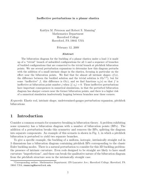
Ineffective perturbations in a planar elastica
Kaitlyn M. Peterson and Robert S. Manning ∗
Mathematics Department
Haverford College
Haverford, PA 19041 USA
February 12, 2009
Abstract
The bifurcation diagram for the buckling of a planar elastica under a load λ is made
up of a “trivial” branch of unbuckled configurations for all λ and a sequence of branches
of buckled configurations that are connected to the trivial branch at pitchfork bifurcation
points. We use several perturbation expansions to determine how this diagram perturbs
with the addition of a small intrinsic shape in the elastica, focusing in particular on the
effect near the bifurcation points. We find that for almost all intrinsic shapes ɛf(s),
the difference between the buckled solution and the trivial solution is O(ɛ 1/3 ), but for
some “ineffective” f, this difference is O(ɛ), and we find functions u j (s) so that f is
ineffective at bifurcation point number j when 〈f, u j 〉 = 0. These ineffective perturbations
have important consequences in numerical simulations, in that the perturbed bifurcation
diagram has sharper corners near the former bifurcation points, and there is a higher risk
of a numerical simulation inadvertently hopping between branches near these corners.
Keywords: Elastic rod, intrinsic shape, undetermined-gauges perturbation expansion, pitchfork
bifurcations
1 Introduction
Consider a common scenario for symmetry-breaking in bifurcation theory. A problem exhibiting
some symmetry has a bifurcation diagram with a number of bifurcation points (BPs). The
addition of a perturbation breaks this symmetry and removes the BPs, splitting the diagram
into separate components. An example of this scenario is shown in Fig. 1, in which a pitchfork
bifurcation is perturbed to yield two separate branches.
To give a specific example, the buckling of a uniform, isotropic, intrinsically straight rod in
3 dimensions has a bifurcation diagram containing pitchfork BPs corresponding to the classic
Euler buckling modes. There is a natural perturbation to consider for this 3D buckling problem:
the presence of intrinsic curvature. Even rods designed to be straight are likely to have small
curvature “imperfections”, and these can break the qualitative nature of the bifurcation diagram
from the pitchfork structure seen in the intrinsically straight case.
∗ Corresponding author: Mathematics Department; 370 Lancaster Ave.; Haverford College; Haverford, PA
19041 USA; rmanning@haverford.edu
1

Figure 1: Standard perturbation of a pitchfork bifurcation into two separate branches
Such elastic rod models have been used to represent the bending and twisting of DNA. For
many DNA sequences, the intrinsic shape is nearly straight, but the minimum-energy stacking
configurations of consecutive base-pairs does introduce small intrinsic bends that depend on
the specific sequence of the DNA. Multiple studies have sought to determine these stacking
configurations as a function of sequence (e.g., [15, 1, 14, 3]), and then derive from these stacking
configurations the corresponding intrinsic curvature for a continuum elastic rod (e.g., [10]).
These DNA models have seen increasing use in studying a phenomenon called “DNA looping”:
the bending and twisting of DNA a few hundreds of basepairs long in response to prescribed
relative positions and orientations of the two ends (these boundary conditions coming
from, for example, a bound protein of known structure [18, 7, 9] or laser tweezer experiments
[16, 11]). Given the wide variety of DNA sequences, and the almost-as-wide variety of parameters
for determining local bending from sequence, it would be beneficial to have an automated
algorithm to compute the lowest-energy components of the bifurcation diagram given specified
choices of DNA sequence, stacking parameters, and boundary conditions. A strong understanding
of the splitting of the unperturbed pitchfork diagram for base cases such as buckling
or periodic boundary conditions is an important precursor to ensuring that such an automated
algorithm finds all relevant components of the diagram.
How typical is the “standard” splitting shown in Fig. 1? We analyzed this question for one
of the simplest bifurcation problems—the buckling of a planar elastica—under the family of
perturbations of (infinitesimal) intrinsic curvature. Like the 3D buckling problem described
above, this problem exhibits a sequence of pitchfork BPs. This 2D problem is useful as a
base case for the more general 3D DNA looping problem. The formulation of 2D bending
is simple enough that closed-form analysis is not too unwieldy; at the same time, it seems
reasonable to suppose that the 3D results would be analogous, since, in some sense, 3D bending
is composed of two orthogonal directions of 2D bending. The particular buckling boundary
conditions we choose yield a classic problem in mechanical engineering, but are not the typical
boundary conditions for DNA looping. Still, a likely computational approach to determining
configurations obeying arbitrary DNA looping boundary conditions would involve beginning
2

from one of a small number of simple configurations, one of which would be the straight-rod
configuration studied here (in addition, to, perhaps, a circle and a semicircle).
Thus, this choice of a simple model problem should allow us to focus on the fundamental
questions of which perturbations are atypical and how the bifurcation diagrams of atypical
perturbations differ from the typical case. Our main finding is that for these atypical cases,
the perturbation of the BP is significantly smaller than in the typical case, leading us to label
these perturbations as “ineffective”.
This question is related to the analysis of “unfolding” a pitchfork bifurcation diagram in
dynamical systems, see, e.g., [5, 8]. The standard example is to consider the algebraic equation
λx − x 3 = 0, which exhibits a pitchfork BP at λ = 0. The addition of a second parameter, e.g.,
α+λx−x 3 = 0, splits the diagram as in Fig. 1 if α ≠ 0. The boundary case α = 0 is the analogue
of the ineffectiveness condition we derive for the elastica, although the analysis and final result
are more involved since our mathematical setting is an ODE (plus boundary conditions and
an integral constraint) rather than an algebraic equation, and the perturbations considered are
a space of functions rather than a single parameter. Furthermore, in the standard unfolding
study, the focus is generally on α = 0 as the transition between qualitative behaviors, whereas
we focus on determining the leading-order behaviors of solutions both away from, and directly
on, this boundary case.
In addition to this theoretical analysis, we present some computational results motivated
by the idea of deriving an automated algorithm to determine DNA looping configurations.
One approach to performing such computations is to use exactly the symmetry-breaking path
considered here: begin with the symmetric problem for which solutions are known, and proceed
via a continuation algorithm to numerical solutions for the perturbed problem. We explore
how these continuation algorithms can fail if the perturbation is ineffective (or even nearly
ineffective), due to the presence of sharp corners in a branch of solutions. Thus, in designing
a system for automatically computing such bifurcation diagrams for a wide range of intrinsic
shapes, the ineffectivity conditions we derive serve as an important red flag that numerical
difficulties may arise in a specific subset of computations.
Our analysis proceeds as follows. First, we formulate the planar buckling problem in Sec. 2,
including an O(ɛ) intrinsic-curvature term. Next, in Sec. 3, we apply a standard perturbation
expansion to the “trivial branch” of ɛ = 0 unbuckled configurations. Away from the BPs, this
expansion gives an O(ɛ) approximation to the perturbation of the trivial branch. At the BPs,
this analysis breaks down for most intrinsic curvature profiles, but for certain special profiles,
it does still yield an O(ɛ) solution. These cases are exactly the ineffective perturbations, and
we derive conditions for when they occur. In Sec. 4, we apply an alternative perturbation
technique called undetermined gauges to the effective perturbations at the BPs and find an
O(ɛ 1/3 ) leading-order term for the perturbation of the unbuckled configuration. Finally, in Sec.
5, we present several examples illustrating the theory and a computational study verifying the
numerical difficulties created by ineffective or nearly ineffective perturbations.
3

2 The planar buckling problem
We consider an inextensible and unshearable elastic rod in the plane, assumed for simplicity to
have total arclength 1. We parametrize the rod by arclength s, and denote the configuration of
the rod at arclength-value s by (x(s), y(s)). We choose coordinates and boundary conditions as
shown in Fig. 2: the s = 0 end of the rod is at the origin, we impose clamped boundary conditions
at each end requiring the tangent vectors to be vertical, and further require x(1) = 0. The
inextensibility-unshearability constraint implies that (x ′ (s), y ′ (s)) is a unit vector; this allows us
to describe the rod by a single unknown function θ(s), where (x ′ (s), y ′ (s)) = (cos θ(s), sin θ(s)).
The clamped boundary conditions are given by θ(0) = θ(1) = 0, and the additional constraint
x(1) = 0 can be rewritten as ∫ 1
sin θ(s)ds = 0.
0
Figure 2: Boundary conditions on the planar elastica. The s = 0 end of the rod is held at the
origin with vertical tangent, while the s = 1 end of the rod is held at x = 0, also with vertical
tangent.
We place a mass m > 0 at the s = 1 end of the rod, and assume the following functional for
the energy of the rod-plus-mass system:
∫ 1
[ K
E[θ] ≡
2 (θ′ (s) − ɛf(s)) 2 + mg cos θ(s)]
ds.
0
The first term represents the bending energy of the rod, and the second term the potential
energy of the load. The term ɛf(s) is used to model intrinsic curvature: the minimum-energy
configuration of the rod has θ ′ (s) = ɛf(s), and deviations from ɛf(s) involve a quadratic energy
cost, weighted by the stiffness parameter K. For simplicity, we express energy in units of K,
and define λ = mg/K > 0, so that the energy functional becomes:
∫ 1
[ 1
E[θ] =
2 (θ′ (s) − ɛf(s)) 2 + λ cos θ(s)]
ds.
0
4

We thus consider the calculus of variations problem to find critical points of E subject to
the boundary conditions θ(0) = θ(1) = 0 and the isoperimetric constraint ∫ 1
sin θ(s)ds = 0.
0
These critical points are found by solving the ordinary differential equation (ODE) defined by
the Euler-Lagrange equation (with Lagrange multiplier µ included because of the isoperimetric
constraint):
θ ′′ (s) = ɛf ′ (s) − λ sin θ(s) + µ cos θ(s).
Thus, the mathematical problem we considered was, given known values for the load λ,
perturbation parameter ɛ, and intrinsic curvature profile f(s) (with f ′ not identically zero,
since otherwise ɛ has no effect), find solutions (θ(s), µ) of
θ ′′ (s) = ɛf ′ (s) − λ sin θ(s) + µ cos θ(s)
θ(0) = θ(1) = 0,
∫ 1
0
sin θ(s)ds = 0.
For ɛ = 0, the solutions to (1) as λ varies yield the familiar force-length diagram seen in
Fig. 3 (all bifurcation diagrams in this article were computed using the parameter-continuation
package AUTO97, http://indy.cs.concordia.ca/auto [4]). One solution (for each value of
λ) is θ(s) ≡ 0, µ = 0 (a straight rod), and this corresponds to the horizontal line at the top of
Fig. 3. We call this the “trivial branch”.
(1)
Figure 3: Bifurcation diagram for a planar elastica with no intrinsic curvature (ɛ = 0). The
height of the top of the rod (y(1)) is plotted against the imposed load λ.
There are pitchfork bifurcation points † at all values of λ satisfying
2 − 2 cos √ λ − √ λ sin √ λ = 0 (2)
† The appearance of the pitchfork bifurcation points in Figure 3 is slightly different than the standard picture
from Figure 1 since the two outer prongs of the pitchfork are folded on top of each other due to the choice of
y(1) as ordinate.
5

(see Sec. 3 for a derivation of this equation). This equation has a countable sequence of solutions
that we will label as 0 < λ 1 < λ 2 < · · · . For n odd, λ n = (n + 1) 2 π 2 , whereas for n even,
(n + 0.5) 2 π 2 < λ n < (n + 1) 2 π 2 with (n + 1) 2 π 2 − λ n → 0 as n → ∞. Two properties of λ n (for
n even) will be useful to us:
Lemma 1. For n even,
sin √ λ n = 4√ λ n
λ n + 4 , cos √ λ n = 4 − λ n
λ n + 4 .
Proof: By (2), we have
1 − cos √ λ n =
Multiplying these two equations, we find:
Collecting terms,
√
λn sin √ λ n
, 1 + cos √ √
λn sin √ λ n
λ n = 2 −
.
2
2
sin √ 2 λ n = √ λ n sin √ λ n − λ n sin √ 2 λ n
.
4
sin √ (
2 λ n 1 + λ )
n
= √ λ n sin √ λ n ,
4
and since sin √ λ n ≠ 0 for n even, we may divide both sides by it and solve for sin √ λ n to find
the desired result.
The formula for cos √ λ n follows from the formula cos √ λ n = − √ 1 − sin √ 2 λ n (note the
minus sign due to the fact that √ λ n is just below an odd multiple of π). □
Lemma 2. For n even, −λ n − λ n cos √ λ n + 2 √ λ n sin √ λ n = 0.
Proof: Since (n + 0.5) 2 π 2 < λ n < (n + 1) 2 π 2 , we have sin √ λ n ≠ 0 and 1 − cos( √ λ n ) ≠ 0.
Thus
sin √ λ n
1 − cos √ λ n
= 1 + cos √ λ n
sin √ λ n
, (3)
since cross-multiplying yields the identity 1 − cos 2 √ λ n = sin 2 √ λ n . By (2), the left-hand side
of (3) equals 2/ √ λ n , and therefore,
1 + cos √ λ n
sin √ λ n
= 2 √
λn
.
Cross-multiplying, and multiplying both sides by √ λ n , yields the desired equality. □
6

3 Perturbation of trivial branch for small ɛ
For fixed λ > 0, f(s), and ɛ > 0, we now seek a solution to (1) that will be close to the solution
on the trivial branch for ɛ = 0. We use a standard perturbation analysis, writing
θ(s) = θ 0 (s) + ɛθ 1 (s) + · · ·
µ = µ 0 + ɛµ 1 + · · ·
The O(1) terms θ 0 (s) and µ 0 vanish since µ = 0 and θ(s) ≡ 0 on the trivial branch. Therefore,
we seek the O(ɛ) terms θ 1 (s) and µ 1 , by plugging these expansions into (1). After Taylor
expanding sin θ and cos θ and isolating the O(ɛ) terms we find:
θ ′′
1 = f ′ (s) − λθ 1 + µ 1 , θ 1 (0) = θ 1 (1) = 0,
∫ 1
0
θ 1 (s)ds = 0. (4)
By a standard integrating factor approach, we find the general solution to the ODE in (4):
θ 1 (s) = √ 1 ∫ s
λ
0
f ′ (t) sin( √ λ(s − t))dt + µ 1
λ + C 1 cos( √ λs) + C 2 sin( √ λs)
When we require that this general solution satisfy the remaining conditions in (4), we find three
linear equations in µ 1 , C 1 , and C 2 :
⎡
⎤ ⎡ ⎤ ⎡
⎤
1/λ 1 0
⎣1/λ cos √ λ sin √ µ 1
0
λ
1/λ (sin √ λ)/ √ λ (1 − cos √ λ)/ √ ⎦ ⎣C 1
⎦ = ⎣ (1/ √ λ) ∫ 1
f ′ (t) sin( √ λ(1 − t))dt
0
λ C 2 (1/ √ λ) ∫ 1 ∫ s
f ′ (t) sin( √ ⎦
λ(s − t))dtds
0 0
(5)
The bottom term on the right-hand side can be simplified by switching the order of integration:
∫ 1 ∫ 1
and then computing the inner integral:
1
λ
0
∫ 1
0
t
f ′ (t)
(√ )
√ sin λ(s − t)
λ
ds dt,
[ (√ )]
f ′ (t) 1 − cos λ(1 − t)
Inserting this into (5), and multiplying both sides by λ, gives:
⎡
⎤ ⎡ ⎤ ⎡
⎤
1 λ 0
⎣1 λ cos √ λ λ sin √ µ 1 √
0
∫
λ
1 √ λ sin √ λ √ λ(1 − cos √ ⎦ ⎣C 1
⎦ = ⎣ 1
λ f ′ (t) sin( √ λ(1 − t))dt
∫ 0
λ) C 1
2 f ′ (t)[1 − cos( √ ⎦ (6)
λ(1 − t))] dt
0
The matrix on the left-hand side has determinant λ 3/2 (2 cos √ λ − 2 + √ λ sin √ λ), so (6) has
a unique solution if 2 cos √ λ − 2 + √ λ sin √ λ ≠ 0. In other words, referring back to (2), we
dt.
7

have shown that away from the bifurcation points, i.e., for λ ≠ λ n , the standard perturbation
expansion yields a solution, i.e., a O(ɛ) approximation to θ(s) near the trivial branch.
(We note that the BP condition (2) can be derived by a computation much like the one just
completed; in that instance, we would be looking for solutions near the trivial branch to the
problem without the f ′ term. We would use the same perturbation expansion, resulting in (6)
but with a zero vector as the right-hand side, and so we would have a nontrivial solution (a
BP) exactly when the determinant of the matrix vanishes.)
What is particularly interesting for our study is whether (6) might have a solution even at
a bifurcation point. Here we can use the following (see, e.g., [17, §3.4]):
Theorem 1. For an n × n matrix A, the column space of A is equal to the orthogonal complement
of the nullspace of A T .
We want to know whether the right-hand side b of (6) is in the column space of the matrix
A on the left-hand side, which by Theorem 1 is true if and only if 〈b, u〉 = 0 for all nullvectors
u of A T . The nullvector for λ = λ n has a different form depending on whether n is odd or
even.
If n is odd, then λ n = (n + 1) 2 π 2 and
⎡
1 1
⎤
1
A T = ⎣(n + 1) 2 π 2 (n + 1) 2 π 2 0⎦ ,
0 0 0
and nullspace (A T ) = span {(−1, 1, 0)}.
If n is even, then there is no obvious simplification to be made to the form of the matrix:
⎡
⎤
1 1 1
A T = ⎣λ
cos √ √ √
λ λ sin λ
0 λ sin √ λ √ λ(1 − cos √ ⎦ ,
λ)
but, using (2) and Lemma 2, it can be verified that nullspace (A T ) = span {(−1, −1, 2)}.
Combining these nullvectors of A T with Theorem 1 shows that (6) has a solution at λ n if
and only if
∫ 1
0
∫ 1
0
f ′ (t) sin( √ λ n (1 − t))dt = 0, for n odd
[ (√ )
f ′ (t) 2 − 2 cos λn (1 − t) − √ (√ )]
λ n sin λn (1 − t) dt = 0, for n even
Intrinsic curvature profiles f satisfying (7) for some n are the “ineffective” perturbations for
bifurcation point λ n .
(7)
4 Undetermined-gauges analysis of bifurcation points
We now turn to the analysis of the bifurcation points λ = λ n . In Sec. 3 we showed that for the
ineffective perturbations defined by (7), the standard perturbation analysis predicts an O(ɛ)
8

lowest-order term for θ 1 and µ 1 , but that this analysis fails for the remaining perturbations. Here
we investigate those cases by applying a more general technique, the methods of undetermined
gauges [12], which is used to derive the leading-order behavior when it does not follow the
standard O(ɛ) pattern.
We are, as before, considering (1), but now we formulate a more general perturbation expansion
for θ and µ. This expansion is computed one term at a time, so we begin by writing:
θ(s) = δ 1 (ɛ)θ 1 (s), µ = δ 1 (ɛ)µ 1 ,
where δ 1 (ɛ) is an unknown function of ɛ that our analysis will determine. We will restrict
attention to the family δ 1 (ɛ) = ɛ a for a real. We insert these expressions into (1) and expand
the sin and cos as Taylor series:
δ 1 θ 1 ′′ = ɛf ′ (s) − λ n (δ 1 θ 1 + · · · ) + (δ 1 µ 1 )(1 + · · · ),
δ 1 θ 1 (0) = δ 1 θ 1 (1) = 0,
∫ 1
0
(δ 1 θ 1 + · · · )ds = 0.
We want to look at the leading order terms, but in the ODE, there is a question of whether δ 1
or ɛ is dominant, or if they could be of the same order. If ɛ were dominant, then the leadingorder
terms of the ODE would be the nonsensical 0 = ɛf ′ (s). If δ 1 and ɛ were of the same
order, i.e., δ 1 = ɛ, then the leading-order terms of the ODE would give the same equation as in
the standard perturbation expansion, which we know from Sec. 3 has no solution. Hence, the
dominant term must be δ 1 , so we keep the O(δ 1 ) terms to find:
θ ′′
1 = −λ n θ 1 + µ 1 , θ 1 (0) = θ 1 (1) = 0,
∫ 1
0
θ 1 (s)ds = 0.
The general solution of the ODE is θ 1 (s) = C 1 cos( √ λ n s) + C 2 sin( √ λ n s) + µ 1 /λ n . Imposing
θ 1 (0) = 0, we find µ 1 = −λ n C 1 , and then the other two conditions give the linear system:
[ √ cos λn − 1 sin √ ] [C1 ] [
λ n 0
sin √ √λn
λ n 1−cos
− 1
√ √λn
λ n
= .
C 2 0]
Since the determinant of the matrix in this system is zero by (2), we have nontrivial solutions
(C 1 , C 2 ), namely any nonzero nullvector of the matrix. If n is odd, the matrix simplifies to
[ ] 0 0
,
−1 0
so that (0, 1) is a nullvector and the solution coming from this first gauge is:
θ 1 = C sin( √ λ n s) = C sin(π(n + 1)s)
µ 1 = 0
(n odd, C ≠ 0 to be determined) (8)
9

On the other hand, if n is even, then (sin √ λ n , 1 − cos √ λ n ) is a nullvector of the matrix, which
means that the solution coming from this first gauge is:
θ 1 = k
[sin √ ( (√ ) )
λ n cos λn s − 1 + (1 − cos √ (√ )]
λ n ) sin λn s
µ 1 = −kλ n sin √ λ n
By (2), 1 − cos √ λ n = 1 2√
λn sin √ λ n , so that this solution can be rewritten as:
θ 1 = k sin √ (√ )
λ n
(cos λn s − 1 + 1 (√ )
λn sin λn s
2√ )
µ 1 = −kλ n sin √ λ n
For simplicity, we write k sin √ λ n /2 as a single constant C for the final form of the solution:
( (√ )
θ 1 = C 2 cos λn s − 2 + √ (√ ))
λ n sin λn s
(n even, C ≠ 0 to be determined) (9)
µ 1 = −2Cλ n
In order to determine C and δ 1 , we add another gauge.
θ = δ 1 (ɛ)θ 1 (s) + δ 2 (ɛ)θ 2 (s), µ = δ 1 (ɛ)µ 1 + δ 2 (ɛ)µ 2 ,
for δ 2 (ɛ) an unknown function of ɛ (again in the family ɛ a ), by definition of lower order in ɛ than
δ 1 . As before, we insert these expressions into (1) and Taylor-expand the sin and cos terms,
looking for the next-lowest-order terms after O(δ 1 ).
For the boundary conditions, these next-lowest-order terms give δ 2 (ɛ)θ 2 (0) = δ 2 (ɛ)θ 2 (1) = 0,
or θ 2 (0) = θ 2 (1) = 0. As for the integral condition, since sin θ = θ − θ 3 /6 + · · · , there are two
next-lowest-order candidates: δ 2 from the θ term, and δ 3 1 from the θ 3 term. We list them both
for the time being:
∫ 1
0
(δ 2 θ 2 (s) − 1 6 (δ 1) 3 θ 1 (s) 3 + · · · )ds = 0, (10)
Finally, we look at the ODE. The sin term yields the same two possible second-lowest-order
terms δ 2 or (δ 1 ) 3 as in the integral condition, and so, in fact, does the cos term (δ 2 from the
δ 2 µ 2 term in µ times the 1 in the cos expansion, or (δ 1 ) 3 from the δ 1 µ 1 term in µ times the
−(δ 1 θ 1 ) 2 /2 from the cos expansion):
δ 2 θ 2 ′′ = ɛf ′ (s) − λ n
[δ 2 θ 2 (s) − 1 ]
6 (δ 1) 3 (θ 1 (s)) 3 + · · ·
+
[
δ 2 µ 2 − 1 ]
2 (δ 1) 3 µ 1 (θ 1 (s)) 2 + · · · . (11)
Overall, there are three candidates for next-lowest-order term: ɛ, δ 2 , and (δ 1 ) 3 . We have to
consider all possibilities for the relative rankings of these terms, including ties. The arguments
below rule out all possibilities except having all three of the same order.
Case 1: ɛ lowest-order
10

This can not be true, since the dominant terms in (11) would give 0 = f ′ (s), but by assumption
f ′ is not identically zero. □
Case 2: (δ 1 ) 3 lowest-order
This can not be true, since the dominant terms in (11) would give 0 = − 1 6 (θ 1(s)) 2 (θ 1 (s)+3µ 1 ),
and neither θ 1 nor θ 1 + 3µ 1 is identically zero. □
Case 3: δ 2 lowest-order
The dominant terms in (11) would give the same equation we solved for θ 1 and µ 1 (including
the boundary and integral conditions), so that θ 2 = θ 1 and µ 2 = µ 1 . Thus, our gauge expansions
would reduce to θ = (δ 1 + δ 2 )θ 1 and µ = (δ 1 + δ 2 )µ 1 , and we would essentially be back where we
began this step, having replaced the unknown δ 1 (ɛ) by another unknown δ 1 (ɛ) + δ 2 (ɛ), without
having learned anything about the connection of δ 1 to ɛ. Thus, we reject this case. □
Case 4: ɛ and (δ 1 ) 3 tied for lowest-order
Since (δ 1 ) 3 = ɛ, the dominant terms in (11) would give 0 = f ′ (s) − 1 6 (θ 1(s)) 3 . This requires
the perturbation f ′ to take the very particular form of the cubes of the functions (8) or (9).
Since this case does not yield a solution for a general perturbation, we reject this case. □
Case 5: ɛ and δ 2 tied for lowest-order
This can not be true: we would have δ 2 = ɛ and the dominant terms in (11) would give the
same equation (4) from the standard perturbation expansion, as well as the same integral and
boundary conditions, and we know that this system has no solution for λ = λ n and the effective
perturbations we are considering in this section. □
Case 6: δ 2 and (δ 1 ) 3 tied for lowest order
We have (δ 1 ) 3 = δ 2 and the dominant terms in (11) would give
θ ′′
2 = −λ n θ 2 + 1 6 λ n(θ 1 ) 3 + µ 2 − 1 2 µ 1(θ 1 ) 2 .
This equation can be solved in closed form using the forms of µ 1 and θ 1 from (8) and (9).
For example, for n odd, we have µ 1 = 0 and θ 1 = C sin( √ λ n s), and the ODE has solution:
θ 2 (s) = C 1 cos( √ λ n s) + C 2 sin( √ λ n s) + µ 2
− C3 s √ λ n cos( √ λ n s)
λ n 16
Applying θ 2 (0) = θ 2 (1) = 0 leads to the impossible conclusion that C = 0.
For n even, the ODE solution is:
+ C3 sin(3 √ λ n s)
.
192
θ 2 (s) = C 1 cos( √ λ n s) + C 2 sin( √ λ n s) + µ 2
+ 8C3
λ n 3 + C3
16 (λ n − 12)(2 − λ n s) cos( √ λ n s)
+ C3
96 (3λ n − 4) cos(3 √ λ n s) + C3
192
√
λn (λ n − 12)[24s sin( √ λ n s) + sin(3 √ λ n s)]
11

The condition θ 2 (0) = 0 allows us to solve for µ 2 , leaving:
θ 2 (s) = C 1 [cos( √ λ n s) − 1] + C 2 sin( √ λ n s) + C3 (148 − 15λ n )
96
+ C3
16 (λ n − 12)(2 − λ n s) cos( √ λ n s) + C3
96 (3λ n − 4) cos(3 √ λ n s)
+ C3 √
λn (λ n − 12)[24s sin( √ λ n s) + sin(3 √ λ n s)]
192
Next we impose the boundary condition θ 2 (1) = 0, and using Lemma 1, we find:
(12)
θ 2 (1) = − 2λ n
C 1 + 4√ λ n
C 2 + C3 λ 2 n(λ n − 12)
4 + λ n 4 + λ n 16(4 + λ n )
Recalling (10), since δ 2 = (δ 1 ) 3 , the integral condition is:
∫ 1
[θ 2 (s) − 1 ]
6 (θ 1(s)) 3 ds = 0.
Again using Lemma 1, we can simplify this to:
0
= 0. (13)
−
λ n
C 1 + 2√ λ n
C 2 + C3 λ n (20 + λ n )
4 + λ n 4 + λ n 8(4 + λ n )
= 0. (14)
Subtracting two times (14) from (13) gives:
C 3 λ 2 n(λ n − 12)
16(4 + λ n )
− C3 λ n (20 + λ n )
4(4 + λ n )
= C3 λ n (λ n − 20)
16
which implies either C = 0, λ n = 0, or λ n = 20, none of which is true. □
Having ruled out all other cases, we can conclude that δ 2 , (δ 1 ) 3 and ɛ are all of the same
order, i.e., δ 1 = ɛ 1/3 and δ 2 = ɛ. In particular, we have shown that θ = O(ɛ 1/3 ).
In fact, this second gauge allows us to completely determine the leading-order behavior of
θ(s) and µ, as summarized by the following theorem:
Theorem 2. For n odd,
with
θ(s) = Cɛ 1/3 sin( √ λ n s) + · · ·
µ = ɛµ 2 + · · ·
λ n = π(n + 1)
( ∫ 16 1
C = f ′ (t) sin( √ ) 1/3
λ n (1 − t))dt
λ n 0
∫ 1 [
µ 2 = − f ′ (t) 1 − cos( √ ]
λ n (1 − t)) dt,
0
12
= 0,

For n even,
(√ )
θ(s) = Cɛ
(2 1/3 cos λn s − 2 + √ (√ ))
λ n sin λn s + · · ·
µ = −2ɛ 1/3 Cλ n + · · ·
with
(
16
C =
(λ n ) 2 (λ n − 20)
∫ 1
0
[
f ′ (t) 2 − 2 cos( √ λ n (1 − t)) − √ λ n sin( √ ] 1/3
λ n (1 − t)) dt)
.
Proof: For n even, all that remains is to determine C, while for n odd, we must compute C
and µ 2 . The derivation largely follows the computations in Case 6. The ODE to be solved is:
θ ′′
2 = f ′ − λ n θ 2 + 1 6 λ n(θ 1 ) 3 + µ 2 − 1 2 µ 1(θ 1 ) 2 , (15)
identical to Case 6 except for the addition of f ′ to the right-hand side. Therefore, the ODE
solution will be the expression found in Case 6 plus the term
∫
1 s
√ f ′ (t) sin( √ λ n (s − t))dt, (16)
λn
0
the solution to the equation θ ′′
2 = f ′ − λ n θ 2 seen in Sec. 3. Since this new term vanishes at
s = 0, it will have no effect on the first step from Case 6: eliminating µ 2 using θ 2 (0) = 0.
Thus, for n odd, the solution to (15) plus θ 2 (0) = 0 is
θ 2 (s) = C 1 [cos( √ λ n s) − 1] + C 2 sin( √ λ n s) − C3 s √ λ n cos( √ λ n s)
16
+ C3 sin(3 √ λ n s)
+ 1 ∫ s
√ f ′ (t) sin( √ λ n (s − t))dt.
192 λn
Next we impose the condition θ 2 (1) = 0 to find the given formula for C. Note that the integral
does not vanish (and hence C ≠ 0 as required) since that is our definition of what makes a
perturbation f ′ effective.
Finally, we impose the condition ∫ 1
θ 0 2(s)ds = 0 (for n odd, (θ 1 ) 3 = sin 3 (π(n + 1)s) has zero
integral so this term drops out of the integral condition) to find:
C 1 = √ 1 ∫ 1
λn
0
∫ s
0
f ′ (t) sin( √ λ n (s − t)) dt ds = 1 λ n
∫ 1
0
0
[ (√ )]
f ′ (t) 1 − cos λn (1 − t)
(the second equality comes from switching the order of integration as in Sec. 3). Since µ 2 =
−C 1 λ n (from the θ 2 (0) condition), we find the given formula for µ 2 .
dt
13

For n even, the solution to (15) plus θ 2 (0) = 0 is (12) plus the term (16). Using the same
steps as in Case 6, the boundary condition θ 2 (1) = 0 and the integral condition yield the
equations:
− 2λ n
C 1 + 4√ λ n
C 2 + C3 λ 2 n(λ n − 12)
+ 1 ∫ 1
√ f ′ (t) sin( √ λ n (1 − t))dt = 0
4 + λ n 4 + λ n 16(4 + λ n ) λn 0
−
λ n
C 1 + 2√ λ n
C 2 + C3 λ n (20 + λ n )
+ 1 ∫ 1
f ′ (t)(1 − cos( √ λ n (1 − t)))dt = 0.
4 + λ n 4 + λ n 8(4 + λ n ) λ n
Subtracting twice the second equation from the first yields the given formula for C. □
0
5 Examples
5.1 Bifurcation diagrams with effective and ineffective perturbations
We consider four perturbation f ′ : f ′ 1 that is effective for BPs # 1 and 2, f ′ 2 that is ineffective
for BP # 1 and effective for BP # 2, f ′ 3 that is effective for BP # 1 and ineffective for BP #
2, and f ′ 4 that is ineffective for BPs # 1 and 2. Specifically, we first define:
u 1 (s) = √ 2 sin( √ λ 1 (1 − s)),
1
u 2 (s) = √
[2 − 2 cos( √ λ 2 (1 − s)) − √ λ 2 sin( √ ]
λ 2 (1 − s)) ,
λ2
i.e., length-1 elements in L 2 in the directions of the functions that define ineffectiveness for BPs
# 1 and 2, in the sense that f ′ is ineffective at BP # n if 〈f ′ , u n 〉 = 0. We note that u 1 and u 2
are orthogonal.
We define our four perturbations as follows: f ′ 1 = (u 1 +u 2 )/ √ 2, f ′ 2 = u 2 , f ′ 3 = u 1 , and f ′ 4(s) =
√
2π2 − 3(s + sin(2πs)/π)/(π √ 6). By design, all f ′ j are length-1 (to allow fair comparisons
among them); f ′ 2 is orthogonal to u 1 , f ′ 3 is orthogonal to u 2 , f ′ 4 is orthogonal to both u 1 and
u 2 ; and all other pairings of f ′ j with u k are not close to orthogonal.
The bifurcation diagrams for these perturbations, with ɛ = 1, are shown in Fig. 4. The difference
between effective and ineffective perturbations is clear: in each case where a perturbation
is effective, the diagram is relatively smooth near the former BP, whereas in the ineffective
cases, the diagram has a sharp corner. Indeed, to numerically compute some of these corners
required a significant amount of care, e.g., the use of a very small stepsize, or a temporary
increase in ɛ by an order of magnitude just to get onto the perturbation of the bifurcating
branch.
5.2 Leading-order behaviors in ɛ
Finally, we show two examples illustrating the lowest-order expressions for θ(s) and µ found
in Sec. 4. In our first example, We take f ′ (s) = s, a perturbation that is effective at λ = λ 1
14

Figure 4: Bifurcation diagrams for elastica perturbed by intrinsic curvature profiles f ′ (see text
for specific functions used). (a) effective perturbation at BP # 1 and 2; (b) ineffective at BP
# 1, effective at BP # 2; (c) effective at BP # 1, ineffective at BP # 2; (d) ineffective at BP
# 1 and 2.
15

Figure 5: Graphs of θ(s) for f ′ (s) = s, λ = λ 1 , λ 2 and ɛ = 1/4, 1/2, and 1. For λ = λ 1 , the
dependence of θ on ɛ appears to be larger than O(ɛ), in line with the O(ɛ 1/3 ) prediction of the
theory. The values of θ(1/4) (the maxima) and µ are reported in the inset table. For λ = λ 2 ,
the dependence of θ on ɛ appears to be approximately O(ɛ), in line with the fact that f ′ is
ineffective at λ 2 .
(〈f ′ , u 1 〉 = 0.39) and ineffective at λ = λ 2 (〈f ′ , u 2 〉 = 0). In Fig. 5, we show the graphs of θ(s)
for λ = λ 1 , λ 2 , and for ɛ = 1/4, 1/2, and 1.
Our theoretical prediction for the behavior at λ = λ 1 comes from Theorem 2 (since f ′ is
effective). We compute λ 1 = 2π,
and
( ∫ 16 1
1/3
C = t sin(2π(1 − t))dt)
= 0.401,
4π 2
µ 2 = −
∫ 1
0
0
t(1 − cos(2π(1 − t)))dt = −0.5.
Thus, our predicted behavior at λ = λ 1 is θ(s) ≈ 0.401ɛ 1/3 sin(2πs), µ ≈ −0.5ɛ. The shape
of the actual solution θ(s) in Fig. 5 matches the predicted sin(2πs), and the scaling with ɛ
is clearly larger than O(ɛ). Furthermore, from the table inset in the figure, we see that both
θ(1/4) (the heights of the peaks) and µ are close matches with our predicted formulas.
As for λ = λ 2 , since f ′ satisfies the ineffectivity condition, we expect θ(s) to have O(ɛ)
behavior rather than O(ɛ 1/3 ). Indeed, we see in Fig. 5 that this appears to be the case, as
θ(s) appears to be roughly halved when ɛ is halved. In this case, our theory does not give a
predictive formula for the leading-order behavior of θ(s) or µ; the system (6) has an infinite
number of solutions, and one would have to proceed to higher-order terms in the standard
perturbation expansion in order to determine which of these solutions is relevant.
In our second example, we take f ′ (s) = sin(3πs), a perturbation that is ineffective at λ = λ 1
(〈f ′ , u 1 〉 = 0) and is effective at λ = λ 2 (〈f ′ , u 2 〉 = −0.67). In Fig. 6, we show the graphs of
θ(s) for λ = λ 1 , λ 2 and ɛ = 1/4, 1/2, and 1.
16

Figure 6: Graphs of θ(s) for f ′ (s) = sin(3πs), λ = λ 1 , λ 2 and ɛ = 1/4, 1/2, and 1. For λ = λ 1 ,
the dependence of θ on ɛ appears to be approximately O(ɛ), in line with the fact that f ′ is
ineffective at λ 1 . For λ = λ 2 , the dependence of θ on ɛ appears to be larger than O(ɛ), in line
with the O(ɛ 1/3 ) prediction of the theory. The values of θ(1/2) and µ are reported in the inset
table.
Our theoretical prediction for the behavior at λ = λ 2 comes from Theorem 2 (since f ′ is effective).
Using the formulas in that theorem, we compute λ 2 = 80.7629 and C = 0.05557. Thus,
our predicted behavior at λ = λ 2 is θ(s) ≈ −0.05557ɛ 1/3 (2 cos(8.987s) − 2 + 8.987 sin(8.987s)),
µ ≈ 8.976ɛ 1/3 . The shape of the actual solution θ(s) in Fig. 6 matches the predicted functional
form, and the scaling with ɛ is clearly larger than O(ɛ). Furthermore, from the table inset in
the figure, we see that both θ(1/2) (which from our theoretical formula should equal 0.623ɛ 1/3 )
and µ are close matches with our predicted formulas.
5.3 Computational Impact
Apart from an interest in understanding on a theoretical level how a shape perturbation affects
the bifurcation diagram for buckling, we were also motivated by a pragmatic concern: to what
extent ineffective perturbations would interfere with the design of an automated algorithm to
compute bifurcation diagrams for a given intrinsic shape. The sharp corners in Fig. 4bcd suggest
potential computational challenges, and we explored that question more concretely with the
following numerical study.
We generated intrinsic shapes in three different categories (“random”, “nearly ineffective”,
and “ineffective”) as follows. Let f 1 (s), f 2 (s), f 3 (s), f 4 (s) be the Gram-Schmidt orthonormal
basis (in L 2 ([0, 1])) generated by the functions {s, s 2 , s 3 , s 4 }: f 1 (s) = √ 3s, f 2 (s) = 4 √ 5s 2 −
3 √ 5s, f 3 (s) = 15 √ 7s 3 − 20 √ 7s 2 + 6 √ 7s, f 4 (s) = 168s 4 − 315s 3 + 180s 2 − 30s. The intrinsic
shape function f ′ (s) is defined as a linear combination of these basis functions c 1 f 1 (s)+c 2 f 2 (s)+
c 3 f 3 (s) + c 4 f 4 (s), where the coefficients c i are chosen according to different rules for the three
cases. For a “random” perturbation, we choose four independent random numbers x 1 , x 2 ,
17

x 3 , x 4 from a normal distribution with mean 0 and standard deviation 1, and then define
c j = x j / √ (x 1 ) 2 + (x 2 ) 2 + (x 3 ) 2 + (x 4 ) 2 . For an “ineffective” perturbation, we choose x 1 , x 2 ,
x 3 as above, but then set x 4 such that f ′ (s) is ineffective (according to the n = 1 case of Eq.
(7)), and then normalize to define the c j as in the “random” case. For a “nearly ineffective”
perturbation, we generate x 1 , x 2 , x 3 , x 4 as in the ineffective case, but then add to x 4 a random
number with normal distribution with mean 0 and standard deviation 0.01, before normalizing
to define the c j as in the “random” case.
Given each intrinsic shape, we performed a parameter continuation computation in AUTO97
to attempt to compute the first branch of buckled configurations for that intrinsic shape. We
began the computation with λ = 28, zero intrinsic shape, and a straight rod configuration.
Then we turned on the intrinsic shape via parameter continuation, by multiplying the intrinsic
shape function f ′ (s) by a parameter µ that was slowly increased from 0 (no intrinsic shape) to
1 (intrinsic shape determined by f ′ ). Then we increased λ to a target maximum value of 50. A
successful computation would follow the bend of the branch of solutions, with significant rod
buckling occurring around λ = 4π 2 and continuing until λ reaches 50 (cf. Fig. 4a). However, in
cases where a sharp corner exists near λ = 4π 2 (as in Fig. 4bd), the computation could jump
branches and end at a nearly straight configuration at λ = 50.
To assess in an automated way the success of this computation, we did a third parameter
continuation step that decreased µ from 1 back down to 0. Thus, successful runs end at the
λ = 50 point on the first bifurcating branch for the intrinsically-straight rod (i.e., Fig. 3), while
unsuccessful runs end with the rod completely extended. Inspection of the value of y(1) at the
end of the third parameter continuation step allowed easy distinction of these two cases.
Results of these computations are shown in Table 1. The body of the table shows the
percentage of successful runs out of a total of 300 attempts. To give a sense of variability of these
results, we report in parentheses the corresponding standard deviation for a binomial random
variable with N = 300 and p taken as the observed percentage of successes: σ = √ p(1 − p)/N.
(For results reported as 100% (or 0%), all (or none) of the 300 computations were successful,
and thus no meaningful estimate of σ can be provided).
AUTO97 allows a variety of parameter-stepping algorithms, and Table 1 shows the results
for six different approaches: three with fixed step-size and three with variable step-size. The
step-sizes ∆τ are in terms of a “pseudo-arclength” that is a combination of the change in the
parameter value λ and the change in the solution vector of the discretized Euler-Lagrange
equations (1); this approach allows the traversing of “folds” in the bifurcation diagram where
∆λ = 0. Thus, one can informally think of the change in the parameter λ in each step as
being some fraction of ∆τ (though what that fraction is will vary according to the change in
the solution vector at that point on the branch). For the variable step-size computations, the
step-size ∆τ is allowed to varying over two orders of magnitude, with an initial value in the
middle (e.g., (∆τ) init = 0.02 with 0.002 ≤ ∆τ ≤ 0.2 throughout the computation in row 4 of
Table 1). AUTO97 adjusts the step-size with each step according to the convergence properties
of the previous step, striving to take smaller steps when the convergence is more difficult.
Random and ineffective shapes behave radically differently for the range of step-sizes shown
here, and even the nearly ineffective shapes show a relatively high rate of computational failure,
suggesting that this phenomenon will be met in practice for some shapes (despite the fact that
18

Continuation Random Nearly Ineffective Ineffective
Method Shape Shape Shape
∆τ = 0.02 100% 41% (±3%) 0%
∆τ = 0.04 100% 16% (±2%) 0%
∆τ = 0.1 100% 0.7% (±0.5%) 0%
0.002 ≤ ∆τ ≤ 0.2 99.7% (±0.3%) 7% (±2%) 5% (±1%)
0.004 ≤ ∆τ ≤ 0.4 99.7% (±0.3%) 21% (±2%) 5% (±1%)
0.01 ≤ ∆τ ≤ 1 98.7% (±0.7%) 3% (±0.9%) 0%
Table 1: Percentage of successful computations of the first branch of buckled configurations
for different intrinsic shapes: those that are ineffective (according to the theory sketched in
Sec. 3), those that are nearly ineffective (small perturbations of exactly ineffective shapes),
and randomly chosen shapes (see text for detailed descriptions of the three cases). Each row
represents a different step-size strategy within the AUTO97 parameter continuation algorithm.
the set of precisely ineffective shapes is measure zero). As would be expected, for fixed stepsizes,
smaller step-sizes are more successful, though of course at the cost of computation time.
(Even for ineffective perturbations, a sufficiently small step-size will yield successful branch
tracking, though ∆τ needs to be significantly smaller than 0.02). For variable step-sizes, the
data suggests a more complicated situation, including some behavior in the nearly ineffective
column that is not monotonic with step-size bounds. This might be explained by the fact
that the automated step-size adjustment presumably increases the step-size consistently in the
early part of the computation when the rod is barely changing, and this increased step-size
might increase the probability of jumping over a corner in the branch (though the likelihood of
this jump might also depend sensitively on the initial point chosen, since that could determine
whether the jump happens to straddle the corner). Further study would be needed to fully
understand this behavior, but it seems clear at least that the ineffectivity condition derived
here is a useful flag for intrinsic shapes that call for a strong decrease in the step-size used.
Acknowledgments: This work was supported by NSF grant DMS-0384739.
19

References
[1] A. Bolshoy, P. McNamara, R. E. Harrington, and E. N. Trifonov. Curved DNA without
A-A: Experimental estimation of all 16 wedge angles. Proc. Natl. Acad. Sci. USA, 88:2312–
2316, 1991.
[2] L. Czapla, D. Swigon, and W. Olson. Sequence-dependent effects in the cyclization of
short dna. J. Chem. Theory Comput., 2:685–695, 2006.
[3] S.B. Dixit, D.L. Beveridge, D.A. Case, T.E.˜Cheatham III, E. Giudice, F. Lankas, R.
Lavery, J.H. Maddocks, R. Osman, H. Sklenar, K.M. Thayer, and P. Varnai. Molecular
dynamics simulations of the 136 unique tetranucleotide sequences of DNA oligonucleotides.
II. sequence context effects on the dynamical structures of the 10 unique dinucleotide steps.
Biophys. J., 89:3721–3740, 2005.
[4] E. J. Doedel, H. B. Keller, and J. P. Kernévez. Numerical analysis and control of bifurcation
problems, parts I and II. Int. J. of Bif. and Chaos, 3, 4:493–520, 745–772, 1991.
[5] P. Glendinning. Stability, instability and chaos: An introduction to the theory of nonlinear
differential equations. Cambridge Texts in Applied Mathematics. Cambridge University
Press, Cambridge, 1994.
[6] A. Goriely and M. Tabor. Spontaneous helix hand reversal and tendril perversion in
climbing plants. Phys. Rev. Lett., 80:1564–1567, 1998.
[7] S. Goyal, T. Lillian, S. Blumberg, J.-C. Meiners, E. Meyh ofer, and N.C. Perkins. Intrinsic
curvature of DNA influences LacR-mediated looping. Biophys. J., 93:43424359, 2007.
[8] G. Iooss and D.D. Joseph. Elementary Stability and Bifurcation Theory. Undergraduate
Texts in Mathematics. Springer-Verlag, New York, 1980.
[9] J.D. Kahn and D.M. Crothers. Measurement of the DNA bend angle induced by the
Catabolite Activator Protein using Monte Carlo simulation of cyclization kinetics. J. Mol.
Biol., 276:287–309, 1998.
[10] R. S. Manning, J. H. Maddocks, and J. D. Kahn. A continuum rod model of sequencedependent
DNA structure. J. Chem. Phys., 105:5626–5646, 1996.
[11] J. Marko and E.D. Siggia. Stretching DNA. Macromolecules, 28:8759–8770, 95.
[12] J.A. Murdock. Perturbations: Theory and Methods. Classics in Applied Mathematics.
SIAM, Philadelphia, 1999.
[13] W. K. Olson. Simulating DNA at low resolution. Current Opinion in Structural Biology,
6:242–256, 1996.
[14] W.K. Olson, A.A. Gorin, X.J. Lu, L.M. Hock, and V.B. Zhurkin. DNA sequence-dependent
deformability deduced from protein-DNA crystal complexes. PNAS, 95:11163–11168, 1998.
20

[15] P. De Santis, A. Palleschi, M. Savino, and A. Scipioni. Theoretical prediction of the
gel electrophoretic retardation changers due to point mutations in a tract of Sv40 DNA.
Biophys. Chem., 42:147–152, 1992.
[16] Y. Seol, J. Li, P.C. Nelson, T.T. Perkins, and M.D. Betterton. Elasticity of short
DNA molecules: Theory and experiment for contour lengths of 0.6–7 µm. Biophys. J.,
93:43604359, 2007.
[17] T. Shifrin and M.R. Adams. Linear Algebra: a geometric approach. W.H. Freeman, New
York, 2002.
[18] D. Swigon, B.D. Coleman, and W.K. Olson. Modeling the Lac repressor-operator assembly.
I. the influence of DNA looping on Lac repressor conformation. PNAS, 103:9879–9884,
2006.
[19] Y. Zhang and D.M. Crothers. Statistical mechanics of sequence-dependent circular dna
and its application for dna cyclization. Biophysical Journal, 84:136–153, 2003.
21