Second Law analysis of periodic heat conduction through a wall

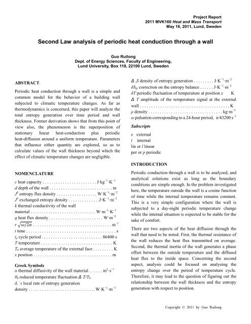
Project Report
2011 MVK160 Heat and Mass Transport
May 16, 2011, Lund, Sweden
Second Law analysis of periodic heat conduction through a wall
Guo Ruilong
Dept. of Energy Sciences, Faculty of Engineering,
Lund University, Box 118, 22100 Lund, Sweden
ABSTRACT.
Periodic heat conduction through a wall is a simple and
common model for the behavior of a building wall
subjected to climatic temperature changes. As far as
thermodynamics is concerned, this paper will analyze the
total entropy generation over time period and wall
thickness. Former derivation shows that from this point of
view also, the phenomenon is the superposition of
stationary linear heat-conduction plus periodic
heat-diffusion around a uniform temperature. Parameters
that influence either quantity are explored, so as to
calculate values of the wall thickness beyond which the
effect of climatic temperature changes are negligible.
NOMENCLATURE
−1
c heat capacity . . . . . . . . . . . . . . . . . . . . . . . . J·kg
−1·K
d depth of the wall . . . . . . . . . . . . . . . . . . . . . . . . . . . . m
J S −2
entropy flux density . . . . . . . . . . . . . . . . . . W·K
−1·m
J S −2
exchanged entropy density . . . . . . . . . . . . . .J·K
−1·m
k thermal conductivity of the wall
−1
material . . . . . . . . . . . . . . . . . . . . . . . . . . . . . W·m
−1·K
q heat flux density . . . . . . . . . . . . . . . . . . . . . . . . W·m −2
r . . . . . . . . . . . . . . . . . . . . . . . . . . . . . . . . . . . m −1
t time . . . . . . . . . . . . . . . . . . . . . . . . . . . . . . . . . . . . . . . . s
t p cycle period . . . . . . . . . . . . . . . . . . . . . . . . . . . 86400 s
T temperature . . . . . . . . . . . . . . . . . . . . . . . . . . . . . . . . K
T 0 average temperature of the external face . . . . . . . . . K
x position . . . . . . . . . . . . . . . . . . . . . . . . . . . . . . . . . . . m
Δ
Greek Symbols
−1
α thermal diffusivity of the wall material . . . . . . m
2·s
θ 0 reduced temperature fluctuation Δ T/T 0
δ i ˙s local rate of entropy generation
−3
density . . . . . . . . . . . . . . . . . . . . . . . . . . . . .. W·K
−1·m
−2
i S density of entropy generation . . . . . . . . . J·K
−1·m
−2
δS lp correction on the entropy balance . . . . . . J·K
−1·m
δT periodic fluctuation of temperature at position x K
Δ T amplitude of the temperature signal at the external
wall . . . . . . . . . . . . . . . . . . . . . . . . . . . . . . . . . . . . . . . . K
ρ density . . . . . . . . . . . . . . . . . . . . . . . . . . . . . . . . . kg·m −3
ω pulsation corresponding to a 24-hour period, π/43200 s −1
Subscripts
e external
i internal
lin or l linear
per or p periodic
INTRODUCTION
Periodic conduction through a wall is to be analyzed, and
analytical solutions exist as long as the boundary
conditions are simple enough. In the problem investigated
here, the temperature outside the wall is a cosine function
of time while the internal temperature remains constant.
This is a very simple configuration where the wall is
subjected to a day-night periodic temperature change
while the internal situation is expected to be stable for the
sake of comfort.
There are two aspects of the heat diffusion through the
wall that need to be noted. First, the thermal resistance of
the wall reduces the heat flux transmitted on average.
Second, the thermal inertia of the wall generates a phase
offset between the outside temperature and the diffused
heat flux to the inside space. Concerning the second
aspect, analysis could be focused on analyzing the
entropy change over the period of temperature cycle.
Therefore, it may lead to the question of figuring out the
relationship between the wall thickness and the entropy
generation with respect to position.
Copyright © 2011 by Guo Ruilong

Ideal processes, second-law analysis are used to evaluate
the problem. Heat diffusion is the only source of
irreversibility, and the calculation of total entropy change
is the main part of this paper. The sensitivity of the results
with respect to heat capacity or climatic conditions is
studied.
PROBLEM STATEMENT
The model used to investigate this problem is that a solid
wall, single-phase, homogeneous, is subjected to a
fluctuating external temperature and an ideally constant
internal temperature. The boundary conditions are:
(1)
and to the boundary conditions, it is easily shown that the
solution for temperature is the sum of a linear component
between T 0 and T i (denoted linear in the following) plus a
purely sinusoidal component (denoted periodic in the
following):
, with
and
with
and
(2)
(3)
where r
stands for . From those equations, it can easily be
seen that the heat flux density q (given by the Fourier’s
law:
) is the sum of two components, a
constant and uniform one derived from the gradient of
, plus a purely periodic one derived from the gradient
of . The total heat flux density is thus:
(4)
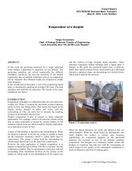
Figure 1. Schematic representation of the studied case
As is shown in Figure 1, the amplitude for external
temperature change is , which is arbitrarily fixed at 15
K. The inner temperature Ti is fixed at 25 ◦C. We also
consider three values of T 0 : , called ―standard case‖
in the following and more or less representing conditions
in summer; , with equality between T 0 and , as it
often occurs in spring or autumn; and , that we
schematically denote as winter. The standard material of
the wall is defined by:
and
Only the periodic regime is considered. After the period
, the wall recovers the same thermodynamical state, and
the change of any state function (e.g., temperature,
internal energy and entropy) is zero over a period.
According to the partial derivative equation ( )
At this point of the development, let us refer to the
well-known problem of the 1D semi-infinite wall
submitted to a cosine temperature change on its boundary
. With our notations, the periodical solution for
temperature is:
Inside the semi-infinite wall, the amplitude of the
temperature signal decreases as i.e. the amplitude
is 10% of the external constraint for
for our standard case), and only 5% for
. It can reasonably be said that the
external temperature signal is almost completely filtered
beyond the position .
In the present problem, the wall depth is finite and
temperature is fixed at the internal boundary; moreover
we are mainly interested in heat fluxes. If one compares
the amplitudes of the (periodical) heat flux density, first
at the internal boundary of the finite wall with depth d,
and second at the position in the semi-infinite wall,
Copyright © 2011 by Guo Ruilong

then, for , the former amplitude is about twice
the latter (exactly twice for thick walls). Indeed, fixing
temperature at a given position is a constraint that
increases the heat flux compared to the semi-infinite wall.
As a result, the internal boundary of a finite wall with d =
0.5 m is as active as the position x = 0.38 m in the
semi-infinite wall, so that considering walls as thick as
0.5 m is relevant in the present problem.
LITERATURE SURVEY
F. Strub, M. Strub, J. Castaing-Lasvignottes, J.P.
Bédécarrats, [3] has done a research on this specific topic
and they has also analyzed it using another method: the
Carnot cycle to calculating the optimal energy
consumption to keep the internal temperature constant.
This approach generates a different results from the one
used in this paper, which raises questions and further
study.
PROJECT DESCRIPTION
-----Analysis based on entropy generation
The local rate of entropy generation density in
one-dimensional heat diffusion is well known:
Once T and q are known, integration of over space
and time yields the total entropy generation over the cycle.
However, in the periodic regime, the analysis is easier to
develop when considering the rates of entropy flux
densities
at the boundaries, the balance of
which, integrated over the cycle period tp, is the total
entropy generation :
At the internal boundary, , the temperature is fixed
at . Developing the heat flux according to Eq. (4), and
considering that the integral of the periodic part over the
cycle period vanishes ( ), it appears that the total
entropy flux density at the internal boundary only
involves the stationary heat flux:
(5)
(6)
At the external face (x = 0), the boundary condition (1)
can be written slightly differently:
The
entropy flux involves Denoting ,
which surely is less than 1 (in our case ), the
expansion in series of is:
In the following, this expansion
will be limited to the first terms and the notation is
used only in series expansions. As for heat flux, the linear
and periodic parts of the entropy flux, and in
rates, are considered. The former is obviously
. Developing as described above
up to , and remembering that only the even powers
of have non-zero integrals over the cycle period,
leads to the entropy flux over a cycle
The periodic part of
heat flux density at
involves the periodic part of the
given by:
The time dependence involves terms in and terms
in . Combination with the expansion of
yields terms in or in .
Here again, only the even powers of have
non-zero integrals over the cycle period. Additional
algebra yields the time integral of :
The entropy fluxes can be rearranged differently,
evidencing an interesting property of the total entropy
generation. Indeed, Eq. (5) can be rewritten as:
or
(7)
, a form which introduces the two
following quantities and
Simple developments with the first terms of
the above-described expansions lead to:
Copyright © 2011 by Guo Ruilong

And
This development demonstrates that the total entropy
generation can be represented as the sum of three
quantities. The first, , is the entropy generation of
stationary heat conduction along the average linear
temperature gradient; is completely independent of
_T . The second, , is the entropy generation of purely
periodic heat diffusion in the wall oscillating around the
temperature T0 with Eq. (1) as constraint; is
(8)
(9)
completely independent of Ti . The third quantity, ,
is only a correction (on the order of when compared
to with a sign opposite to that of ( ).
in the present case), beyond which
hardly
changes. As a consequence the curve presents a
knee at that same abscissa. According to these results, it
could be deduced that the only effect of increasing the
wall thickness beyond that minimum consists in reducing
heat conduction thanks to a larger thermal resistance,
without any effect related to the periodic heat conduction.
CONCLUSIONS
Periodic heat conduction through a wall is a practical
problem, and the case studied above is simplified by
regarding the wall as homogeneous, the internal
temperature as constant and the day-night cycle as
unchanged all year. The analysis of this problem leads to a
better understanding of the heat conduction through the
wall, which consists of two parts: stationary heat diffusion
and periodic one. Second law and entropy generation are
used as the approach to tackle the problem herein, and the
results, to certain degree, shows an evidencing value of
the wall thickness, beyond which entropy generation
hardly changes. However, given the assumptions, this
result can be different to the ones get through other
methods. Therefore, further research concerning this
problem should be done with other approaches and more
realistic circumstances, so as to gain better understanding
of the real problem.
Figure 2. Entropy generation as a function of wall depth. Linear
component , periodic component , total , and sum
.
Fig. 2 presents the curves , and as
functions of the wall depth d for the standard case.
Several features are noteworthy. First, the curve
is a very good approximation of : the
total entropy generation is practically the sum of
stationary heat conduction through the wall between
and , plus periodic heat diffusion in the wall averagely
at T0. Second, and are very similar for thin
walls ( ), but for thick walls ( ) the
former tends to vanish while the latter tends toward an
asymptotic value. Third, the periodic entropy generation
exhibits a minimum at a position (
REFERENCES
[1] A. Bejan, Entropy Generation Minimization,
CRC Press, Boca Raton, NY,ISBN 0-8493-96514,
1996.
[2] E. Johannessen, L. Nummedal, S. Kjelstrup,
Minimizing the entropy generation in heat
exchange, Int. J. Heat Mass Transfer 45 (13)
(2002) 2649–2654.
[3] F. Strub, M. Strub, J. Castaing-Lasvignottes, J.P.
Bédécarrats, Incidence de la nature d’une paroi
sur la production d’entropie en régime thermique
variable, in: Actes du Colloque Franco-Roumain
sur l’énergie— environnement—économie et
thermodynamique, COFRET’04, Nancy 22–23
avril 2004, Pub. LEMTA, Nancy, 2004, pp.
10–14.
Copyright © 2011 by Guo Ruilong