Heat Transfer in Gas Turbine Combustors - Värmeöverföring

Project Report
2012 MVK160 Heat and Mass Transport
May 7, 2012, Lund, Sweden
Heat Transfer in Gas Turbine Combustors
William Wiberg
Dept. of Energy Sciences, Faculty of Engineering,
Lund University, Box 118, 22100 Lund, Sweden
ABSTRACT
The heat transfer in a gas turbine combustor can be separated
into convective, radiative and conductive heat transfer. As far as
the heat transfer to and from the exposed liner wall is
considered, the conductive part is negligible in relation to the
convective and radiative heat transfer. Due to the thermal limit
of the liner wall material, it is of interest to predict the wall
temperatures at the liner wall. This can be done either by
empirical correlations which will give an average temperature,
or by numerical methods which will give a more detailed
temperature distribution. In the numerical approach one has to
model the chemical reactions due to the combustion and also
chose an appropriate turbulence model due to the complex flow.
NOMENCLATURE
C/H
Carbon/hydrogen mass ratio of fuel
D L
Liner diameter (can) or height (annular), m
D h
Hydraulic mean diameter, m
G Incident radiation, W/m 2
h Heat-transfer coefficient, W/(m 2 K)
h
Enthalpy, J/kg
I
Intensity, W/(m 2 sr)
k
Thermal conductivity, W/(mK)
L
Luminosity factor
l b
Mean beam length of radiation path, m
P
Total pressure, kPa
q
Fuel/air ratio by mass
Re
Reynolds number
s
Slot height, m
S ij Strain rate tensor, s -1
U
Flow velocity, m/s
V i
Mass diffusion velocity vector, m/s
x
Distance downstream of slot, m
Y k
Mass fraction of species k
α
Absorptivity
δ ij
Kronecker delta
ε
Emissivity
κ Absorption coefficient, m -1
μ
Dynamic viscosity, kg/(ms)
ρ Density, kg/m 3
ζ Stefan-Boltzmann constant, W/(m 2 K 4 )
ω k Formation rate, kg/(m 3 s)
INTRODUCTION
Gas turbines are widely used in aircrafts and in industrial
processes due to the relative high specific work output. Gas
turbines are also commonly used as back-up and primary power
generators due to the fast ramp-up speed of a gas turbine. The
specific power output of the gas turbine is mainly limited by the
pressure rise that the compressor is able to deliver and the
temperature rise in the combustor. With the ambition to
increase the combustion temperature to achieve higher power
output, there is a need to predict the temperature in the exposed
materials in the combustor and to identify where possible hotspots
can occur.
PROBLEM STATEMENT
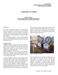
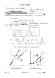
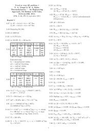
Figure 1 shows a combustor and the main airflows within. Fuel
is supplied through the fuel injector and initially mixed together
with only a part of the inlet airflow. Some of the cold airflow is
supplied through the liner wall continuous along the combustor
length to achieve a satisfying combustion and to cool the liner
wall. The rest of the cold airflow, if no air for blade cooling is
needed, is mixed together with the hot gas at the outlet of the
combustor to achieve an acceptable temperature profile which
fulfills the demands for the turbine inlet.
Figure 1 (Genrup, 2012)
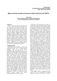
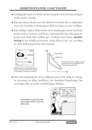
Figure 2 shows components of the heat flux in an element of
the liner wall (1).
Copyright © 2012 by William Wiberg

In real application the liner wall can’t be seen as a black body
and Lefebvre (1) suggested that introducing the factor
0.5(1+ε w ) into Eq. 3 should compensate for that effect. Further,
Lefebvre suggests that the ratio
α g
ε g
= T g
T w 1
1.5
is a valid approximation. With these assumptions Eq. 3 can be
written as
Figure 2
With direction of the fluxes as in Figure 2 and with the
assumption that the liner wall is thin (A inner ≈ A outer ), heat
balance of the marked element can be written as
R 1 + C 1 + K = K 1−2 = C 2 + R 2 Eq. 1
The problem to determine the thermal load at the liner wall then
comes down approximate these components.
There are two major approaches to evaluate the fluxes as shown
in Figure 2, either by empirical correlations or by numerical
methods.
LITERATURE SURVEY
The heat transfer in gas turbine combustor has been subject to
many research projects and, due to the complex phenomena of
chemical reactions, turbulent flow and heat transfer, still is.
Lefebvre’s and Ballal’s (1) work address many empirical
correlations to describe the heat transfer in different types of
combustion. Bahador. M (Mehdi, 2007) has done a doctoral
thesis on the subject with focus on how to model the radiative
heat transfer. The doctoral thesis covers both empirical and
numerical methods, where the empirical methods mostly are a
summery of Lefebvre’s work.
PROJECT DESCRIPTION
The empirical approach
As described in Lefebvre’s work (1) can the contribution from
the conduction K in Figure 2 always be neglected compared to
the other components and Eq. 1 is then reduced to
R 1 + C 1 = K 1−2 = C 2 + R 2
The conduction through the liner wall can be described as
K 1−2 = k w
t w
(T w1 − T w2 ) Eq. 2
If the inner liner wall is considered as a black body the net
internal radiation is (2)
R 1 = ε g ςT g 4 − α g ςT w1
4
Eq. 3
R 1 = 0.5 1 + ε w ε g T g 1.5 (T g 2.5 − T w1 2.5 ) Eq. 4
According to Lefebvre (1), the heat transferred by radiation can
be divided into two components, non-luminous and luminous
gases. The contribution from the different components can be
brought into the equation by evaluate the gas emissivity as
ε g = 1 − exp⁡[−290PL(ql b ) 0.5 T g −1.5 ]
Where P is the pressure, L the luminosity factor, q the air to fuel
ratio, l b the beam length and T g the hot gas temperature.
Lefebvre (1) presented a correlation for the luminosity factor L
according to
L = 336
H 2
where H is the hydrogen content in the fuel in mass percent.
The radiation from the outer liner wall to the casing is
described as radiation between two gray bodies according to
Lefebvre (1) and can, if respectively wall temperature is
assumed to be constant in axial direction, be formulated as
ς(T 4 w2 − T 4 c )
R 2 A w =
1 − ε w
+ 1 + 1 − ε c Eq. 5
ε w A w A w F wc ε c A c
Further simplifications can be made with additional
assumptions and Lefebvre proposes following simplification of
Eq. 5 for aluminum respectively steel casing
and
R 2 = 0.4 ς(T w2 4 − T 3 4 )
R 2 = 0.6 ς(T w2 4 − T 3 4 )
The heat transferred to and from the liner wall due to
convection is
C 1 = 1 (T g − T w1 ) Eq. 6
and
C 2 = 2 (T w2 − T a ) Eq. 7
Copyright © 2012 by William Wiberg

The challenge is to find an acceptable approximation of the
heat transfers coefficients 1 and 2 , which of course is
troublesome due to the complex flow and the chemical
conditions, especially in the primary zone. Lefebvre (1) makes
the assumption that the convective heat transfer in a combustor
has sufficiently similarities with the convective heat transfer in
a pipe to be treated accordingly. The internal convection can
then be described as
C 1 = 0.020
k g m 0.8
g
0.2
(T
D L
A L μ g − T w1 ) Eq. 8
g
where D L is the hydraulic diameter of the liner. For the
convective heat transfer in the primary zone the factor 0.020
can be set to 0.017 to compensate for a somewhat lower bulk
temperature T g . The external convection is, with the same
treatment, described as
C 2 = 0.020
k a m 0.8
a
0.2
(T
D an
A an μ w2 − T a ) Eq. 9
a
where D an is the hydraulic diameter of the annulus air space.
All these expressions can be brought back into Eq. 1 from
which the wall temperatures T w1 and T w2 can be calculated.
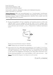
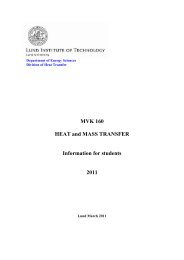
However, if the liner wall is treated with some kind of filmcooling
method, as is common in most combustors today,
corrections to the expressions for the internal convection C 1
have to be made. A schematic figure of the film-cooling process
is shown in Figure 3.
η = T g − T w ,ad
T g − T a
where T w ,ad is the adiabatic wall temperature. T w,ad is then
used to calculate the convective heat transfer, as proposed by
Lefebvre (1), accordingly to
C 1 = 0.069 k a
x Re x 0.7 (T w ,ad − T w1 ) if 0.5 < m < 1.3
C 1 = 0.10 k a
x Re x 0.8
where is m = (Uρ ) a
(Uρ ) g
.
x
s
−0.36
(Tw ,ad − T w1 ) if 0.5 < m < 1.3
The adiabatic wall temperature is calculated from the filmcooling
effectiveness. Dependent of the ratio between the
cooling air stream velocity and the main stream velocity the
boundary layer downstream the cooling slot is treated in two
different ways, by the Turbulent boundary layer model for
modest ratio or by the Wall-jet model when the cooling air
stream velocity is much greater than the main stream velocity.
Expressions for the film-cooling effectiveness for the different
models are further investigated by Lefebvre (1).
The numerical approach
Whereas empirical methods give a quick and initially good
approximation of what average temperatures to expect in the
combustor, they lack in detail and precision. With valid
mathematical models of the processes that occur in the
combustor, the possibility to more precisely describe the
phenomena increases with the available computational power.
The governing equations of interest is presented by Bahador (3)
as
∂ρ
Continuity:
∂t + ∂ρu i
= 0
∂x i
Momentum:
Energy:
∂ρu i
∂t
+ ∂ρu j u i
∂x j
= − ∂p
∂x i
+ ∂τ ij
∂x j
∂ρ
∂t + ∂ρu i
= ∂p
∂x i ∂t + u ∂p
i − ∂q i ∂u i
+ τ
∂x i ∂x ij + S
i ∂x q
j
Species:
∂ρY k
∂t
+ ∂ρu iY k
∂x i
= − ∂ρV i,kY k
∂x i
+ ω k (k = 1, . . , N)
Figure 3 (1)
To take account for the cooling effect a film-cooling
effectiveness is defined as
where
and
τ ij = 2μS ij − 2 μ∂u k
δ
3 ∂x ij Eq. 10
k
Copyright © 2012 by William Wiberg

q i = −k ∂T
∂x i
+ ρ
N
k=1
k Y k V i,k
Eq. 11
The heat source term in the energy equation is, with the thermal
radiation conditions in a combustor, given by
S q = −∇q r (r) Eq. 12
Where the divergence of the radiative heat flux is derived from
the radiative transfer equation (RTE) as done by Bahador (3)
and can be written as
−∇q r r = κ r (4πI b r − G(r)) Eq. 13
Further details regarding the RTE can be found in reference (3)
and (4). To solve Eq. 13 in any real application one has to rely
on numerical approximations. Bahador (3) suggests either the
Discrete Ordinates Method (DOM) or the Finite Volume
Method (FMV) but other possibilities are available such as the
Spherical Harmonics Method (P N -approximation) and the
Zonal Method.
In addition to the special treatment of the radiative heat flux
some model is needed to take the turbulent flow into account.
Normally the Reynolds averaged Navier-Stokes (RANS) model
or Large Eddy Simulation (LES) is used in the industry. For
research purposes or if a fully resolved flow field is required
the Direct Numerical Simulation (DNS) may be used. For more
details regarding turbulence modeling the reader is referred to
CFD-literature.
Another troublesome process to model is the combustion
process, represented by the reaction rate ω k in the conservation
of species equation. A mean reaction rate model is presented by
Bahador (3) and defined as
q ′′ = T w − T f − q rad ′′ Eq. 155
CONCLUSIONS
The empirical and numerical approach to predict the liner wall
temperature both has its advantages and disadvantages and one
may argue that one of them cannot fully replace the other. As
far as local accuracy goes, the numerical methods gives a much
better approximation, even though improvements regarding the
modeling of the more complex physical and chemical processes
is desirable. The drawback is of course the computational
power and time required to get an acceptable result, whereas
empirical correlations gives a quick, but nonetheless useful,
result even by hand calculation. Whether numerical methods
give better results than empirical is of course a question about
the requirements of the accuracy. In an initial design stage of a
combustor, empirical correlations probably provides a sufficient
prediction of the thermal load whereas in later stages, if more
detailed data is required, a numerical analysis provides more
information.
REFERENCES
1. Lefebvre, Arthur and Ballal, Dilip. Gas Turbine
Combustion. s.l. : CRC Press, 2010.
2. Sundén, Bengt. Värmeöverföring. Lund : Studentlitteratur,
2006.
3. Bahador, Mehdi. On Radiative Heat Transfer Modeling with
Relevance for Combustors and Biomass Furnaces. Department
of Energy Sciences, Lund Institue of Technology. Lund : Lund
Institue of Technology, 2007. Doctoral Thesis.
4. Yuan, Jinliang. Heat and Mass Transfer. Lund : Department
of Energy Sciences, 2012.
5. Saravanamuttoo, HH, et al. Gas Turbine Theory.
Edinburgh Gate, England : Pearson Education Limited, 2009.
6. Genrup, Magnus. Lund : Lund University, 2012.
ω k = − ρ A EDM
t T
where A EDM and B EDM are constants and
min⁡(Y f , Y o
s o
, B EDM
Y P
s P
) Eq. 14
s o = oxygen
fuel
stoic
, s p = products
fuel
stoic
where the ratios are based by mass.
This model is suitable for both premixed and diffusion flames.
Even though there are models for the reaction rate, the process
of soot-formation in a turbulent flame is still rather unresolved.
The formation of soot is a process which greatly influences the
radiative heat flux.
When appropriate numerical treatment of the radiative heat flux
and turbulence model is chosen, the local wall temperature for
each point can be solved from
Copyright © 2012 by William Wiberg