About a dynamic model of interaction of insect population with food ...
About a dynamic model of interaction of insect population with food ...
About a dynamic model of interaction of insect population with food ...

You also want an ePaper? Increase the reach of your titles
YUMPU automatically turns print PDFs into web optimized ePapers that Google loves.
Computational Ecology and S<strong>of</strong>tware, 2011, 1(4):208-217<br />
Article<br />
<strong>About</strong> a <strong>dynamic</strong> <strong>model</strong> <strong>of</strong> <strong>interaction</strong> <strong>of</strong> <strong>insect</strong> <strong>population</strong> <strong>with</strong> <strong>food</strong> plant<br />
L.V. Nedorezov<br />
The Research Center for Interdisciplinary Environmental Cooperation (INENCO) <strong>of</strong> Russian Academy <strong>of</strong> Sciences, Kutuzova<br />
nab. 14, 191187 Saint-Petersburg, Russia<br />
E-mail: l.v.nedorezov@gmail.com<br />
Received 13 July 2011; Accepted 16 August 2011; Published online 1 December 2011<br />
IAEES<br />
Abstract<br />
In present paper there is the consideration <strong>of</strong> mathematical <strong>model</strong> <strong>of</strong> <strong>food</strong> plant (resource) – consumer (<strong>insect</strong><br />
<strong>population</strong>) – pathogen system <strong>dynamic</strong>s which is constructed as a system <strong>of</strong> ordinary differential equations.<br />
The <strong>dynamic</strong> regimes <strong>of</strong> <strong>model</strong> are analyzed and, in particular, <strong>with</strong> the help <strong>of</strong> numerical methods it is shown<br />
that trigger regimes (regimes <strong>with</strong> two stable attractors) can be realized in <strong>model</strong> under very simple<br />
assumptions about ecological and intra-<strong>population</strong> processes functioning. Within the framework <strong>of</strong> <strong>model</strong> it<br />
was assumed that the rate <strong>of</strong> <strong>food</strong> flow into the system is constant and functioning <strong>of</strong> intra-<strong>population</strong> selfregulative<br />
mechanisms can be described by Verhulst <strong>model</strong>. As it was found, trigger regimes are different <strong>with</strong><br />
respect to their properties: in particular, in <strong>model</strong> the trigger regimes <strong>with</strong> one <strong>of</strong> stable stationary points on the<br />
coordinate plane can be realized (it corresponds to the situation when sick individuals in <strong>population</strong> are absent<br />
and their appearance in small volume leads to their asymptotic elimination); also the regimes <strong>with</strong> several nonzero<br />
stationary states and stable periodic fluctuations were found.<br />
Keywords <strong>population</strong> <strong>dynamic</strong>s; mathematical <strong>model</strong>; trigger regimes; <strong>insect</strong> <strong>population</strong> outbreak.<br />
1 Introduction<br />
In modern literature it is possible to find a lot <strong>of</strong> various publications that are devoted to the analysis <strong>of</strong><br />
resource-consumer system <strong>dynamic</strong>s (see, for example, Varley et al., 1973; Smith, 1974; Berryman, 1981,<br />
1982; Nedorezov, 1986; Berryman et al., 1987; and others). Formally, we can also consider the predator-prey<br />
system as a resource-consumer system. In both situations we have the <strong>interaction</strong> <strong>of</strong> two species, which belong<br />
to various trophic levels. On the other hand, in <strong>interaction</strong> between forest <strong>insect</strong>s and its <strong>food</strong> plants it is<br />
possible to point out several specific features which can’t be observed in <strong>interaction</strong> between <strong>population</strong>s <strong>of</strong><br />
animals (see, for example, Isaev et al, 1984, 2001, 2009; Nedorezov and Utyupin, 2011). In particular,<br />
<strong>interaction</strong> between fir beetle (Monochamus urussovi Fisch.) <strong>with</strong> <strong>food</strong> plant (fir Abies sibirica) leads to the<br />
realization <strong>of</strong> the following effect: increasing <strong>of</strong> <strong>population</strong> size leads to the increasing <strong>of</strong> the volume <strong>of</strong> <strong>food</strong><br />
(which is suitable for larva eating) in system (Isaev et al, 1984, 2001). The similar effect is typical for<br />
Xylotrechus altaicus Gebl. (Rozhkov, 1982) and for Protocryptis sibiricella Falk. (Ermolaev, 2011a, 2011b)<br />
<strong>with</strong> <strong>interaction</strong> <strong>of</strong> these species <strong>with</strong> Larix sibirica.<br />
Analysis <strong>of</strong> two-component (<strong>insect</strong> <strong>population</strong> – <strong>food</strong> plants) system <strong>dynamic</strong>s <strong>with</strong>in the framework <strong>of</strong> nonparametric<br />
system <strong>of</strong> ordinary differential equations (<strong>model</strong> <strong>of</strong> Kolmogorov’ type; Kolmogor<strong>of</strong>f, 1937)<br />
showed (Isaev et al, 2009; Nedorezov, 1986, 1997) that at positive feedback in this relation the regimes <strong>of</strong><br />
IAEES<br />
www.iaees.org
Computational Ecology and S<strong>of</strong>tware, 2011, 1(4):208-217<br />
209<br />
various modifications <strong>of</strong> fixed outbreak can only be realized (<strong>population</strong> size can be stabilized at one <strong>of</strong> two<br />
various stable levels). And this result corresponds to considering in boreal forests fluctuations <strong>of</strong> Monochamus<br />
urussovi Fisch. and Xylotrechus altaicus Gebl. <strong>population</strong>s (Isaev et al, 1984, 2001, 2009; Rozhkov, 1982). If<br />
negative feedback is observed in <strong>insect</strong> – <strong>food</strong> plant system all types <strong>of</strong> mass propagations <strong>of</strong> forest <strong>insect</strong>s can<br />
be realized <strong>with</strong>in the framework <strong>of</strong> non-parametric <strong>model</strong> (Nedorezov, 1986, 1997).<br />
Epizootics, which are arose in <strong>insect</strong> <strong>population</strong>s, for example, at any critical <strong>population</strong> levels, play very<br />
important regulative role in <strong>population</strong> <strong>dynamic</strong>s (Berryman, 1981, 1982; Varley et al., 1973; Isaev et al, 1984,<br />
2001, 2009; Vorontsov, 1963, 1978; Isaev and Girs, 1975). Some authors assume that epizootics can play the<br />
most important role in development <strong>of</strong> any types <strong>of</strong> mass propagations <strong>of</strong> forest <strong>insect</strong>s (Berryman, 1981, 1982;<br />
Berryman et al., 1987; Konikov, 1978). For some particular cases this opinion is supported by the analysis <strong>of</strong><br />
mathematical <strong>model</strong>s (Nedorezov, 1986, 1997; Nedorezov and Utyupin, 2011).<br />
Up to current time moment the problem about combined influence <strong>of</strong> epizootics and <strong>food</strong> plants onto forest<br />
<strong>insect</strong> <strong>population</strong> <strong>dynamic</strong>s is open. One <strong>of</strong> the main questions <strong>of</strong> analysis <strong>of</strong> this situation is following: what<br />
kind <strong>of</strong> types <strong>of</strong> <strong>insect</strong> outbreaks can be realized at combined influence <strong>of</strong> these regulators? And what are the<br />
conditions for realization <strong>of</strong> outbreak regimes?<br />
In current publication we analyze some particular cases <strong>of</strong> this problem. Analysis <strong>of</strong> non-parametric <strong>model</strong>s<br />
in multi-dimensional situation has a lot <strong>of</strong> serious problems; at the same time analysis <strong>of</strong> parametric <strong>model</strong>s<br />
(<strong>model</strong>s <strong>of</strong> Volterra’s type; Volterra, 1931; Nedorezov, 2011) doesn’t allow obtaining the whole spectra <strong>of</strong><br />
<strong>dynamic</strong> regimes, which can be realized in considering system. But some basic regimes, which are typical for<br />
considering situation, can be obtained <strong>with</strong>in the framework <strong>of</strong> parametric <strong>model</strong>.<br />
2 Description <strong>of</strong> Model<br />
Let x (t)<br />
be the number <strong>of</strong> healthy individuals in a <strong>population</strong>, y (t)<br />
be the number <strong>of</strong> sick individuals, and<br />
P (t) be the volume <strong>of</strong> suitable <strong>food</strong> for consumption in a system at time t .<br />
Let’s assume that the following processes have the direct influence on the <strong>dynamic</strong>s <strong>of</strong> variable x (t)<br />
:<br />
natural birth process and natural death process <strong>of</strong> individuals (<strong>with</strong> an intensity <br />
x<br />
; <strong>with</strong>in the framework <strong>of</strong><br />
<strong>model</strong> we shall assume that the amount <strong>of</strong> this intensity <br />
x<br />
depends on the relation <strong>of</strong> numbers <strong>of</strong> <strong>population</strong><br />
groups x (t)<br />
and y (t)<br />
, and volume <strong>of</strong> <strong>food</strong> P (t)<br />
), intra-<strong>population</strong> competition between individuals (<strong>with</strong><br />
positive coefficient <br />
x<br />
), and <strong>interaction</strong> between healthy and sick individuals that leads to the decreasing <strong>of</strong><br />
number <strong>of</strong> healthy individuals <strong>with</strong> the rate <br />
x<br />
xy , <br />
x<br />
const 0 (that corresponds to the “principle <strong>of</strong> pair<br />
<strong>interaction</strong>” by V. Volterra, 1931). It is very important to note that <strong>with</strong>in the framework <strong>of</strong> considering <strong>model</strong><br />
we don’t take into account the possibility <strong>of</strong> appearance <strong>of</strong> sick individuals in <strong>population</strong> as a result <strong>of</strong> very<br />
high concentration <strong>of</strong> individuals. It can realize, for example, on the peak phase <strong>of</strong> <strong>insect</strong> outbreak<br />
development (Isaev et al., 1984, 2001, 2009).<br />
Dynamics <strong>of</strong> variable y (t)<br />
is determined by the influence <strong>of</strong> the following processes: natural death <strong>of</strong><br />
individuals (<strong>with</strong> an intensity <br />
y<br />
; in <strong>model</strong> we shall assume that the value <strong>of</strong> this coefficient depends on the<br />
relation <strong>of</strong> numbers <strong>of</strong> <strong>population</strong> groups x (t)<br />
and y (t)<br />
, and volume <strong>of</strong> suitable <strong>food</strong> P (t)<br />
), intra-<strong>population</strong><br />
competition between individuals (<strong>with</strong> positive coefficient <br />
y<br />
), and inflow <strong>of</strong> new sick individuals which<br />
appear in a result <strong>of</strong> <strong>interaction</strong> between sick and healthy individuals (<strong>with</strong> the rate <br />
x<br />
xy ).<br />
Let’s also assume that <strong>dynamic</strong>s <strong>of</strong> variable P (t)<br />
is determined by the influence <strong>of</strong> following processes:<br />
inflow into the system <strong>of</strong> suitable <strong>food</strong> <strong>with</strong> the rate P 0<br />
(<strong>with</strong>in the framework <strong>of</strong> considering <strong>model</strong> it is<br />
assumed that this rate is constant; in general case the amount <strong>of</strong> this rate depends on the level <strong>of</strong> influence <strong>of</strong><br />
<strong>insect</strong>s onto the <strong>food</strong> plant; Isaev and Girs, 1975), flow <strong>of</strong> <strong>food</strong> out <strong>of</strong> the system that doesn’t depend on the<br />
IAEES<br />
www.iaees.org
210<br />
Computational Ecology and S<strong>of</strong>tware, 2011, 1(4):208-217<br />
<strong>interaction</strong> between <strong>insect</strong> <strong>population</strong> and <strong>food</strong> plants (<strong>with</strong> an intensity <br />
p<br />
), and, respectively, outflow <strong>of</strong><br />
<strong>food</strong> that correlates <strong>with</strong> influence <strong>of</strong> <strong>insect</strong>s onto <strong>food</strong> plants (<strong>with</strong> coefficient <br />
p<br />
).<br />
Taking into account all assumptions about the basic processes in considering system made above, we have<br />
the following system <strong>of</strong> ordinary differential equations:<br />
dx<br />
dt<br />
dy<br />
x x( x y)<br />
xy ,<br />
x<br />
x<br />
x<br />
<br />
x<br />
xy <br />
y<br />
y( x y)<br />
<br />
y<br />
y ,<br />
dt<br />
dP<br />
P0 <br />
p<br />
P <br />
p<br />
P(<br />
x y)<br />
, (1)<br />
dt<br />
where parameter describes the inequality <strong>of</strong> influence <strong>of</strong> sick and healthy individuals onto <strong>food</strong> plants (note,<br />
that sick individuals need in bigger volume <strong>of</strong> <strong>food</strong>, and, thus, we have const 1).<br />
Let c<br />
1<br />
and c<br />
2<br />
be the parameters, which are equal to the rates <strong>of</strong> <strong>food</strong> consumption by healthy and sick<br />
individuals respectively (for example, grams per day, grams per hour etc.). Thus, the difference<br />
c x c y P corresponds to <strong>food</strong> conditions in the system at every time moment. If 0 it means<br />
<br />
1 2<br />
that in the system there is enough big volume <strong>of</strong> <strong>food</strong> and competition between individuals for <strong>food</strong> is absent.<br />
At realization <strong>of</strong> this inequality it is naturally to assume that death rates don’t depend on the value <strong>of</strong> : at<br />
0<br />
0<br />
0 Malthusian parameters in system (1) are constant, <br />
x<br />
x<br />
и <br />
y<br />
y<br />
, 0 x<br />
0 , 0 y<br />
0 .<br />
Consequently, in domain 0 <strong>dynamic</strong>s <strong>of</strong> considering system will describe by the following differential<br />
equations:<br />
dx<br />
dt<br />
dy<br />
0<br />
x x(<br />
x y)<br />
xy ,<br />
x<br />
x<br />
0<br />
<br />
x<br />
xy <br />
y<br />
y( x y)<br />
<br />
y<br />
y ,<br />
dt<br />
dP<br />
P0 <br />
p<br />
P <br />
p<br />
P(<br />
x y)<br />
, (2)<br />
dt<br />
If 0 in the system there is not sufficient volume <strong>of</strong> <strong>food</strong> and, respectively, in this situation there exists<br />
intra-<strong>population</strong> competition between individuals for <strong>food</strong>. For this situation we’ll assume that amounts <strong>of</strong><br />
Malthusian parameters can be described as following linear functions:<br />
0 1<br />
0 1<br />
<br />
x<br />
<br />
x<br />
<br />
x<br />
, <br />
y<br />
<br />
y<br />
<br />
y<br />
,<br />
where 1 x<br />
0 , 1 y<br />
0 are non-negative parameters. Respectively, if 0 <strong>dynamic</strong>s <strong>of</strong> considering<br />
system is described by the following system <strong>of</strong> differential equations:<br />
dx<br />
dt<br />
dy<br />
0 1<br />
x <br />
x c x c y P)<br />
x(<br />
x y)<br />
xy ,<br />
x<br />
x<br />
(<br />
1 2<br />
0 1<br />
<br />
x<br />
xy <br />
y<br />
y( x y)<br />
<br />
y<br />
y <br />
y<br />
y(<br />
c1x<br />
c2<br />
y P)<br />
,<br />
dt<br />
dP<br />
P0 <br />
p<br />
P <br />
p<br />
P(<br />
x y)<br />
. (3)<br />
dt<br />
x<br />
x<br />
x<br />
IAEES<br />
www.iaees.org
Computational Ecology and S<strong>of</strong>tware, 2011, 1(4):208-217<br />
211<br />
Remark. It is also possible to assume that increase <strong>of</strong> values <strong>of</strong> leads to the decrease <strong>of</strong> the intensity <strong>of</strong> birth<br />
rate. And it seems rather natural that decrease <strong>of</strong> this intensity <strong>of</strong> <strong>population</strong> growth can be described by<br />
exponential function.<br />
3 Properties <strong>of</strong> Model (2)-(3)<br />
(1) There exists a stable invariant compact set in non-negative part <strong>of</strong> phase space; trajectories <strong>of</strong> system <strong>of</strong><br />
ordinary differential equations (2)-(3) can’t intersect the boundaries <strong>of</strong> this compact set:<br />
0, x ] [0,<br />
y ] [0,<br />
P ],<br />
where<br />
[<br />
max<br />
max<br />
max<br />
P0<br />
Pmax ,<br />
<br />
p<br />
0<br />
x<br />
xmax ,<br />
<br />
x<br />
y<br />
max<br />
<br />
x<br />
xmax<br />
<br />
y<br />
<br />
0<br />
y<br />
.<br />
It means that for every non-negative initial values <strong>of</strong> <strong>model</strong> variables, <strong>population</strong> size and volume <strong>of</strong> <strong>food</strong> in<br />
the system are non-negative and bounded for every time moment t 0 .<br />
(2) If initial value y<br />
0<br />
0 (this is the situation when we have no sick individuals in the system at initial time<br />
moment) all trajectories <strong>of</strong> <strong>model</strong> (2)-(3) belong to coordinate plane y 0 . It means that if the number <strong>of</strong> sick<br />
individuals at initial time moment is equal to zero it would be equal to zero for every time moment t 0 (as it<br />
was pointed out above this property doesn’t realize in common situation – if number <strong>of</strong> healthy individuals is<br />
greater than certain level, sick individuals can appear in the system, for example, in a result <strong>of</strong> over<br />
concentration <strong>of</strong> individuals).<br />
If initial value x<br />
0<br />
0 (there are no healthy individuals in the system at initial time moment) trajectories <strong>of</strong><br />
<strong>model</strong> (2)-(3) belong to coordinate plane x 0 . It means that if x<br />
0<br />
0 the number <strong>of</strong> healthy individuals in<br />
the system will be equal to zero for every time moments t 0 . Taking into account all assumptions made<br />
above, in this situation <strong>population</strong> eliminates at all possible values <strong>of</strong> other variables <strong>of</strong> <strong>model</strong> (2)-(3). In other<br />
words, all trajectories converge to stationary state ( 0,0, P<br />
0<br />
/ <br />
2<br />
) asymptotically. Also it means that this<br />
stationary point ( 0,0, P<br />
0<br />
/ <br />
2<br />
) can be a stable knot (in particular, when intensity <strong>of</strong> birth rate is less than<br />
intensity <strong>of</strong> death rate <strong>of</strong> individuals) or saddle point (plane x 0 is a surface <strong>of</strong> incoming separatrixes; in all<br />
cases axis P is incoming integral curve).<br />
(3) Stationary states <strong>of</strong> <strong>model</strong> in the domain 0 .<br />
We’ll assume that coefficients <strong>of</strong> self-regulation x<br />
and <br />
y<br />
are positive, <br />
x<br />
, <br />
y<br />
const 0 , and<br />
<strong>population</strong> doesn’t eliminate for all initials values <strong>of</strong> variables. In this case in <strong>model</strong> the following stationary<br />
states can appear:<br />
(3.1) Point 0,<br />
0, P0 / p<br />
is unstable stationary state (a saddle point; out-coming separatrix belongs to plane<br />
y 0 ). Note, that for all possible values <strong>of</strong> <strong>model</strong> parameters this equilibrium point belongs to the domain<br />
0 . Thus, for all possible sufficient small initial values <strong>of</strong> healthy individuals x<br />
0<br />
0 <strong>model</strong> trajectories<br />
go out <strong>of</strong> this stationary state; if and only if initial number <strong>of</strong> healthy individuals is equal to zero trajectory<br />
asymptotically converges to this stationary point (<strong>population</strong> eliminates and volume <strong>of</strong> <strong>food</strong> stabilizes at<br />
constant level P0 / <br />
p<br />
). There are no other stationary states, which belong to coordinate lines.<br />
IAEES<br />
www.iaees.org
212<br />
Computational Ecology and S<strong>of</strong>tware, 2011, 1(4):208-217<br />
Let’s denote as R ( 1<br />
R1 x,<br />
y,<br />
P)<br />
, R (<br />
2<br />
R2 x,<br />
y,<br />
P)<br />
, and R3 R3(<br />
x,<br />
y,<br />
P)<br />
the right-hand sides <strong>of</strong><br />
equations <strong>of</strong> <strong>model</strong> (2)-(3) for variables x , y , and P respectively. For equations (2) we have the following<br />
relations:<br />
R<br />
x<br />
1<br />
0<br />
<br />
x<br />
2<br />
x<br />
x <br />
x<br />
y <br />
x<br />
y , R 1 <br />
x<br />
x x<br />
x<br />
y<br />
, R<br />
1<br />
<br />
P<br />
0 ;<br />
R 2 <br />
y<br />
y <br />
x<br />
y<br />
x<br />
,<br />
R<br />
y<br />
2<br />
x <br />
x<br />
0<br />
2<br />
y<br />
y <br />
y<br />
x <br />
y<br />
R<br />
, 2<br />
0 ;<br />
P<br />
R 3 P<br />
P<br />
x<br />
, R 3 <br />
y<br />
P P<br />
<br />
<br />
, R3<br />
<br />
( x y<br />
P<br />
)<br />
p<br />
<br />
P<br />
.<br />
<br />
The Jacobian matrix calculating in point 0,<br />
0, P0 / p<br />
for the system (2) has the following form:<br />
<br />
<br />
<br />
<br />
0<br />
<br />
x<br />
0 0<br />
<br />
<br />
<br />
P0<br />
<br />
0<br />
J 0 , 0, 0 <br />
y<br />
0 .<br />
<br />
<br />
<br />
p <br />
<br />
p<br />
P0<br />
<br />
pP0<br />
<br />
<br />
<br />
p <br />
<br />
p<br />
<br />
p <br />
Thus, we have the following result: if 0 x<br />
0<br />
(3.2) Stationary state<br />
stationary state , 0, / <br />
0 P0 p<br />
is unstable saddle point.<br />
<br />
<br />
0<br />
<br />
x<br />
, 0,<br />
<br />
<br />
x<br />
<br />
p<br />
<br />
<br />
<br />
P0<br />
<br />
0 <br />
<br />
p<br />
x<br />
<br />
<br />
x <br />
corresponds to the situation when there are no sick individuals in the system. Let<br />
P<br />
*<br />
P<br />
P<br />
0<br />
x 0<br />
<br />
.<br />
0<br />
0<br />
<br />
p<br />
x<br />
<br />
p<br />
x<br />
<br />
p<br />
x<br />
<br />
p<br />
<br />
<br />
x<br />
If the following inequality is truthful<br />
c <br />
1<br />
<br />
x<br />
0<br />
x<br />
*<br />
P ,<br />
IAEES<br />
www.iaees.org
Computational Ecology and S<strong>of</strong>tware, 2011, 1(4):208-217<br />
213<br />
or<br />
c<br />
0<br />
0<br />
2<br />
1<br />
<br />
x<br />
( <br />
p<br />
x<br />
<br />
p<br />
x<br />
) P0<br />
<br />
x<br />
, (4)<br />
this point belongs to the domain 0 . If the inverse inequality is realized in (4) for <strong>model</strong> parameters this<br />
point must belong to the domain 0 (but in this situation we have to recalculate point’s coordinates using<br />
equations (3)). The Jacobian matrix calculating in considering point for the system (2) has the following form:<br />
0<br />
<br />
0 <br />
<br />
x<br />
( <br />
x<br />
<br />
x<br />
)<br />
<br />
<br />
x<br />
<br />
0<br />
<br />
<br />
x<br />
<br />
0 <br />
0<br />
<br />
<br />
<br />
<br />
x<br />
( <br />
x<br />
<br />
y<br />
)<br />
x *<br />
0<br />
J<br />
, 0, P <br />
0 <br />
<br />
<br />
y<br />
0 .<br />
<br />
x <br />
<br />
x<br />
<br />
<br />
0<br />
<br />
p<br />
*<br />
*<br />
x<br />
<br />
<br />
<br />
<br />
<br />
p<br />
P <br />
pP<br />
<br />
p<br />
<br />
<br />
x <br />
Thus, we have the following characteristic values:<br />
<br />
,<br />
0<br />
1 x<br />
<br />
2<br />
0<br />
<br />
x<br />
( <br />
x<br />
<br />
y<br />
)<br />
0<br />
<br />
y<br />
<br />
<br />
<br />
,<br />
x<br />
<br />
3<br />
<br />
p<br />
<br />
<br />
p<br />
<br />
<br />
x<br />
0<br />
x<br />
.<br />
Taking into account that<br />
1<br />
, 0<br />
3<br />
<br />
inequality is observed for <strong>model</strong> parameters:<br />
, considering point is a stable equilibrium <strong>of</strong> the system if the following<br />
0<br />
( )<br />
0 x<br />
<br />
x<br />
<br />
y<br />
<br />
y<br />
<br />
0 . (5)<br />
<br />
x<br />
This point is unstable equilibrium if in (5) we have the inverse inequality. On the coordinate plane y 0<br />
(when there are no sick individuals in the system) this point is global stable knot. There are no other stationary<br />
points on coordinate planes.<br />
(3.3) Let<br />
0<br />
<br />
x<br />
<br />
y<br />
A <br />
<br />
0<br />
y<br />
<br />
y<br />
x<br />
0<br />
y<br />
x<br />
0 ,<br />
Stationary point x<br />
** ** **<br />
, y , P<br />
<br />
<br />
x<br />
y<br />
( <br />
x<br />
<br />
y<br />
)( <br />
x<br />
<br />
x<br />
)<br />
B .<br />
<br />
, where<br />
y<br />
IAEES<br />
www.iaees.org
214<br />
Computational Ecology and S<strong>of</strong>tware, 2011, 1(4):208-217<br />
x<br />
**<br />
<br />
A<br />
B<br />
,<br />
y<br />
<br />
x<br />
<br />
**<br />
y<br />
)<br />
** 0<br />
( x <br />
y<br />
,<br />
<br />
y<br />
P<br />
**<br />
P0<br />
,<br />
** **<br />
( x y<br />
)<br />
p<br />
p<br />
exists if the following inequalities are realized:<br />
** 0<br />
0 , ( <br />
x<br />
<br />
y<br />
) x <br />
y<br />
0 . (6)<br />
x<br />
x<br />
y<br />
Taking into account that point’s coordinates must be positive the first inequality in (6) can be omitted. It is<br />
obvious, that two first equations for variables x and y <strong>of</strong> the system (2) don’t depend on third equation. Thus,<br />
analysis <strong>of</strong> the behaviour <strong>of</strong> trajectories on the plane ( x , y)<br />
can give us basic properties <strong>of</strong> non-trivial<br />
stationary state. Trajectories on the plane ( x , y)<br />
are bounded. Use <strong>of</strong> Dulac criteria (Andronov et al., 1959)<br />
<strong>with</strong> function 1/(<br />
xy ) allows us to prove that in positive part <strong>of</strong> the plane ( x , y)<br />
there are no limit cycles.<br />
Thus, unique non-trivial stationary state is global (on the plane) stable equilibrium. Consequently, point<br />
** ** **<br />
x , y , P in the domain 0 is asymptotically stable. It also means that we cannot have limit cycles<br />
which belongs to the domain 0 only.<br />
(4) Stationary states in the domain 0 . It is obvious that number <strong>of</strong> non-trivial stationary states in this<br />
domain is less or equal to two.<br />
(5) Numerical experiments. Provided calculations showed that <strong>with</strong>in the framework <strong>of</strong> <strong>model</strong> (2)-(3) the<br />
following <strong>dynamic</strong> regimes could be realized:<br />
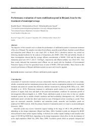
Fig. 1 Changing <strong>of</strong> stationary level P <strong>of</strong> variable (t)<br />
determined by the equation (7).<br />
P at increase <strong>of</strong> <strong>food</strong> flow into the system P<br />
0 (blue line). Red line is<br />
(5.1) Regime <strong>with</strong> unique global stable state in phase space (all variables converge to this equilibrium<br />
asymptotically at non-zero initial values). This equilibrium can belong as to domain 0 , as to domain<br />
IAEES<br />
www.iaees.org
Computational Ecology and S<strong>of</strong>tware, 2011, 1(4):208-217<br />
215<br />
0 . On Fig. 1 the changing <strong>of</strong> stationary value P <strong>of</strong> P (t)<br />
at increase <strong>of</strong> speed flow <strong>of</strong> <strong>food</strong> into the<br />
system P<br />
0<br />
is presented (blue line). The red line on this fig. 1 is determined by the following equation:<br />
c x c y , (7)<br />
P<br />
1<br />
<br />
2<br />
where x and y are the stationary levels <strong>of</strong> the respective variables <strong>of</strong> the <strong>model</strong>. This picture was obtained<br />
for the following values <strong>of</strong> <strong>model</strong> parameters: c 0. 1<br />
004 , c 1. 1 2 , 0. 15<br />
p<br />
, 0 x<br />
80 , 1 x<br />
5 ,<br />
<br />
x<br />
0.01 , <br />
x<br />
10 , <br />
y<br />
0. 5 , 0 y<br />
0. 1, <br />
p<br />
0. 0009 , 60 , 1 y<br />
7 , P<br />
0<br />
[0,25]<br />
.<br />
As we can see on this picture, at sufficient small values <strong>of</strong> P<br />
0<br />
global stationary state belongs to the domain<br />
0 . After the intersection <strong>of</strong> these color lines red line becomes equal to constant: in this situation we have<br />
a big value <strong>of</strong> <strong>food</strong> in the system and stationary levels x and y <strong>of</strong> <strong>population</strong> don’t change.<br />
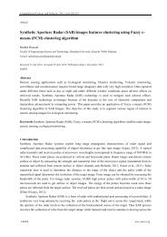
(5.2) Trigger regime (regime <strong>with</strong> two stable stationary states in phase space) was also observed. For example,<br />
this regime was realized for the following values <strong>of</strong> <strong>model</strong> parameters (Fig. 2): c 0. 1<br />
004 , c 6 2 ,<br />
P<br />
0<br />
120 , <br />
p<br />
2 , 0 x<br />
10 , 1 x<br />
5 , <br />
x<br />
0. 2 , 0 y<br />
0. 1 , <br />
p<br />
0. 0009 , 60 , 1 y<br />
7 ,<br />
<br />
x<br />
[0,3] . For every fixed value <strong>of</strong> <br />
x<br />
amount <strong>of</strong> parameter <br />
y<br />
was calculated <strong>with</strong> following formula:<br />
<br />
x 0<br />
<br />
y<br />
<br />
x<br />
( 0.0001)<br />
0 y<br />
. (8)<br />
<br />
x<br />
Fig. 2 Changing <strong>of</strong> stationary levels P <strong>of</strong> variable P (t)<br />
at increase <strong>of</strong> coefficient <strong>of</strong> <strong>interaction</strong> between sick and healthy<br />
individuals <br />
x<br />
and <br />
y<br />
determined by the equation (8) (blue and green lines). Red and black lines are determined by the<br />
equation (7).<br />
IAEES<br />
www.iaees.org
216<br />
Computational Ecology and S<strong>of</strong>tware, 2011, 1(4):208-217<br />
First point which corresponds to green line (black line corresponds to this point and determines by equation<br />
(7)) belongs to coordinate plane y 0 . The second point which corresponds to blue line (red line corresponds<br />
to this point and also determines by equation (7)) belongs to the domain 0 . It is obvious, that there exists<br />
a saddle point and surface <strong>of</strong> saddle’s incoming separatrixes separate domains <strong>of</strong> attractiveness <strong>of</strong> these two<br />
stable states. It is important to point out that such kind <strong>of</strong> <strong>dynamic</strong> regimes can be observed in nature for some<br />
species <strong>of</strong> forest <strong>insect</strong>s (Isaev et al., 1984, 2001, 2009). In particular, this <strong>dynamic</strong> regime can be realized in<br />
boreal forest zone for Xylotrechus altaicus Gebl. (Rozhkov, 1982; Vorontsov, 1978). Analysis which was<br />
provided by I.V. Ermolaev and presented in his publications (Ermolaev, 2011a, 2011b), showed that respective<br />
<strong>dynamic</strong> regime is realized for Protocryptis sibiricella Falk.<br />
4 Conclusion<br />
Analysis <strong>of</strong> three-component system which describes in simplest case the process <strong>of</strong> <strong>interaction</strong> between <strong>insect</strong><br />
<strong>population</strong> and <strong>food</strong> plant and pathogens, showed that even in the case when the speed <strong>of</strong> inflow <strong>of</strong> the <strong>food</strong><br />
into the system is constant and doesn’t depend on level <strong>of</strong> <strong>population</strong> size, we may have <strong>dynamic</strong> regimes <strong>with</strong><br />
several stationary states in phase space. Before (Isaev et al., 1984, 2001, 2009) this regime was called as fixed<br />
outbreak, and such kind <strong>of</strong> regimes can be observed in nature. Within the limits <strong>of</strong> two-component <strong>insect</strong> –<br />
<strong>food</strong> plant system such kind <strong>of</strong> <strong>dynamic</strong> regimes can also be observed (Nedorezov, 1986, 1997). But its<br />
realization depends on the reaction <strong>of</strong> <strong>food</strong> plant on <strong>population</strong> size increasing: it must have sufficient strong<br />
negative or positive feedback.<br />
Within the limits <strong>of</strong> the inset – pathogen system analogs <strong>of</strong> fixed outbreak can be realized too (Nedorezov,<br />
1986, 1997). But realization <strong>of</strong> this regime requires specific relations between components <strong>of</strong> the system. In<br />
considered <strong>model</strong> we had very simple assumptions about <strong>interaction</strong> between various components <strong>of</strong> the<br />
system. Nevertheless, simple assumptions can lead to realization <strong>of</strong> complicated <strong>dynamic</strong>al regimes.<br />
Acknowledgement<br />
This publication was supported by RFFI grant 11-04-01295-a.<br />
References<br />
Andronov AA, Vitt AA, Khaikin SE. 1959. Theory <strong>of</strong> Fluctuations. Fizmatgiz, Moscow, Russia (in Russian)<br />
Berryman AA. 1981. Population Systems: A General Introduction. Plenum Press, New York, USA<br />
Berryman AA. 1982. Biological control, thresholds and pest outbreaks. Environmental Entomology, 11(3):<br />
544-549<br />
Berryman AA, Stenseth NChr, Isaev AS. 1987. Natural regulation <strong>of</strong> herbivorous forest <strong>insect</strong> <strong>population</strong>s.<br />
Oecologia, 71: 174-184<br />
Ermolaev IV. 2011a. Behaviour <strong>of</strong> Protocryptis sibiricella Falk. in Natural Locations. Report 1. Zoological<br />
Journal, 90(2): 156-161<br />
Ermolaev IV. 2011b. Behaviour <strong>of</strong> Protocryptis sibiricella Falk. in Natural Locations. Report 2. Zoological<br />
Journal, 90(3): 325-330<br />
Isaev AS, Girs GI. 1975. Interaction between Trees and Xylophagous Insects. Nauka, Novosibirsk, Russia (in<br />
Russian)<br />
Isaev AS, Khlebopros RG, Nedorezov LV, et al. 1984. Population Dynamics <strong>of</strong> Forest Insects. Nauka,<br />
Novosibirsk, Russia (in Russian)<br />
Isaev AS, Khlebopros RG, Nedorezov LV, et al. 2001. Forest Insect Population Dynamics. Nauka, Moscow,<br />
Russia (in Russian)<br />
IAEES<br />
www.iaees.org
Computational Ecology and S<strong>of</strong>tware, 2011, 1(4):208-217<br />
217<br />
Isaev AS, Khlebopros RG, Nedorezov LV, et al. 2009. Forest Insect Population Dynamics. KMK, Novosibirsk,<br />
Russia<br />
Kolmogor<strong>of</strong>f AN. 1937. Sulla theoria di Volterra della lutta per l'esistenza. Giornale dell'Inst Italiano degli<br />
attuary, 7: 74-80<br />
Konikov AS. 1978. Regulators <strong>of</strong> Forest Insect Populations. Nauka, Novosibirsk, Russia (in Russian).<br />
Nedorezov LV. 1986. Modeling <strong>of</strong> Forest Insect Outbreaks. Nauka, Novosibirsk, Russia (in Russian)<br />
Nedorezov LV. 1997. Escape-effect and <strong>population</strong> outbreaks. Ecological Modelling, 94: 95-110<br />
Nedorezov LV, Utyupin YuV. 2011. Continuous-Discrete Models <strong>of</strong> Population Dynamics. State Public<br />
Scientific-Technical Library <strong>of</strong> the Siberian Branch <strong>of</strong> Russian Academy <strong>of</strong> Sciences, Novosibirsk, Russia<br />
(in Russian)<br />
Nedorezov LV. 2011. Analysis <strong>of</strong> some experimental time series by Gause: application <strong>of</strong> simple mathematical<br />
<strong>model</strong>s. Computational Ecology and S<strong>of</strong>tware, 1(1): 25-36<br />
Rozhkov AS. 1982. Tree and Insect. Nauka, Novosibirsk, Russia (in Russian)<br />
Smith JM. 1974. Models in Ecology. Cambridge University Press, Cambridge, UK<br />
Varley GC, Gradwell GR, Hassell MP. 1973. Insect Population Ecology: an Analytical Approach. Blackwell<br />
Scientific, Oxford, UK<br />
Volterra V. 1931. Lecons sur la theorie mathematique de la lutte pour la vie. Gauthiers-Villars, Paris, France<br />
Vorontsov AI. 1963. Basic Biology for Forest Protection. Visshaya Shkola, Moscow, Russia (in Russian)<br />
Vorontsov AI. 1978. Forest Pathology. Forest Industry, Moscow, Russia (in Russian)<br />
IAEES<br />
www.iaees.org