Basis Reduction and the Complexity of Branch-and-Bound 1 ...

Basis Reduction and the Complexity of
Branch-and-Bound
Gábor Pataki ∗ Mustafa Tural † Erick B. Wong ‡§
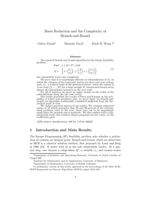
Abstract
The classical branch-and-bound algorithm for the integer feasibility
problem
Find
Q =
¯x ∈ Q ∩ Z n , with
{ ( )
l1
x | ≤
l 2
( A
I
)
x ≤
(
w1
w 2
)}
has exponential worst case complexity.
We prove that it is surprisingly efficient on reformulations of (1), in
which the columns of the constraint matrix are short and near orthogonal,
i.e., a reduced basis of the generated lattice: when the entries of
A are from {1, . . ., M} for a large enough M, branch-and-bound solves
almost all reformulated instances at the root node.
For all A matrices we prove an upper bound on the width of the
reformulations along the last unit vector.
Our results generalize the results of Furst and Kannan on the solvability
of subset sum problems; also, we prove them via branch-andbound,
an algorithm traditionally considered inefficient from the theoretical
point of view.
We explore practical aspects of our results. We compute numerical
values of M which guarantee that 90 and 99 percent of the reformulated
problems solve at the root: these turn out to be surprisingly
small when the problem size is moderate. We also confirm with a computational
study that random integer programs become easier, as the
coefficients grow.
AMS subject classifications: 90C10, 11Y16, 68Q25
(1)
1 Introduction and Main Results
The Integer Programming (IP) feasibility problem asks whether a polyhedron
Q contains an integral point. Branch-and-bound, which we abbreviate
as B&B is a classical solution method, first proposed by Land and Doig
in 1960 [24]. It starts with Q as the sole subproblem (node). In a general
step, one chooses a subproblem Q ′ , a variable x i , and creates nodes
∗ Department of Statistics and Operations Research, University of North Carolina at
Chapel Hill
† Institute for Mathematics and its Applications, University of Minnesota
‡ Department of Mathematics, University of British Columbia
§ A preliminary version of this article appeared in the proceedings of the 2010 ACM-
SIAM Symposium on Discrete Algorithms (SODA), pages 1254-1261
1

Q ′ ∩ {x|x i = γ}, where γ ranges over all possible integer values of x i . We repeat
this until all subproblems are shown to be empty, or we find an integral
point in one of them.
x 2
13
12
11
10
9
8
7
6
5
4
3
y 2
18
17
16
15
14
13
12
11
10
9
8
2
1
0
0 1 2 3 4 5 6 7 8 9 10 11 12 13
x 1
7
6
5
−244 −242 −240 −238 −236 −234 −232 −230 −228
y 1
Figure 1: The polyhedron of Example 1 before and after the reformulation
B&B (and its version used to solve optimization problems) enhanced by
cutting planes is a dependable algorithm implemented in most commercial
software packages. However, instances in [16, 9, 15, 21, 3, 4] show that it
is theoretically inefficient: it may take an exponential number of subproblems
to prove the infeasibility of simple knapsack problems. While B&B
is inefficient in the worst case, Cornuéjols et al. in [11] developed useful
computational tools to give an early estimate on the size of the B&B tree
in practice.
Since IP feasibility is NP-complete, one can ask for polynomiality of a
solution method only in fixed dimension. All algorithms that achieve such
complexity rely on advanced techniques. The algorithms of Lenstra [26]
and Kannan [19] first round the polyhedron (i.e., apply a transformation to
make it have a spherical appearance), then use basis reduction to reduce the
problem to a provably small number of smaller dimensional subproblems.
On the subproblems the algorithms are applied recursively, e.g., rounding
is done again. Generalized basis reduction, proposed by Lovász and Scarf
in [27] avoids rounding, but needs to solve a sequence of linear programs to
create the subproblems. For surveys on the connection of basis reduction,
and integer programming we refer to Kannan [18] and Eisenbrand [12].
There is a simpler way to use basis reduction in integer programming:
preprocessing (1) to create an instance with short and near orthogonal
columns in the constraint matrix, then simply feeding it to an IP solver.
2

The first such reformulation method, that we call nullspace reformulation,
was proposed by Aardal, Hurkens and Lenstra for equality constrained integer
programs in [2], and further studied in [1]. The rangespace reformulation
of Krishnamoorthy and Pataki [21] applies to general integer programs. We
describe these below, assuming that A is an integral matrix with m rows
and n columns, and the w i and l i are integral vectors.
The rangespace reformulation of (1) is
Find ȳ ∈ Q R ∩ Z n , with
{ ( )
l1
Q R = y | ≤
l 2
( A
I
)
Uy ≤
(
w1
w 2
)}
,
where U is a unimodular matrix computed to make the columns of the
constraint matrix a reduced basis of the generated lattice.
The nullspace reformulation is applicable when w 1 = l 1 . Assuming that
the rows of A are linearly independent, it is
Find ȳ ∈ Q N ∩ Z n−m , with
Q N = {y |l 2 − x 0 ≤ By ≤ w 2 − x 0 } ,
where x 0 ∈ Z n satisfies Ax 0 = l 1 , and the columns of B are a reduced basis
of the lattice {x ∈ Z n |Ax = 0 }.
We analyze the use of Lenstra-Lenstra-Lovász (LLL) [25], and reciprocal
Korkin-Zolotarev (RKZ) reduced bases [22] in the reformulations, and use
Korkin-Zolotarev (KZ) reduced bases [19, 20] in our computational study.
We will review the relevant properties of these bases in Section 2.
When Q R is computed using LLL reduction, we call it the LLL-rangespace
reformulation of Q, and abusing notation we also call (2) the LLL-rangespace
reformulation of (1). Similarly we talk about LLL-nullspace, RKZ-rangespace,
and RKZ-nullspace reformulations.
Example 1. The polyhedron
672 ≤ 61x 1 + 59x 2 ≤ 707
0 ≤ x 1 ,x 2 ≤ 12
is shown on the first picture of Figure 1. It is long and thin, and defines
an infeasible and relatively difficult integer feasibility problem for B&B, as
branching on either x 1 or x 2 yields 12 subproblems. Lenstra’s and Kannan’s
algorithms would first transform this polyhedron to make it more spherical;
generalized basis reduction would solve a sequence of linear programs to find
the direction x 1 + x 2 along which the polyhedron is thin.
The LLL-rangespace reformulation is
672 ≤ −2x 1 + 19x 2 ≤ 707
0 ≤ −x 1 − 20x 2 ≤ 12
0 ≤ x 1 + 21x 2 ≤ 12
3
(2)
(3)
(4)
(5)

shown on the second picture of Figure 1: it is still long, and thin, but now
branching on y 2 proves integer infeasibility. (A similar example was given
in [21]).
The reformulation methods are easier to describe, than, say Lenstra’s
algorithm, and are also successful in practice in solving several classes of hard
integer programs: see [2, 1, 21]. For instance, the original formulations of
the marketshare problems of Cornuéjols and Dawande in [10] are notoriously
difficult for commercial solvers, while the nullspace reformulations are much
easier to solve as shown by Aardal et al. in [1].
However, they seem difficult to analyze in general. For an overview of
previous results, we need the following concepts: if Q is a polyhedron and z
is a nonzero integral vector, then the width, and integer width of Q along z
are
width(z,Q) = max {〈z,x〉} − min {〈z,x〉} , and
x∈Q x∈Q
⌊ ⌋ ⌈ ⌉
iwidth(z,Q) = max {〈z,x〉} − min {〈z,x〉} + 1.
x∈Q x∈Q
The quantity iwidth(z,Q) is the number of subproblems generated, when
branching on the hyperplane 〈z,x〉 in seeking to find an integral point in Q.
In particular, iwidth(z,Q) = 0 implies that Q has no integral point.
Krishnamoorthy and Pataki in [21] studied knapsack problems with a
constraint vector a having a given decomposition a = λp + r, with p and r
integral vectors, and λ an integer, large compared to ‖ p ‖ and ‖ r ‖. They
proved
width(e n ,Q R ) ≤ width(p,Q), (6)
iwidth(e n ,Q R ) ≤ iwidth(p,Q), (7)
and analogous results for the nullspace reformulation. (In fact, as shown in
[31], equality holds in (6) and (7).)
These inequalities partially explain why the reformulation techniques
are effective: considering (6), note that width(p,Q) is small, due to λ being
large, i.e., p being near parallel to the constraint vector. Also, for a
wide variety of problems iwidth(p,Q) = 0, but branching on the individual
variables would need an exponential number of B&B nodes: as (7) shows,
for these problems branching on the last variable in Q R proves infeasibility
at the root node. In other words, the effect of branching on 〈p,x〉 in Q is
mimicked by branching on a single variable in Q R .
In a general analysis, one could hope for proving polynomiality of B&B
on the reformulations of (1) when the dimension is fixed. This seems difficult.
However, we give a different and perhaps even more surprising complexity
analysis. It is in the spirit of Furst and Kannan’s work in [14] on subset
4

sum problems and builds on a generalization of their Lemma 1 to bound
the fraction of integral matrices for which the shortest nonzero vectors of
certain corresponding lattices are short. We also use an upper bound on
the size of the B&B tree, which depends on the norms of the Gram-Schmidt
vectors of the constraint matrix. We introduce necessary notation and state
our results, then give a comparison with [14].
When a statement is true for all, but at most a fraction of 1/2 n of the
elements of a set S, we say that it is true for almost all elements. The value
of n will be clear from the context. Reverse B&B is B&B branching on the
variables in reverse order starting with the one of highest index. We assume
w 2 > l 2 and for simplicity of stating the results we also assume n ≥ 5. For
positive integers m, n and M we denote by G m,n (M) the set of matrices with
m rows and n columns, and the entries drawn from {1,... ,M}. We denote
by G ′ m,n(M) the subset of G m,n (M) consisting of matrices with linearly
independent rows, and let
χ m,n (M) = |G′ m,n(M)|
|G m,n (M)| . (8)
In Lemma 4 in Section 2 we will prove a lower bound on χ m,n (M) for any
n,m and M using only elementary
(
techniques. For matrices (and vectors)
A
A and B, we write (A;B) for . For an m by n integral matrix A with
B)
independent rows we write gcd(A) for the greatest common divisor of the
m by m subdeterminants of A. If B&B generates at most one node at each
level of the tree, we say that it solves an integer feasibility problem at the
root node. If l 1 = w 1 , and the system Ax = l 1 does not have an integral
solution, then the nullspace reformulation cannot be constructed. In this
case we also say that B&B solves the nullspace reformulation at the root
node.
Given independent vectors b 1 ,...,b r , the vectors b ∗ 1 ,... ,b∗ r form the
Gram-Schmidt orthogonalization of b 1 ,...,b r , if b ∗ 1 = b 1, and b ∗ i is the
projection of b i onto the orthogonal complement of the subspace spanned
by b 1 ,...,b i−1 for i ≥ 2.
The main results of the paper follow.
Theorem 1. The following hold.
(1) If M ≥ (2n ‖(w 1 ;w 2 ) − (l 1 ;l 2 )‖) n/m+1 , then for almost all A ∈ G m,n (M)
reverse B&B solves the RKZ-rangespace reformulation of (1) at the
root node.
(2) If M ≥ (12(n − m) ‖w 2 − l 2 ‖) n/m , then for almost all A ∈ G ′ m,n (M)
reverse B&B solves the RKZ-nullspace reformulation of (1) at the root
node.
5

The proofs also show that when M obeys the above bounds, then Q∩Z n
has at most one element for almost all A ∈ G m,n (M) (or almost all A ∈
G ′ m,n (M)). Note that when n/m is fixed and the problems are binary, and
equality constrained, the magnitude of M required is a polynomial in n.
Theorem 2. The conclusions of Theorem 1 hold for the LLL-reformulations,
if the bounds on M are
(2 (n+4)/2 ‖(w 1 ;w 2 ) − (l 1 ;l 2 )‖) n/m+1 ,
and
respectively.
(2 (n−m+4)/2 ‖w 2 − l 2 ‖) n/m ,
Furst and Kannan in [14] based on Lagarias’ and Odlyzko’s [23] and
Frieze’s [13] work show that the subset sum problem is solvable in polynomial
time using a simple iterative method for almost all weight vectors in G 1,n (M)
and all right hand sides, when M is sufficiently large and a reduced basis of
the orthogonal lattice of the weight vector is available. Their bound on M
is
M ≥ 2 (3/2)n log n+5n , (9)
when the basis is RKZ reduced, and
M ≥ 2 n2 /2+2n n 3n/2 , (10)
when it is LLL reduced.
Our bounds obtained by letting m = 1 in Theorems 1 and 2 are comparable,
when the size of M, i.e., ⌈log(M + 1)⌉ is concerned. With RKZ
reduction, both the bounds in Theorem 1 and the one in (9) require the size
of M to be O(n log n). With LLL reduction, our bounds in Theorem 2 and
the one in (10) require the size of M to be O(n 2 ). Hence, our results generalize
the solvability results of [14] from subset sum problems to bounded
integer programs; also, we prove them via branch-and-bound, an algorithm
considered inefficient from the theoretical point of view.
Solving almost all instances of a problem in polynomial time may not,
in general, lead to an algorithm with polynomial expected running time: for
a discussion, we refer to David S. Johnson’s survey [17]. However, we can
combine branch-and-bound on the original and reformulated problems to
obtain a composite algorithm, which does have polynomial expected running
time.
COMPOSITE ALGORITHM
6

(a) Compute the LLL-rangespace reformulation of (1), and let b ∗ i (i =
1,... ,n) be the Gram-Schmidt orthogonalization of the constraint matrix.
Check whether ‖b ∗ i ‖>‖(w 1;w 2 ) − (l 1 ;l 2 )‖, for all i = 1,... ,n,
(b) If the answer is YES, run reverse B&B on the reformulated problem,
and STOP.
(c) Otherwise, run B&B on the original problem, choosing the branching
variables in an arbitrary sequence.
Theorem 3. Let B := ∏ n
i=1 (⌊(w 2,i − l 2,i )⌋ + 1), and assume
M ≥ B 1/m (2 (n+1)/2 ‖(w 1 ;w 2 ) − (l 1 ;l 2 )‖ +2) (n+m)/m .
Then the Composite Algorithm runs in expected polynomial time, if A is
uniformly and independently chosen from G m,n (M).
Remark 1. It is easy to check that Theorems 1 through 3 remain true, if
the set {1,... ,M} is replaced by an arbitrary set of M distinct integers.
Smoothed complexity [34, 35] is a more recent notion that successfully
explains why some algorithms with an exponential worst case running time
are usually much faster. Beier and Vöcking in [5] presented smoothed complexity
results for binary integer programs, and generalizing these, Röglin
and Vöcking in [32] characterized the smoothed complexity of general integer
programs in terms of their worst case complexity. Their results imply
polynomial smoothed complexity of packing and covering integer programs
with a fixed number of constraints. Our assumptions and results are quite
different, and most importantly, the tool we use is the classical branch-andbound
algorithm.
Proposition 1 gives another indication why the reformulations are relatively
easy. One can observe that det(AA T ) can be quite large even for
moderate values of M, if A ∈ G m,n (M) is a random matrix with m ≤ n.
For instance, for a random A ∈ G 4,30 (100) we found det(AA T ) to be of the
order 10 18 . We can bound the width of the reformulations along the last
unit vector for any A (i.e., not just almost all).
Proposition 1. If Q R is computed using RKZ reduction, then
width(e n ,Q R ) ≤
√ n ‖(w1 ;w 2 ) − (l 1 ;l 2 )‖
det(AA T + I) 1/(2n) . (11)
Also, if A has independent rows, and Q N is computed using RKZ reduction,
then
width(e n−m ,Q N ) ≤ gcd(A)√ n − m ‖w 2 − l 2 ‖
det(AA T ) 1/(2(n−m)) . (12)
7

The same results hold for the LLL-reformulations, if √ n and √ n − m are
replaced by 2 (n−1)/4 and 2 (n−m−1)/4 , respectively.
Remark 2. As described in [30] for the nullspace reformulation, and in Section
5 of [21] for both reformulations, directions achieving the same widths
exist in Q, and they can be quickly computed from the U matrix in (2),
or the B matrix in (3). For instance, if p is the last row of U −1 , then
width(e n ,Q R ) = width(p,Q) and iwidth(e n ,Q R ) = iwidth(p,Q).
A practitioner of integer programming may ask for the value of Theorems
1 and 2. Proposition 2 and a computational study put these results into a
more practical perspective. Proposition 2 shows that when m and n are not
too large, already fairly small values of M guarantee that the RKZ-nullspace
reformulation (which has the smallest bound on M) of the majority of binary
integer programs get solved at the root node.
Proposition 2. Suppose that m and n are chosen according to Table 1, and
M is as shown in the third column. Then for at least 90% of A ∈ G ′ m,n(M)
n m M for 90 % M for 99 %
20 10 99 124
30 20 31 35
40 30 21 23
50 40 18 19
30 10 3478 4378
40 20 229 256
50 30 93 100
40 10 169000 212758
50 20 1844 2069
60 30 410 442
70 40 193 205
Table 1: Values of M to make sure that the RKZ-nullspace reformulation
of 90 or 99% of the instances of type (13) solve at the root node
and all b right hand sides, reverse B&B solves the RKZ-nullspace reformulation
of
Ax = b
x ∈ {0,1} n (13)
at the root node. The same is true for 99% of A ∈ G ′ m,n (M), if M is as
shown in the fourth column.
8

M
EQUALITY
INEQUALITY
Feas/Infeas Nodes: before/after Feas/Infeas Nodes: before/after
100 1/14 1,020,790/979 14/1 417,304/1,754
1000 0/15 1,104,037/89 0/15 1,197,996/905
10000 0/15 1,097,806/23 0/15 1,137,544/111
Table 2: Computational results with m = 4 and n = 30.
M
EQUALITY
INEQUALITY
Feas/Infeas Nodes: before/after Feas/Infeas Nodes: before/after
100 7/8 94,311,230/17,340 15/0 9,422,016/48,321
1000 0/15 154,552,544/2,202 0/15 ∗ ∗ ∗/25,342
10000 0/15 173,085,573/178 0/15 ∗ ∗ ∗/2,806
Table 3: Computational results with m = 5 and n = 40.
Note that 2 n−m is the best upper bound one can give on the number
of nodes when B&B is run on the original formulation (13); also, randomly
generated IPs with n − m = 30 are nontrivial even for commercial solvers.
According to Theorems 1 and 2, random integer programs with coefficients
drawn from {1,... ,M } should get easier, as M grows. Our computational
study confirms this somewhat counterintuitive hypothesis on the
family of marketshare problems of Cornuéjols and Dawande in [10].
We generated fifteen 4 by 30, fifteen 5 by 40 and fifteen 6 by 50 matrices
with entries drawn from {1,... ,M} with M = 100,1000 and 10000 (this is
135 matrices overall), set b = ⌊Ae/2⌋, where e is the vector of all ones, and
constructed the instances of type (13), and
b − e ≤ Ax ≤ b
x ∈ {0,1} n .
(14)
The latter of these are a relaxed version, which correspond to trying to
find an almost-equal market split.
Since RKZ reduction is not implemented in any software that we know of,
we used the Korkin-Zolotarev (KZ) reduction routine from the NTL library
[33] to compute the reformulations.
Tables 2, 3 and 4 summarize our computational study. The column
“Feas/Infeas” shows the number of feasible vs. infeasible instances: this is
relevant, since the latter tend to be more difficult. The column “Nodes:
before/after” shows the average number of nodes (rounded to the nearest
9

M
EQUALITY
INEQUALITY
Feas/Infeas Nodes: before/after Feas/Infeas Nodes: before/after
100 9/6 ∗ ∗ ∗/890,235 15/0 ∗ ∗ ∗/2,108,615
1000 0/15 ∗ ∗ ∗/43,446 0/15 ∗ ∗ ∗/1,975,226
10000 0/15 ∗ ∗ ∗/3,237 0/15 ∗ ∗ ∗/77,018
Table 4: Computational results with m = 6 and n = 50.
integer) that the commercial IP solver CPLEX 11.0.1 took to solve the original
formulation, the rangespace reformulation of the inequality-constrained
and the nullspace reformulation of the equality-constrained problems. The
entry “***” means that the computation did not finish after 3 hours of computing
time on an Intel Core 2 Duo 2.26 GHz laptop with 1.98 GB of RAM.
(More precisely, two out of fifteen 5 × 40 inequality constrained instances
with M = 1000 finished, and four out of fifteen 6×50 inequality constrained
instances with M = 100 finished. Among the others, none finished within
the allotted time limit.)
The original problems do not become easier with larger M. For the reformulated
instances the reduction in the number of nodes is less pronounced,
but still significant, when a larger M results in more infeasible instances.
Overall, the tables confirm the theoretical findings of the paper: reformulations
of random integer programs become easier as the size of the coefficients
grows.
In Section 2 we introduce further notation and prove our main results.
2 Further Notation and Proofs
A lattice is a set of the form
L = L(B) = { Bx |x ∈ Z r } , (15)
where B is a real matrix with r independent columns, called a basis of L
and r is called the rank of L.
The Euclidean norm of a shortest nonzero vector in L is denoted by
λ 1 (L), and Hermite’s constant is
{
λ1 (L) 2
}
C j = sup
(det L) 2/j |Lis a lattice of rank j . (16)
Here detL is the determinant of the lattice, defined as
√
det L = detB T B, (17)
with detL actually independent of the choice of the basis B.
10

We define
γ i = max { C 1 ,... ,C i } . (18)
A matrix A defines two lattices that we are interested in:
L R (A) = L(A;I), L N (A) = {x ∈ Z n |Ax = 0} , (19)
where we recall that (A;I) is the matrix obtained by stacking A on top of
I.
We do not define LLL and RKZ reducedness formally, only collect their
properties that we will use below:
Lemma 1. Suppose that b 1 ,...,b r is a basis of the lattice L with Gram-
Schmidt orthogonalization b ∗ 1 ,... ,b∗ r and i ∈ {1,... ,r}. Then
(1) if b 1 ,... ,b r is RKZ reduced, then
‖b ∗ i ‖≥ λ 1(L)/C i , (20)
and
‖b ∗ r ‖≥ (det L)1/r / √ r. (21)
(2) if b 1 ,... ,b r is LLL reduced, then
‖b ∗ i ‖≥ λ 1 (L)/2 (i−1)/2 , (22)
and
‖b ∗ r ‖≥ (detL)1/r /2 (r−1)/4 . (23)
Proof Statements (20) and (21) are proven in [22], and (22) is shown in
[25]. We now consider the inequalities
‖b ∗ i ‖≤ 2(r−i)/2 ‖b ∗ r ‖ (i = 1,... ,r), (24)
which hold when the basis is LLL reduced. Multiplying them and using
‖b ∗ 1 ‖ ... ‖b∗ r ‖= detL gives (23).
Lemma 2. Let P be a polyhedron
P = {y ∈ R r |l ≤ By ≤ w} , (25)
and b ∗ 1 ,...,b∗ r the Gram-Schmidt orthogonalization of the columns of B.
When reverse B&B is applied to P, the number of nodes on the level of
y i is at most
(⌊ ⌋ ) (⌊ ⌋ )
‖w − l‖
‖w − l‖
‖b ∗ i ‖ + 1 ...
‖b ∗ + 1 . (26)
r ‖
11

Proof First we show
width(e r ,P) ≤ ‖w − l‖ / ‖b ∗ r ‖ . (27)
Let y r,1 and y r,2 denote the maximum and the minimum of y r over P. Writing
¯B for the matrix composed of the first r −1 columns of B and b r for the
last column, it holds that there is y 1 ,y 2 ∈ R r−1 such that ¯By 1 + b r y r,1 and
¯By 2 + b r y r,2 are in P. So
‖w − l‖ ≥ ‖( ¯By 1 + b r y r,1 ) − ( ¯By 2 + b r y r,2 )‖
= ‖ ¯B(y 1 − y 2 ) + b r (y r,1 − y r,2 )‖
≥ ‖b ∗ r ‖ |y r,1 − y r,2 |
= ‖b ∗ r ‖ width(e r ,P)
holds, and so does (27).
After branching on y r ,...,y i+1 , each subproblem is defined by a matrix
formed of the first i columns of B, and bound vectors, which are translates
of l and w by the same vector. Hence the above proof implies that the width
along e i in each of these subproblems is at most
‖w − l‖ / ‖b ∗ i ‖, (28)
and this completes the proof.
Our Lemma 3 builds on Furst and Kannan’s Lemma 1 in [14], with part
(2) also being a direct generalization.
Lemma 3. Let r > 0. Then
(1) the fraction of A ∈ G m,n (M) with λ 1 (L R (A)) ≤ r is at most
(2⌊r⌋ + 1) n+m
M m .
(2) the fraction of A ∈ G ′ m,n (M) with λ 1(L N (A)) ≤ r is at most
(2⌊r⌋ + 1) n
M m χ m,n (M) .
Proof We first prove (2). For v, a fixed nonzero vector in Z n , consider
the equation
Av = 0. (29)
There are at most M m(n−1) matrices in G ′ m,n (M) that satisfy (29): if the
components of n − 1 columns of A are fixed, then the components of the
column corresponding to a nonzero entry of v are determined from (29).
12

The number of vectors in Z n with norm at most r is at most (2⌊r⌋+1) n :
if v ∈ Z n satisfies ‖v ‖≤ r, then |v i | ≤ r for all i, hence |v i | ≤ ⌊r⌋ for all i.
Also, the number of matrices in G ′ m,n(M) is M mn χ m,n (M). Therefore the
sought ratio is bounded by
(2⌊r⌋ + 1) n M m(n−1)
M mn χ m,n (M)
=
(2⌊r⌋ + 1)n
M m χ m,n (M) .
For (1), note that (v 1 ;v 2 ) ∈ Z m+n is a nonzero vector in L R (A), iff v 2 ≠ 0
and
Av 2 = v 1 . (30)
An argument like the one in the proof of (2) shows that for fixed (v 1 ;v 2 ) ∈
Z m+n with v 2 ≠ 0, there are at most M m(n−1) matrices in G m,n (M) that
satisfy (30).
The number of vectors in Z n+m with norm at most r is at most (2⌊r⌋ +
1) n+m , and the number of matrices in G m,n (M) is M mn . Hence the ratio
we are interested in is bounded by
(2⌊r⌋ + 1) n+m M m(n−1)
M mn
=
(2⌊r⌋ + 1)n+m
M m .
Let us recall the definition of χ m,n (M) from (8). *** Martin and Wong in
[28] showed that χ m,m (M) (and therefore also χ m,n (M) for m ≤ n) is of the
order 1 −o(1), as M → ∞; Bourgain et al. in [7] prove χ m,m (M) = 1 −o(1),
as m → ∞.
In Theorems 1 and 2 we use χ m,n (M) ≥ 1/2 for simplicity. In the proof
of Proposition 2, however, we need a stronger statement, which we prove in
Lemma 4 below. We remark, that the results of [28] and [7] are asymptotic,
whereas Lemma 4 does not use any constants, and holds for any m,n, and
M.
Lemma 4. For positive integers m, n, and M with m ≤ n,
χ m,n (M) ≥ 1 −
1
(M − 1)Mn−m. (31)
Proof We use ideas from the solution to problem B4 in the 67 th William
Lowell Putnam Mathematical Competition. We first need the following:
Claim Let V ⊆ R n be an affine subspace of dimension k. Then
|V ∩ {1,... ,M} n | ≤ M k . (32)
Proof of Claim We use induction on k+n. The statement is clearly true,
when k +n ≤ 1, and also when n is arbitrary, and k = 0. Now, suppose that
V ⊆ R n is an affine subspace of dimension k. Let
V i = V ∩ {x|x n = i }(i = 1,... ,M).
13

Case 1 If V i is at most k−1 dimensional for all i, then these sets have an intersection
of cardinality at most M k−1 with {1,... ,M} n by the induction
hypothesis. Therefore,
|V ∩ {1,... ,M} n | ≤
M∑
M k−1 = M k .
i=1
Case 2 If V i is k dimensional for some i, then V = V i , i.e., all the vectors in V
have i in the last coordinate. Now let V ′ ⊆ R n−1 be the k dimensional
affine subspace obtained from V by dropping the last coordinate. We
have
|V ∩ {1,... ,M} n | = |V ′ ∩ {1,... ,M} n−1 | ≤ M k ,
where the last inequality again follows from the induction hypothesis.
End of Proof of Claim
Now, let A be an m by n random matrix with coefficients chosen uniformly
and independently from {1,... ,M}. For 2 ≤ i ≤ m, let D i be the event that
the ith row of A is a linear combination of the first i −1 rows. By the Claim
there are at most M i−1 vectors in the subspace spanned by the first i − 1
rows which have components in {1,... ,M}. So
holds. Therefore,
P(D i ) ≤ M i−1 /M n .
P(A has dependent rows ) ≤
≤
∑ m
i=2 P(D i) ≤ ∑ m
1
(M − 1)(M n−m ) ,
i=2 Mi−1 /M n
and this completes the proof.
Proof of Theorems 1 and 2 For part (1) in Theorem 1, let b ∗ 1 ,...,b∗ n be
the Gram-Schmidt orthogonalization of the columns of (A;I)U. Lemma 2
implies that reverse B&B solves (2) at the root, if
‖b ∗ i ‖>‖(w 1 ;w 2 ) − (l 1 ;l 2 )‖ (33)
for i = 1,... ,n. Let us now recall the definition of C i from (16), and of
γ i from (18). Since the columns of (A;I)U form an RKZ reduced basis of
L R (A), (20) implies
‖b ∗ i ‖≥ λ 1 (L R (A))/C i . (34)
So (33) holds, when
λ 1 (L R (A)) > C i ‖(w 1 ;w 2 ) − (l 1 ;l 2 )‖ (35)
14

does for i = 1,... ,n, which is in turn implied by
λ 1 (L R (A)) > γ n ‖(w 1 ;w 2 ) − (l 1 ;l 2 )‖ . (36)
Let ɛ be a real number between 0 and 1. By Lemma 3, the fraction of
A ∈ G m,n (M) matrices for which (36) does not hold is at most ɛ, when
i.e., when
(2⌊γ n ‖(w 1 ;w 2 ) − (l 1 ;l 2 )‖⌋ + 1) n+m
M m ≤ ɛ,
M ≥ (2⌊γ n ‖(w 1 ;w 2 ) − (l 1 ;l 2 )‖⌋ + 1) (n+m)/m
ɛ 1/m . (37)
Using the known estimate γ n ≤ 1 + n/4 (see for instance [29]) , setting
ɛ = 1/2 n , and doing some algebra with (37) yields the required result.
The proof of part (2) of Theorem 1 is along the same lines: now b ∗ 1 ,...,b∗ n−m
is the Gram-Schmidt orthogonalization of the columns of B, which is an RKZ
reduced basis of L N (A). Lemma 2 and the reducedness of B implies that
reverse B&B solves (3) at the root, if
λ 1 (L N (A)) > γ n−m ‖w 2 − l 2 ‖ . (38)
Again, letting ɛ be a real number between 0 and 1, Lemma 3 implies that
the fraction of matrices in G ′ m,n(M) which do not satisfy (38) is at most ɛ,
if
(2⌊γ n−m ‖w 2 − l 2 ‖⌋ + 1) n
M m ≤ ɛ,
χ m,n (M)
that is, when
M ≥ (⌊2γ n−m ‖w 2 − l 2 ‖⌋ + 1) n/m
ɛ 1/m (χ m,n (M)) 1/m . (39)
Then simple algebra and using χ m,n (M) ≥ 1/2 completes the proof.
The proof of Theorem 2 is an almost verbatim copy, now using the estimate
(22) to lower bound ‖b ∗ i ‖.
Remark 3. Theorems 1 and 2 rely on inequalities (20) and (22), respectively.
If b 1 ,...,b r is a KZ reduced basis of the lattice L, then
‖b ∗ i ‖≥ λ 1 (L)/i (1+log i)/2 , (40)
(see [22]), so results of intermediate strength can be shown when the reformulations
are computed using KZ reduction.
Proof of Theorem 3 When we end up in step (b), reverse branch-andbound
solves the LLL-reformulation of (1) at the root node. An argument
15

analogous to the one used in the proof of Theorem 2 implies that this happens
with probability at least 1 − 1/B, hence the expected number of nodes
that the Composite Algorithm looks at is at most
(
n 1 − 1 )
+ B 1 B B ≤ n + 1.
Since a node can be processed in time polynomial in the size of the instance,
and the LLL-reformulation is computable in polynomial time, our claim
follows.
Proof of Proposition 1 Let b ∗ 1 ,... ,b∗ n be the Gram-Schmidt orthogonalization
of the columns of (A;I)U. Using (27) in the proof of Lemma 2
gives
Next, from (21) we obtain
width(e n ,Q R ) ≤ ‖(w 1;w 2 ) − (l 1 ;l 2 )‖
‖b ∗ . (41)
n ‖
‖b ∗ n ‖ ≥ (det L R(A)) 1/n
√ n
. (42)
Also, the definition of L R (A) implies
detL R (A) = det(AA T + I) 1/2 , (43)
and combining these three inequalities proves (11).
The proof of (12) is analogous, but now we need to use
det L N (A) = det(AA T ) 1/2 /gcd(A), (44)
whose proof can be found in [8] for instance. To prove the claims about the
LLL-reformulations, we need to use (23) (in place of (21)) to lower bound
‖b ∗ n ‖ or ‖b ∗ n−m ‖.
Proof of Proposition 2 Let N(n,r) denote the number of integral
points in the n-dimensional ball of radius r. In the previous proofs we
used (2⌊r⌋ + 1) n as an upper bound for N(n,r). The proof of Part (2) of
Theorem 1 actually implies that when
M ≥ (N(n,γ n−m ‖w 2 − l 2 ‖) 1/m
ɛ 1/m (χ m,n (M)) 1/m , (45)
then for all, but at most a fraction of ɛ of A ∈ G ′ m,n(M) reverse B&B solves
the RKZ-nullspace reformulation of (13) at the root node.
16

With ‖ w 2 − l 2 ‖= √ n we would like to compute the smallest M that
satisfies (45) for small values of n and m. First, let us consider Blichfeldt’s
upper bound [6]
C i ≤ 2 ( ) i + 4 2/i
π Γ . (46)
2
We verified computationally that the right hand side of (46) is an increasing
function of i, if i ≤ 30 (we are not aware of any analytical proofs). So
C n−m ≤ 2 ( ) n − m + 4 2/(n−m)
π Γ (47)
2
if n − m ≤ 30. Plugging (47) and (31) into (45) gives a valid lower bound
for M. We use the values ɛ = 0.1 and ɛ = 0.01 and dynamic programming
to exactly find the values of N(n,r), to obtain Table 1.
We note that in general N(n,r) is hard to compute, or find good upper
bounds for; however for small values of n and r a simple dynamic programming
algorithm finds the exact value quickly.
Acknowledgement We thank Van Vu for pointing out reference [7]. We are
very grateful to Greg Martin for discussions leading to the proof of Lemma
4.
References
[1] Karen Aardal, Robert E. Bixby, Cor A. J. Hurkens, Arjen K. Lenstra,
and Job W. Smeltink. Market split and basis reduction: Towards a
solution of the Cornuéjols-Dawande instances. INFORMS Journal on
Computing, 12(3):192–202, 2000.
[2] Karen Aardal, Cor A. J. Hurkens, and Arjen K. Lenstra. Solving a
system of linear Diophantine equations with lower and upper bounds
on the variables. Mathematics of Operations Research, 25(3):427–442,
2000.
[3] Karen Aardal and Arjen K. Lenstra. Hard equality constrained integer
knapsacks. Mathematics of Operations Research, 29(3):724–738, 2004.
[4] Karen Aardal and Arjen K. Lenstra. Erratum to: Hard equality
constrained integer knapsacks. Mathematics of Operations Research,
31(4):846, 2006.
[5] Rene Beier and Berthold Vöcking. Typical properties of winners
and losers in discrete optimization. SIAM Journal on Computing,
35(4):855–881, 2006.
17

[6] Hans Frederik Blichfeldt. A new principle in the geometry of numbers,
with some applications. Transactions of the American Mathematical
Society, 15(3):227–235, 1914.
[7] Jean Bourgain, Van H. Vu, and Philip Matchett Wood. On the singularity
probability of discrete random matrices. Journal of Functional
Analysis, to appear.
[8] J. W. S. Cassels. An introduction to the geometry of numbers. Springer,
1997.
[9] Vašek Chvátal. Hard knapsack problems. Operations Research,
28(6):1402–1411, 1980.
[10] Gérard Cornuéjols and Milind Dawande. A class of hard small 0–1
programs. INFORMS Journal on Computing, 11(2):205–210, 1999.
[11] Gérard Cornuéjols, Miroslav Karamanov, and Yanjun Li. Early estimates
of the size of branch-and-bound trees. INFORMS Journal on
Computing, 18(1):86–96, 2006.
[12] Friedrich Eisenbrand. Integer programming and algorithmic geometry
of numbers. In M. Juenger, Th.M. Liebling, D. Naddef, G.L.
Nemhauser, W.R. Pulleyblank, G. Reinelt, G. Rinaldi, and L.A.
Wolsey, editors, 50 Years of Integer Programming. Springer, New York,
NY, 2010.
[13] Alan Frieze. On the Lagarias-Odlyzko algorithm for the subset sum
problem. SIAM Journal on Computing, 15:536–540, 1986.
[14] Merrick Furst and Ravi Kannan. Succinct certificates for almost all
subset sum problems. SIAM Journal on Computing, 18:550 – 558,
1989.
[15] Zonghao Gu, George L. Nemhauser, and Martin W. P. Savelsbergh.
Lifted cover inequalities for 0–1 integer programs: Complexity. IN-
FORMS J. on Computing, 11:117–123, 1998.
[16] Robert G. Jeroslow. Trivial integer programs unsolvable by branchand-bound.
Mathematical Programming, 6:105–109, 1974.
[17] David S. Johnson. The NP-completeness column: An ongoing guide.
J. of Algorithms, 5:284–299, 1984.
[18] Ravi Kannan. Algorithmic geometry of numbers. Annual Review of
Computer Science, 2:231–267, 1987.
[19] Ravi Kannan. Minkowski’s convex body theorem and integer programming.
Mathematics of Operations Research, 12(3):415–440, 1987.
18

[20] A. Korkine and G. Zolotareff. Sur les formes quadratiques. Mathematische
Annalen, 6:366–389, 1873.
[21] Bala Krishnamoorthy and Gábor Pataki. Column basis reduction and
decomposable knapsack problems. Discrete Optimization, 6:242–270,
2009.
[22] Jeffrey C. Lagarias, Hendrik W. Lenstra, and Claus P. Schnorr. Korkin-
Zolotarev bases and successive minina of a lattice and its reciprocal
lattice. Combinatorica, 10(4):333–348, 1990.
[23] Jeffrey C. Lagarias and Andrew M. Odlyzko. Solving low-density subset
sum problems. Journal of ACM, 32:229–246, 1985.
[24] A. H. Land and Alison G. Doig. An automatic method for solving
discrete programming problems. Econometrica, 28:497–520, 1960.
[25] Arjen K. Lenstra, Hendrik W. Lenstra, Jr., and László Lovász. Factoring
polynomials with rational coefficients. Mathematische Annalen,
261:515–534, 1982.
[26] Hendrik W. Lenstra, Jr. Integer programming with a fixed number
of variables. First announcement (1979). Mathematics of Operations
Research, 8:538–548, 1983.
[27] László Lovász and Herbert E. Scarf. The generalized basis reduction
algorithm. Mathematics of Operations Research, 17:751–764, 1992.
[28] Greg Martin and Erick B. Wong. Almost all integer matrices have no
integer eigenvalues. The American Mathematical Monthly, 116:588–598,
2009.
[29] Jacques Martinet. Perfect Lattices in Euclidean Spaces. Springer-
Verlag, Berlin, 2003.
[30] Sanjay Mehrotra and Zhifeng Li. Branching on hyperplane methods
for mixed integer linear and convex programming using adjoint lattices.
Journal of Global Optimization, Online first, 2010.
[31] Gábor Pataki and Mustafa Tural. Basis reduction methods. In
James J. Cochran, Jr. Louis Anthony Cox, Pınar Keskinocak, Jeffrey P.
Kharoufeh, and J. Cole Smith, editors, To appear in Wiley Encyclopedia
of Operations Research and Management Science. John Wiley &
Sons, New York, NY, 2011.
[32] Heiko Röglin and Berthold Vöcking. Smoothed analysis of integer programming.
Mathematical Programming, 110(1):21–56, 2007.
19

[33] Victor Shoup. NTL: A Number Theory Library, 1990.
http://www.shoup.net.
[34] Daniel A. Spielman and Shang-Hua Teng. Smoothed analysis of algorithms
and heuristics: Progress and open questions. In Luis M. Pardo,
Allan Pinkus, Endre Süli, and Michael J. Todd, editors, Foundations
of Computational Mathematics, Santander 2005, volume 331 of London
Mathematical Society, Lecture Note Series, pages 274–342. Cambridge
University Press, Toronto, 2006.
[35] Daniel A. Spielman and Shang-Hua Teng. Smoothed analysis: an attempt
to explain the behavior of algorithms in practice. Communications
of the ACM, 52(10):76–84, 2009.
20