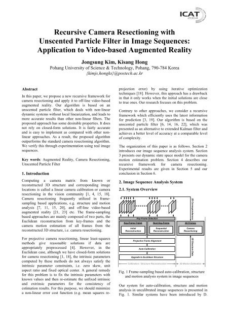
Recursive Camera Resectioning with Unscented Particle Filter in ...

Recursive Camera Resectioning with
Unscented Particle Filter in Image Sequences:
Application to Video-based Augmented Reality
Jongsung Kim, Kisang Hong
Pohang University of Science & Technology, Pohang, 790-784 Korea
{kimjs,hongks}@postech.ac.kr
Abstract
In this paper, we propose a new recursive framework for
camera resectioning and apply it to off-line video-based
augmented reality. Our algorithm is based on an
unscented particle filter, which deals with non-linear
dynamic systems without local linearization, and leads to
more accurate results than other non-linear filters. The
proposed approach has some desirable properties. It does
not rely on closed-form solutions. It is fairly accurate
and is easy to implement as compared with other nonlinear
approaches. As a result, the proposed algorithm
outperforms the standard camera resectioning algorithm.
We verify this through experimentation using real image
sequences.
Key words: Augmented Reality, Camera Resectioning,
Unscented Particle Filter
1. Introduction
Computing a camera matrix from known or
reconstructed 3D structure and corresponding image
locations is called a linear camera calibration or camera
resectioning in the vision community [1, 4, 15, 18].
Camera resectioning frequently utilized in framesampling
based applications, e.g. structure and motion
analysis [7, 11, 15, 20], and off-line video-based
augmented reality [21, 23] etc. The frame-sampling
based approaches are mainly composed of two parts, the
Euclidean reconstruction from key-frames and the
camera motion estimation of all frames from the
reconstructed 3D structure, i.e. camera resectioning.
For projective camera resectioning, linear least-squares
methods give reasonable solutions if data are
appropriately preprocessed [4]. However, in the
Euclidean case, although we have closed-form solutions
for camera resectioning [1, 18], the intrinsic parameters
computed by these methods do not always satisfy the
intrinsic parameter constraints, i.e. zero skew, unit
aspect ratio and fixed optical center. A general remedy
for this problem is to fix the intrinsic parameters with
known values and then re-estimate the unfixed intrinsic
and extrinsic parameters for the consistency of
estimation results. For this purpose, we should minimize
a non-linear error cost function (e.g. mean squares reprojection
error) by using iterative optimization
techniques [18]. However, this approach has a drawback
in that it only works when the initial solutions are close
to true ones. Our research focuses on this problem.
Contrary to other approaches, we consider a recursive
framework which efficiently uses the latest information
for prediction [3, 19]. Our algorithm is based on the
unscented particle filter [6, 14, 16, 22], which was
presented as an alternative to extended Kalman filter and
achieves a better level of accuracy at a comparable level
of complexity.
The organization of this paper is as follows. Section 2
introduces our image sequence analysis system. Section
3 presents our dynamic state space model for the camera
motion estimation problem. Section 4 describes our
recursive framework for camera resectioning.
Experimental results are given in Section 5 and our
conclusion in Section 6.
2. Image Sequence Analysis System
2.1. System Overview
Key-Frame Triplet
Initial
Reconstruction
Key-Frame Selection
Projective Frame Alignment
Auto-Calibration
Next Key-Frame
Sequential
Reconstruction
Upgrade to Euclidean Structure
Calibration / Structure Reconstruction
2D Correspondences 3D Structure Data
All Frames
Camera
Resectioning
3D Motion Estimation
Fig. 1 Frame-sampling based auto-calibration, structure
and motion analysis system in image sequences
Our system for auto-calibration, structure and motion
analysis in uncalibrated image sequences is presented in
Fig. 1. Similar systems have been introduced by D.

Nister [16] and B. Georgescu et al. [20]. Our system is
composed of two main parts; Euclidean structure
estimation from key-frames and motion estimation by
camera resectioning.
2.2. Auto-Calibration and Euclidean Structure
Reconstruction from Key-Frames
In our system, selecting and tracking image features
from image sequences is conducted by the Kanade-
Lucas-Tomasi algorithm [2]. To automatically select
key-frames we use the frame decimation algorithm [16]
or key-frame selection algorithms [21, 23]. In our
experiments we manually select key-frames. From the
first three key-frames, we reconstruct the initial 3D
structure and three projective cameras by using the
trifocal tensor constraint [15]. We sequentially merge the
next key-frame to the first three key-frames using the
reconstructed projective structure. After completing the
projective reconstruction from key-frames in image
sequences, we minimize the estimation error with the
projective bundle adjustment, and then we upgrade the
projective reconstruction to the Euclidean reconstruction
by using the auto-calibration technique. We apply the
Euclidean bundle adjustment to minimize the calibration
error. Refer to Pollefeys et al. [10, 11] and Triggs et al.
[12] for details on auto-calibration and bundleadjustment,
respectively.
2.3. 3D Motion Estimation of Moving Camera by
Camera Resectioning
From the 2D correspondences and the 3D structure
computed in the first step, we estimate the 3D motion of
moving camera in all frames. This procedure is called
linear calibration or camera resectioning. The estimated
camera parameters are used in the off-line augmented
reality system developed in our laboratory.
Linear and non-linear estimation techniques for camera
intrinsic and extrinsic parameters have been introduced
in many vision materials [1, 15, 18]. Most of
conventional approaches are based on linear least
squares methods. However, linear solutions are not
adequate for the augmented reality system where
estimated cameras should satisfy some constraints, i.e.
zero skew, unit aspect ratio, and fixed optical center. In
the previous work this problem has never been directly
considered [21, 23]. A general solution for this problem
is to fix the intrinsic parameters with known values and
then re-estimate the unfixed intrinsic parameters and
extrinsic parameters. For the consistency of the
estimation results, we should reduce the estimation error
arising from the blind parameter fixing by using iterative
optimization techniques [18]. However, this approach
has a drawback that it works only when the linear
solutions are close to true ones. Our camera resectioning
algorithm solves this problem by using the state space
model and the recursive estimation.
3. Problem Formulation
We adopt a dynamic state-space model with parameters
to represent the camera motion. The global rotation
Ω∈SO
3 and the global translation T of the camera
( )
are defined as the system states, and written by
x = { Ω,T}
. (1)
Associated to each motion Ω , T , there are timevarying
parameters, i.e. angular velocity ω , linear
velocity V , angular acceleration ω , and linear
acceleration V . We use θ as the notation for the system
parameters, and define as
1 N
{ f, ωω , , V, V
, ω
, , X , , X }
θ = Σ Σ … (2)
where f is a focal length, Σ ω
,
V
ΣV
static parameters for
the covariance matrix of ω , V , respectively, and
1 N
X ,…,
X 3D points of the static scene reconstructed in
the first step of our image sequence analysis system. The
time evolution model for the system states and the
system parameters is given by
f
t + 1
= f t
(3)
() i () i
X = t 1
Xt
i = +
1, … , N
ωt Ωt
Ω
t
= log e e
SO
T
+ 1 3
( )(
ˆ
)
(4)
(5)
=
ˆ ωt
t 1
e T + + t
V (6)
t
= + t+ 1 t t t
N ( 0, Σ ω )
+ 1
= + ( 0, Σ )
ω ω ω ω ∼ (7)
V V V V ∼ N
(8)
t t t V
where ˆω is the skew symmetric matrix of angular
velocity ω , and log SO (
the inverse of Rodrigues'
3)
formula [19]. The measurement equation is given by
T
( ) (
y = x , y ,…, x , y = h x , θ ) + nt
t t1 t1
tn tn t t
)
(9)
where the measurement noise nt ∼ N (0, Σ nt
and h ( ⋅)
is the 2 N vector of corresponding non-linear equation
of the perspective camera projection, defined by
where
1 2
⎛ ⎡ () i
() i
X ′ ⎤ ⎡ ,
T
t
X ′ ⎤ ⎞
⎜
,
t ⎟
x y = f
⎣ ⎦
f
⎣ ⎦
⎜ 3
3 ⎟
() i
() i
⎜ ⎡X
′ ⎤ ⎡
t
X ′ ⎤ ⎟
t
⎝ ⎣ ⎦ ⎣ ⎦ ⎠
() i () i
( t t )
() i Ωt
() i
t
t
t
T
(10)
i
X ′ = e X + T and [] ⋅ i th element. In our
problem formulation, we assume that the camera
intrinsic parameters are fixed with known values.
Contrary to the conventional approaches, this
assumption makes no error in our recursive camera
resectioning algorithm.

4. Recursive Camera Resectioning
4.1. Propagating Mean and Covariance of
Camera System State by Unscented Kalman
Filter
Unscented transform [6] is a method for propagating
mean and covariance with second order accuracy in a
nonlinear system. This transform was applied to the
extended Kalman filter and called as unscented Kalman
filter (UKF) by E. A. Wan et al. [14]. We include Fig. 2
to visually illustrate the idea of the unscented transform
and to support the understanding the UKF-based part of
our algorithm. In this algorithm, the mean and the
covariance of the n -dimensional state is represented
with 2 n + 1 weighted samples, called sigma points.
mean
Non-linear Transform
y = h( x)
true mean
covariance
true covariance
Linearization (EKF)
EKF mean
y = h( x)
T
P = H P H
y
x
EKF covariance
sigma points
Unscented Transform
Y = h X
i
UT mean
( i)
y = ∑ WY i i i
P = W ( Y − )( Y − ) T
y i i i
y
i
y
∑
UT covariance
transformed
sigma points
Fig. 2 Mean and covariance propagation: non-linear
transform (left), extended Kalman filter (center),
unscented transform (right)
Through UKF algorithm we predict the mean x UKF
t
and
covariance
x t
UKF
Σ t
at time t of the camera system state
in (1). The UKF-based prediction algorithm can be
described in the following way:
2n + 1
X ,…,
X +
(0) (2n
1)
Calculate sigma points { } of the
t−1 t−1
camera system state using the mean and the covariance
at time t −1 :
X
(0) (0)
t−1 t−1
( )
= x W = k n+ k (11)
(
() i
( ) )
i
( )
(
() i
( ) ) ( )
() i
()
X
t−1 = x
t−1+ n+ k Σ
t−1 W = 1 2 n+
k (12)
X = x − n+ k Σ W = n+
k (13)
( i + n) ( i + n)
t−1 t−1 t−1 12
where ( A ) () i
is i th singular vector of the matrix
A and k = 2 and n = 6 .
Predict the mean and the covariance of the system state
from 2n +1sigma points using the time evolution model
in (3) ~ (8) (we denote a symbol g to represent the
evolution model), and the measurement equation in (9):
i
( )
X g X , θ i 1, …,2 + 1 (14)
() i
()
tt | −1 =
t−1 t
= n
2n+
1
() i () i
tt | −1 = ∑ W Xtt
| −1
i=
0
x (15)
( )( )
2n+
1
xx () i () i () i
T
tt | −1 W Xtt | −1 tt | −1 Xtt | −1 tt | 1
i=
0
Σ = ∑ −x −x −
(16)
Y
() i
( X
− )
= h θ + n (17)
,
tt | −1 tt | 1 t t
2n+
1
() i () i
tt | −1 = ∑ W Ytt
| −1
i=
0
y (18)
Update the predicted mean and the predicted covariance
by innovation information:
( )( )
2n+
1
yy () i () i () i
T
tt | −1 W Ytt | −1 tt | −1 Ytt | −1 tt | 1
i=
0
Σ = ∑ −y −y −
(19)
( )( )
2n+
1
xy () i () i () i
T
tt | −1 W Xtt | −1 tt | −1 Ytt | −1 tt | 1
i=
0
Σ = ∑ −x −y −
(20)
xy
K t t | t −1 t | t 1
yy
−
( ) 1
−
K ( )
=Σ Σ (21)
x = x + y −y −
UKF
t t| t−1 t t t| t 1
UKF xx yy T
t t| t−1 t t| t−1
t
(22)
Σ =Σ −K
Σ K
(23)
This procedure enables to generate samples from the
predicted modes of the proposal distribution, which is
called UKF proposal distribution [16].
4.2. Bayesian Filtering of Camera System State
by Unscented Particle Filter with Independent
Metropolis-Hastings Chain
UKF Proposal
Particle Filter
Unscented Particle Filter
Independent
Independent
Metropolis-Hastings
Metropolis-Hastings
Chain
Chain
Sample Drawing
Sample Drawing
UKF
UKF
Accept/Reject
Accept/Reject
Particles
Particles
Fig. 3 Unscented particle filter with independent
Metropolis-Hastings chain sampling
In Fig. 3, we show the block diagram of our filter design
for the Bayesian filtering of camera system state.
Unscented particle filter (UPF) [16] is a particle filter
based on sequential importance sampling [8] and the
unscented Kalman filter. R. van der Merwe et al. [14]
showed that UPF outperforms standard particle filtering
and other non-linear filtering methods.
For dynamic systems, the importance proposal can be
modeled with a mixture of Gaussian distributions and
are obtained by a bank of unscented Kalman filters [22].
Because a moving camera is a dynamic system, we adopt
the Gaussian mixture proposal distribution. This
approach allows for a reduction in the number of
particles. Our importance proposal distribution, a
mixture of M Gaussian distributions is given by

Select
k
J
M
( ) ( j ) ( ( j ), UKF ( j ), UKF
x x0: −1 =
−1
x x , Σ ).
∑
g w N
t t t t t t t
j = 1
(24)
Drawing a sample according to the proposal in (24) has
the following four steps:
Select J th component from the Gaussian mixture
proposal distribution in (24) with probability
proportional to the weighting factor wt
− 1
, which is
represented with the cumulative distribution function
(CDF) given by
J
wt
− 1
j = 1
( j)
( )
C J
= ∑ .
(25)
( ),
Predict the mean
J UKF
( ),
x
t
and the covariance Σ J UKF
t
by
the way described in Section 4.1
Draw a sample according to the proposal distribution
written by
g
with
C( J)
( )
Propagate x and with UKF
J1 k ( )
t− Σ
J1 k
t −
( J )
Generate x k
t with
k
N x , Σ
k
( J ), UKF ( J ), UKF
( t
t )
Compute the acceptance probability
p
( Jk
) ,
( J
x x
) k−1
( )
a t t
Generate a Uniform (0,1)
random variable U
U ≤ p a
YES
( J )
Accept x k
t
NO
Retain
( J k −1
)
t
( 0: − 1 ) = N( , Σ )
x x x x (26)
( ) ( ), ( ), t t t t t t
Accept or Reject the sample using rejection criteria.
This procedure is repeatedly conducted until the
generated sample is accepted. This algorithm is called as
rejection algorithm. It is well-acknowledged that this
algorithm is restrictive and inefficient [8]. For example,
in rejection algorithm we should repeat the sampling
procedure until one sample is accepted. To improve the
efficiency and the convergence of the sampling
x
k ≥ k th
YES
Unscented
Kalman Filter
Fig. 4 Independent Metropolis-Hasting Chain algorithm
incorporated with unscented Kalman filter
NO
algorithm, we adopt independent Metropolis-Hastings
chain (IMHC) [8]:
Generate a sample X from g ( ⋅ )
Generate a Uniform (0, 1) random variable U
⎡ ( ) ( )
If min 1, f X g X ′ ⎤
U ≤ ⎢ ⎥ accept X
f ( X′
) g( X)
⎢⎣
else set X equal to X ′
where X ′ is the previous value of X . This method has
many preferable properties. It achieves re-sampling
effect automatically and also avoids weight estimation.
Re-sampling is necessary to evolve the system for time
t to t + 1 and to prevent the proposal distribution from
becoming skewed. Our sampling procedure is illustrated
in Fig. 4. Through this procedure, we generate M
samples.
We summarize the main part of our recursive camera
resectioning algorithm:
Recursive Camera Resectioning Algorithm
Iterate for J = 1, …,
M
Draw
g
X
t
( J )
t
= x from
⎥⎦
( 0: − 1 ) = N( , Σ )
x x x x (27)
( ) ( ), ( ), t t t t t t
by UKF and IMHC approach where the
rejection probability can be computed as
p
⎛ f
, = min⎜1,
⎜ f
⎝
( J ) ( Jk
)
( x x )
a t t
and the likelihood function as
f
( J )
( y x , θ )
Jk
( y x , θ )
w ⎞
⎟,
w ⎟
⎠
(28)
( Jk
)
t t t t−1
( ) ( J )
t t t t−1
{ }
T −1
( yxθ , ) = exp −( y−y) Σn
( y−y)
Compute the incremental weight
. (29)
( J) ( J)
( J) ( J)
ut = f ( yt xt , θt) q( xt x
t−1
),
( )
t t t 1
( J ) J ( J )
and let w = u w −
.
( J )
Normalize so that ∑ w = 1 .
j t
Estimate the mode of the system state as like
M
( J ) ( J )
t t⎤ ≈ wt t
J = 1
(30)
E⎡⎣X Y ⎦ ∑ x . (31)

Fig. 6 Video augmentation of bounding box: the first
frame (top), the last frame (bottom)
Fig. 5 Comparison of accumulated estimation error:
camera translation (top), camera rotation (bottom)
5. Experiments
We tested our algorithm on an image sequence of 90
frames. Three key-frames were selected manually for
this experiment. 3D structure points, image
correspondences and camera intrinsic parameters were
computed by our system presented in Fig. 1. We
acquired about 209 features at each frame, 706 3D scene
points, and the estimated focal length is 1001. We used
30 particles for UPF, i.e. M =30, 5 iterations for IMHC,
i.e. =5. We experimentally determined the values of
k th
system parameters as
σ n
=0.005, assuming that
σ ω
=0.0005, σ
v
Σ 2 ω
=σ ωI
,
v
=0.003 and
Σ =σ and
2
I v
Σ =σ 2 n n
I . Initial means for camera system state were
all zero, i.e. (1) ( M
x
)
0
= … = x0
= 0 but initial covariance
matrices were initialized as
(1) (1)
Σ
0
= … =Σ
0
= diag ( Σ ω
Σv
) . In Figs. 5 and 8, we
compared our method with the standard method
described in Section 2, the EKF-based method [3] and
the non-linear method [18]. The estimation error
depicted in Fig. 5 is the absolute difference of the
Fig. 7 Video augmentation of graphic object: the first
frame (top), the last frame (bottom)
estimated values between the non-linear method and
other methods.
In Figs. 6 and 7, we illustrated the video augmentation
results to show that our camera resectioning algorithm
was successfully applied to augmented reality. In Figs. 5
and 8, we can see that our method outperforms the

standard method and the EKF-based method, and gives
results comparable to the non-linear method.
Root-Mean-Squares Error [log scale]
Standard Method
(zero skew,
unit aspect ratio,
fixed optical center)
EKF-based Method
Non-linear Method
Re-projection Error
Proposed Method
Frame
Fig. 8 Comparison of re-projection error: standard
method (red), EKF-based method (green), non-linear
method (magenta), proposed method (blue)
7. A. W. Fitzgibbon and A. Zisserman, " Automatic
Camera Recovery for Closed and Open Image
Sequences, " In Proc. ECCV, pp.311-326, 1998.
8. J. S. Liu and R. Chen, " Sequential Monte Carlo
Methods for Dynamic Systems," Journal of the
American Statistical Association 93: 1032-1044, 1998.
9. P. Torr, A. Fitzgibbon and A. Zisserman, " The
Problem of Degeneracy in Structure and Motion
Recovery from Uncalibrated Image Sequences," Int’l
Journal of Computer Vision, vo1.32, no.1, pp.27-44,
1999.
10. M. Pollefeys, R. Koch, and L. Van Gool, " Self-
Calibration and Metric Reconstruction in spite of
Varying and Unknown Internal Camera Parameters,"
Int’l Journal of Computer Vision 32(1):7-25, 1999.
11. M. Pollefeys, " Tutorial on 3D Modeling from
Images," ECCV, 2000.
12. B. Triggs, P. McLauchlan, R. Hartley and A.
Fitzgibbon, " Bundle Adjustment - A Modern
Systhesis," 2000, In Vision Algorithms: Theory and
Practice, LNCS, pp. 298-375, 2000.
6. Conclusion 13. G. Simon, A. Fitzgibbon, and A. Zisserman, "
Markerless Tracking using Planar Structures in the
We proposed a new recursive framework for camera
Scene," Proc. In Proc. ISAR, 2000.
resectioning. The proposed framework is based on a
14. E. A. Wan and R. van der Merwe, " The Unscented
unscented particle filter with independent Matropolis-
Kalman Filter for Nonlinear Estimation," In Proc.
Hastings chain. This algorithm enables the propagation
Symposium 2000 on Adaptive Systems for Signal
of the mean and the covariance of the previous camera
Processing, Communication and Control (AS-SPC),
system state with second order accuracy. In this
2000.
framework, the proposal distribution is a mixture of a
15. R. Hartley and A. Zisserman, " Multiple View
Gaussian distribution. This makes it possible to use a
Geometry in Computer Vision," Cambrige Univ. Press,
small number of particles. To efficiently generate
2000.
samples from the proposal, we use an independent
16. D. Nister, " Frame Decimation for Structure and
Matropolis-Hastings chain sampling algorithm. As a
Motion," In Proc. SMILE 2000, LNCS, vol.2018, pp.17-
result, the proposed algorithm gives results comparable
34, 2001.
to non-linear methods. It does not rely on erroneous
17. R. van der Merwe, N. de Freitas, A. Doucet, and E.
closed-form solutions. Experimentally, we showed that
Wan, " The Unscented Particle Filter," In Proc. NIPS,
our algorithm outperforms the standard camera
2001.
resectioning algorithm.
18. D. A. Forsyth and J. Ponce, " Computer Vision: A
References
1. O. Faugeras, " Three Dimensional Computer Vision,"
MIT Press, pp.52-58, 1993.
2. J. Shi and C. Tomasi, " Good Features to Track," In
Proc. CVPR, pp.593-600, 1994.
3. A. Azerbayejani and A. Pentland, " Recursive
Estimation of Motion, Structure, and Focal Length,"
IEEE Trans. on PAMI, vol.17, no.6, 1995.
4. R. Hartley, " In Defence of the 8-Point Algorithm," In
Proc. ICCV, pp.1064-1070, 1995.
5. P. Beardsley, P. Torr and A. Zisserman, " 3D Model
Acquisition from Extended Image Sequences," In Proc.
ECCV, pp.683-695, 1995.
6. J. Julier and J. K. Uhlman, "A New Extension of the
Kalman Filter to Nonlinear System," In Proc. Of
AeroSense: The Int. Symbosium on Aerospace/Defence
Sensing, Simulation and Controls, Orlando, Florida,
1997.
Modern Approach, " Prentice Hall, 2002.
19. A. Chiuso, P. Favaro, H. Jin and S. Soatto, "
Structure from Motion Causally Integrated Over Time,"
IEEE Trans. on PAMI, Vol.24, No.4, 2002.
20. B. Georgescu and P. Meer, " Balanced Recovery of
3D Structure and Camera Motion from Uncalibrated
Image Sequences, " LNCS 2351, pp.294-308, 2002.
21. S. Gibson, J. Cook, T. Howard, R. Hubbold and D.
Oram, " Accurate Camera Calibration for Off-line,
Video-based Augmented Reality," In Proc. IEEE and
ACM ISMAR, 2002.
22. R. van der Merwe and E. Wan, " Gaussian Mixture
Sigma-Point Particle Filters for Sequential Probabilistic
Inference in Dynamic State-Space Models," In Proc.
Int’l Conf. on Acoustics, Speech and Signal Processing
(ICASSP), 2003.
23. J. Seo, S. Kim, C. Jho, and H. Hong, " 3D
Estimation and Keyframe selection for Mach Move," In
Proc. of ITC-CSCC, 2003.