Cuthbert, 2000 - IEEE Global History Network

More documents

Recommendations

Info

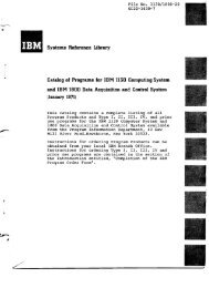
⏐ρ⏐ ⏐ρ⏐ φ 1 0.9 0.8 0.7 0.6 1.0 0.9 0.8 0.3 0.7 0.6 ⏐ρ⏐ 0.5 0.4 0.3 0.2 0.1 0 0 30 60 90 120 150 180 210 240 270 300 330 360 φ 0.4 0.5 Figure 2. Origin of reflectance curves versus variable. + E S Z S N k N 1 1 2 jX Z L ⎛ A B⎞ ⎛ 1 jX ⎞ ⎜ ⎟ ⎜ ⎟ ⎝ C D⎠ ⎝ 0 1 ⎠ N 2 Z 1 1 2 1 2 jB ⎛ 1 0⎞ ⎜ ⎟ ⎝ jB 1⎠ 1 ⎛ t ⎜ ⎝ 0 N 3 2 t:1 0 ⎞ ⎛ cosθ −1 ⎟ ⎜ t ⎠ ⎝ jY0 sinθ N 4 1 2 Z 0 θ Figure 3. Interfaces for lossless subnetworks. jZ0sin θ⎞ ⎟ cos θ ⎠ Typical reflectance cross sections versus a series inductance are shown in Figure 4. The curves at each frequency are similar to segments of the φ curve in Figure 2 except for the skewing in the abscissa. The envelope is defined to be the worst-case reflectance and is composed of piecewise arcs; the derivative of the envelope is discontinuous where the arc segments join. Broadband matching problem (3) is solved by finding the element values in vector x for the common minima on their respective envelopes and varying that x to obtain the lowest-possible minimum reflectance. Further consideration of Figure 4 shows that additional passband frequency samples would interpolate between reflectance curves at adjacent frequencies and only more precisely define the envelope, so choice of samples is not critical. It is important to observe the reflectance curves for ω = 0.4, 0.5, and 0.6 rad/s in Figure 4. They are still just segments of the φ curve in Figure 2, and it is not unusual for all sample frequencies to produce a monotonic (no minimum) envelope as opposed to a unimodal envelope for certain element variables. If only those three particular frequencies in Figure 4 are considered, the series branch would be unnecessary and would be removed (L=0) under the condition that no other elements were changed. Figure 4. Typical reflectances versus a series branch inductance. Each normalized frequency curve is a skewed segment of the curve in Figure 2. 3. DIRECT SEARCH The precise search described in Section 4 removes all unnecessary elements but must be started from an approximate solution to (3). Also, there may be many local minima of (3), especially when unnecessary elements are present. Classical insertion loss theory and other broadband techniques indicate that each element in vector x will be in the range 1/25≤x j ≤25 for sampled data and equalizers normalized to one ohm and one rad/s. Normalized L, C, t, and Z 0 values are explored within that range; only one L or C is varied in traps, the other C or L being dependent on a fixed null frequency. Well-scaled mapping functions are used to relate transmission line lengths to the x j range, which is in turn mapped to log space; see Figure 4. A typical nonsmooth surface at one frequency for two of many variables is shown in Figure 5; all sections resemble Figure 4. An efficient direct search technique for locating the global 23.7 0.226 C 2 22.6 C 3 0.237 1 C 3 C 2 0.499 ρ 22.6 0.5 0.9 0.8 0.7 0.75 0.9 0.6 0.85 0 0.85 C 2 0.5 0.75 0.95 0.7 0.85 0.65 0.9 0.95 0.9 0.8 0.95 0.5 1 1 0.5 0 0.5 1 23.7 0.226 0.237 Figure 5. A typical envelope surface for two variables. minimum is to evaluate the envelope surface at a pattern of points in variable log space. Figure 6 shows such a pattern, which can be considered an archeological grid over the terrain in Figure 5. During a search iteration, each grid point defines a set of element values, and the worst reflectance over all frequency samples determines the envelope surface value. Some point in the pattern will have the least worst-case reflectance, so the pattern is recentered on that point for another iteration. When a better point cannot be found, the pattern granularity (point spacing) is reduced by factor 4, and the search is restarted. A noncritical choice is to center the initial grid on unity; then only three reductions in granularity are required, a total factor of 1/64. The number of pattern trial points is decreased as the 1 0.9 C 3 0.85 V-402
number of equalizer elements increases from 2 to 10 so that about 1000 envelope surface evaluations are required for each iteration. Also, there are many programming strategies for improving search efficiency. 0.8 0.75 0.7 ω =1.0 Optimal Inductance 10 Base Point 0.65 0.9 0.8 BRANCH 2 1 0.1 0.1 1 10 BRANCH 1 Reflection Magnitude 0.6 0.55 0.5 0.45 0.4 0.35 0.3 0.7 0.6 0.4 0.5 Figure 6. A 5×5 lattice (grid) for two variables. 0.3 It has been shown that this grid search converges unfailingly to a point where the surface is nondifferentiable or the gradient is zero [4]. This grid search in log space also avoids local minima that sometimes occur in coordinate sections related to transmission-line variables and avoids the local minima that are usually observed on the principal diagonals of the pattern hypercube in n space. Examination of cross sections and diagonals for many realistic matching data sets and topologies has shown it reasonable to expect the reflectance envelope minimum found to be global. 4. CONSTRAINED GRADIENT OPTIMIZATION The broadband matching objective in (3) is nonsmooth with discontinuous derivatives. Generally, direct searches do not require derivatives to exist, but are known to have very slow final convergence. However, gradient search based on first partial derivatives usually converges rapidly to a nearby minimum. Therefore, (3) is converted to an equivalent differentiable optimization problem by adding one more variable, x n+1 , to the x vector: ( ω ) Min x xn subject to + 1 ρ x , i ≤ x n + 1 , i = 1 m. (4) This objective function is linear, and the m inequality reflectance constraints are differentiable functions. The envelope minimum in Figure 4 is enlarged in Figure 7. It is seen that x n+1 has been reduced to 0.50 with the variable for the inductance having the value 0.72. Also, this solution is determined by binding constraints at 0.3, 0.4, 0.5, 0.8, and 1.0 rad/s; the remaining three constraints are not binding. The standard constrained optimization problem in (4) can be solved by several methods. The Lagrange multiplier method is a precise and rapidly convergent gradient algorithm that is reliable when started near a minimum [2]; it replaces (4) with 0.5 0.6 0.7 0.8 0.9 1 Branch 5 Inductance (henrys) Figure 7. Details of binding reflectances in Figure 4. [ ( x i) x n + 1 + u i ] Min m x xn + 1 + ∑ s i = i max ρ , ω − , 0 2 . (5) 1 The formulation in (5) introduces m pairs of weights, s i , and offsets, u i . The u i offset the origins of the constraints so that the s i weights need not become infinite as with ordinary penalty function optimizers [2]. A particularly simple Lagrange multiplier algorithm [5] starts with the x vector from the grid search and x n+1 set to the maximum reflectance, all s i =1, and all u i =0. There are two loops: The outer loop adjusts the s i and u i based on how the worst-case binding constraint increased or decreased. The inner loop obtains the minimum in (5) with fixed values of s i and u i ; first derivatives are continuous. The inner loop is an unconstrained minimization except for element bounds or holds, requires first partial derivatives, and converges at a quadratic rate. The outer loop is an approximate minimizer that converges at a linear rate [2]. The minimum reflectance is obtained subject to the binding constraints within a few iterations; see Figure 7. Significantly, the m s i ×u i products at the constrained minimum are equal to the Lagrange multipliers associated with (4); that is one basis for adjusting the s i and u i values in the outer loop. The gradient search is also conducted in variable log space, which guarantees positive element values and normalizes the derivatives for optimal scaling. The grid search requires several thousand evaluations of reflectance, and the Lagrange multiplier method requires reflectances and their first partial derivatives with respect to each component of x. Fortunately, these values can be obtained exactly with great efficiency using the element ABCD parameters in Figure 3 [6]. A special advantage of GRABIM is that the overall equalizer ABCD parameters at each frequency need be computed only once. Therefore, sets of Z L and Z S data defining V-403
Page 1: ISCAS 2000 - IEEE International Sym

Cuthbert, 2000 - IEEE Global History Network

Create successful ePaper yourself

Delete template?

Save as template?