Cuthbert, 2000 - IEEE Global History Network
Cuthbert, 2000 - IEEE Global History Network
Cuthbert, 2000 - IEEE Global History Network

You also want an ePaper? Increase the reach of your titles
YUMPU automatically turns print PDFs into web optimized ePapers that Google loves.
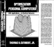
ISCAS <strong>2000</strong> - <strong>IEEE</strong> International Symposium on Circuits and Systems, May 28-31, <strong>2000</strong>, Geneva, Switzerland<br />
A REAL FREQUENCY TECHNIQUE OPTIMIZING<br />
BROADBAND EQUALIZER ELEMENTS<br />
Thomas R. <strong>Cuthbert</strong>, Jr., Ph.D.<br />
Greenwood, Arkansas 72936, USA<br />
trcpep@aol.com<br />
ABSTRACT<br />
A practical real frequency technique for broadband impedance<br />
matching is based on bilinear reflection behavior versus lumped<br />
and distributed element variables. An efficient grid search<br />
locates a likely-global solution so that a precise constrained<br />
gradient optimization can eliminate unnecessary elements in<br />
candidate networks.<br />
1. INTRODUCTION<br />
Broadband matching requires a lossless two-port matching<br />
network (equalizer) to minimize the maximum loss at passband<br />
frequencies. Usually the load and/or source are not pure<br />
resistances. See Figure 1; the maximum available source power is<br />
P as =⎥E S ⎜ 2 /4R S , where Z S ≡R S +jX S . The relative power delivered<br />
to the load, Z L , at a given frequency is<br />
P L<br />
T ≡ = 1 −<br />
P aS<br />
The generalized reflection coefficient is<br />
2<br />
ρ in . (1)<br />
Z S<br />
1 2<br />
E S<br />
LOSSLESS<br />
MATCHING<br />
NETWORK<br />
Z L<br />
ρ in<br />
Figure 1. Broadband matching network terminations.<br />
*<br />
Z in − Z S<br />
ρ in ≡ . (2)<br />
Z in + Z S<br />
Reflectance is reflection magnitude at a given frequency and is<br />
constant at all two-port interfaces because of conservation of<br />
power. The minimax objective in broadband matching is<br />
Min<br />
x<br />
⎡<br />
⎣<br />
⎢<br />
( ω) ≡<br />
Max<br />
ρ( x ω)<br />
f x, , ,<br />
ω ⎥<br />
x ∈R n , ω<br />
1<br />
≤ω≤ωm<br />
;<br />
n is the number of degrees of freedom in the equalizer, i.e., the<br />
element values, and m passband frequencies are selected.<br />
Two broadband matching techniques are classical insertion loss<br />
theory and real frequency techniques (RFT) [1]. The former is<br />
applicable to very few practical matching problems. The RFT is<br />
⎤<br />
⎦<br />
(3)<br />
a numerical optimization method that is applicable to a wide<br />
range of practical problems, and utilizes frequency-sampled load<br />
and/or source impedance data. Numerical optimization adjusts<br />
free parameters (variables) to minimize an objective function,<br />
e.g. least squares [2] or random search [3]. A well-known RFT<br />
employs one or more approximation and optimization stages and<br />
ends with polynomial synthesis [1]. The variables are<br />
polynomial coefficients or s-plane root coordinates, so parts of<br />
that process are extremely ill-conditioned [6].<br />
This paper describes a well-conditioned RFT with an<br />
optimization objective that depends on variables in simple ways,<br />
leading to likely-global optimal results. The variables are values<br />
of equalizer elements, which may be mixed lumped and<br />
distributed. This new technique avoids linear, nonlinear, or<br />
rational approximations and polynomial synthesis. An optimal<br />
equalizer topology is not known in advance; otherwise, some<br />
common optimization algorithms might find optimal solutions.<br />
Here a useful candidate equalizer topology is selected, and the<br />
grid approach to broadband impedance matching (GRABIM)<br />
automatically eliminates all unnecessary elements. The theory is<br />
discussed, the two optimization stages are described, a well<br />
known example is solved, and references are provided.<br />
2. REFLECTION CHARACTERISTICS<br />
The GRABIM technique utilizes a candidate equalizer topology<br />
with vector x=[x j ] containing all the variable element values and<br />
operates on the reflectance at each passband frequency versus<br />
each element value, x j , j=1…n. Choose m≈2n passband<br />
frequencies, ω i , i=1…m, each associated with data constants for<br />
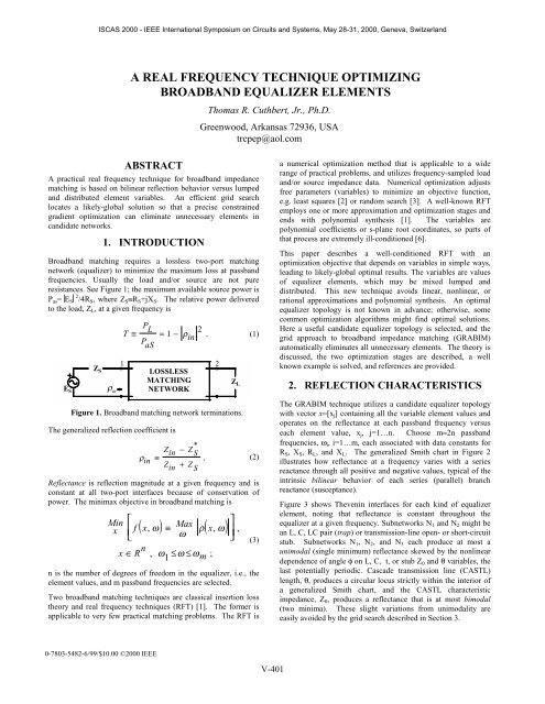
R S , X S , R L , and X L . The generalized Smith chart in Figure 2<br />
illustrates how reflectance at a frequency varies with a series<br />
reactance through all positive and negative values, typical of the<br />
intrinsic bilinear behavior of each series (parallel) branch<br />
reactance (susceptance).<br />
Figure 3 shows Thevenin interfaces for each kind of equalizer<br />
element, noting that reflectance is constant throughout the<br />
equalizer at a given frequency. Subnetworks N 1 and N 2 might be<br />
an L, C, LC pair (trap) or transmission-line open- or short-circuit<br />
stub. Subnetworks N 1 , N 2 , and N 3 each produce at most a<br />
unimodal (single minimum) reflectance skewed by the nonlinear<br />
dependence of angle φ on L, C, t, or stub Z 0 and θ variables, the<br />
last potentially periodic. Cascade transmission line (CASTL)<br />
length, θ, produces a circular locus strictly within the interior of<br />
a generalized Smith chart, and the CASTL characteristic<br />
impedance, Z 0 , produces a reflectance that is at most bimodal<br />
(two minima). These slight variations from unimodality are<br />
easily avoided by the grid search described in Section 3.<br />
0-7803-5482-6/99/$10.00 ©<strong>2000</strong> <strong>IEEE</strong><br />
V-401
⏐ρ⏐<br />
⏐ρ⏐<br />
φ<br />
1<br />
0.9<br />
0.8<br />
0.7<br />
0.6<br />
1.0<br />
0.9<br />
0.8<br />
0.3<br />
0.7<br />
0.6<br />
⏐ρ⏐<br />
0.5<br />
0.4<br />
0.3<br />
0.2<br />
0.1<br />
0<br />
0 30 60 90 120 150 180 210 240 270 300 330 360<br />
φ<br />
0.4<br />
0.5<br />
Figure 2. Origin of reflectance curves versus variable.<br />
+<br />
E S<br />
Z S<br />
N k<br />
N 1<br />
1 2<br />
jX<br />
Z L<br />
⎛ A B⎞<br />
⎛ 1 jX ⎞<br />
⎜ ⎟ ⎜ ⎟<br />
⎝ C D⎠<br />
⎝ 0 1 ⎠<br />
N 2<br />
Z 1<br />
1 2<br />
1 2<br />
jB<br />
⎛ 1 0⎞<br />
⎜ ⎟<br />
⎝ jB 1⎠<br />
1<br />
⎛ t<br />
⎜<br />
⎝ 0<br />
N 3<br />
2 t:1<br />
0 ⎞ ⎛ cosθ<br />
−1 ⎟ ⎜<br />
t ⎠ ⎝ jY0<br />
sinθ<br />
N 4<br />
1 2<br />
Z 0 θ<br />
Figure 3. Interfaces for lossless subnetworks.<br />
jZ0sin<br />
θ⎞<br />
⎟<br />
cos θ ⎠<br />
Typical reflectance cross sections versus a series inductance are<br />
shown in Figure 4. The curves at each frequency are similar to<br />
segments of the φ curve in Figure 2 except for the skewing in the<br />
abscissa. The envelope is defined to be the worst-case reflectance<br />
and is composed of piecewise arcs; the derivative of the envelope<br />
is discontinuous where the arc segments join. Broadband<br />
matching problem (3) is solved by finding the element values in<br />
vector x for the common minima on their respective envelopes<br />
and varying that x to obtain the lowest-possible minimum<br />
reflectance. Further consideration of Figure 4 shows that<br />
additional passband frequency samples would interpolate<br />
between reflectance curves at adjacent frequencies and only more<br />
precisely define the envelope, so choice of samples is not critical.<br />
It is important to observe the reflectance curves for ω = 0.4, 0.5,<br />
and 0.6 rad/s in Figure 4. They are still just segments of the φ<br />
curve in Figure 2, and it is not unusual for all sample frequencies<br />
to produce a monotonic (no minimum) envelope as opposed to a<br />
unimodal envelope for certain element variables. If only those<br />
three particular frequencies in Figure 4 are considered, the series<br />
branch would be unnecessary and would be removed (L=0)<br />
under the condition that no other elements were changed.<br />
Figure 4. Typical reflectances versus a series branch<br />
inductance. Each normalized frequency curve is a<br />
skewed segment of the curve in Figure 2.<br />
3. DIRECT SEARCH<br />
The precise search described in Section 4 removes all<br />
unnecessary elements but must be started from an approximate<br />
solution to (3). Also, there may be many local minima of (3),<br />
especially when unnecessary elements are present. Classical<br />
insertion loss theory and other broadband techniques indicate<br />
that each element in vector x will be in the range 1/25≤x j ≤25 for<br />
sampled data and equalizers normalized to one ohm and one<br />
rad/s. Normalized L, C, t, and Z 0 values are explored within that<br />
range; only one L or C is varied in traps, the other C or L being<br />
dependent on a fixed null frequency. Well-scaled mapping<br />
functions are used to relate transmission line lengths to the x j<br />
range, which is in turn mapped to log space; see Figure 4.<br />
A typical nonsmooth surface at one frequency for two of many<br />
variables is shown in Figure 5; all sections resemble Figure 4.<br />
An efficient direct search technique for locating the global<br />
23.7<br />
0.226<br />
C 2<br />
22.6<br />
C 3<br />
0.237<br />
1<br />
C 3<br />
C 2<br />
0.499<br />
ρ<br />
22.6<br />
0.5<br />
0.9<br />
0.8<br />
0.7<br />
0.75<br />
0.9<br />
0.6 0.85<br />
0<br />
0.85<br />
C 2<br />
0.5 0.75 0.95<br />
0.7<br />
0.85 0.65 0.9<br />
0.95<br />
0.9 0.8<br />
0.95<br />
0.5<br />
1<br />
1 0.5 0 0.5 1<br />
23.7<br />
0.226<br />
0.237<br />
Figure 5. A typical envelope surface for two variables.<br />
minimum is to evaluate the envelope surface at a pattern of<br />
points in variable log space. Figure 6 shows such a pattern,<br />
which can be considered an archeological grid over the terrain in<br />
Figure 5. During a search iteration, each grid point defines a set<br />
of element values, and the worst reflectance over all frequency<br />
samples determines the envelope surface value. Some point in<br />
the pattern will have the least worst-case reflectance, so the<br />
pattern is recentered on that point for another iteration.<br />
When a better point cannot be found, the pattern granularity<br />
(point spacing) is reduced by factor 4, and the search is restarted.<br />
A noncritical choice is to center the initial grid on unity; then<br />
only three reductions in granularity are required, a total factor of<br />
1/64. The number of pattern trial points is decreased as the<br />
1<br />
0.9<br />
C 3<br />
0.85<br />
V-402
number of equalizer elements increases from 2 to 10 so that<br />
about 1000 envelope surface evaluations are required for each<br />
iteration. Also, there are many programming strategies for<br />
improving search efficiency.<br />
0.8<br />
0.75<br />
0.7<br />
ω =1.0<br />
Optimal<br />
Inductance<br />
10<br />
Base Point<br />
0.65<br />
0.9<br />
0.8<br />
BRANCH 2<br />
1<br />
0.1<br />
0.1 1 10<br />
BRANCH 1<br />
Reflection Magnitude<br />
0.6<br />
0.55<br />
0.5<br />
0.45<br />
0.4<br />
0.35<br />
0.3<br />
0.7<br />
0.6<br />
0.4<br />
0.5<br />
Figure 6. A 5×5 lattice (grid) for two variables. 0.3<br />
It has been shown that this grid search converges unfailingly to a<br />
point where the surface is nondifferentiable or the gradient is<br />
zero [4]. This grid search in log space also avoids local minima<br />
that sometimes occur in coordinate sections related to<br />
transmission-line variables and avoids the local minima that are<br />
usually observed on the principal diagonals of the pattern<br />
hypercube in n space. Examination of cross sections and<br />
diagonals for many realistic matching data sets and topologies<br />
has shown it reasonable to expect the reflectance envelope<br />
minimum found to be global.<br />
4. CONSTRAINED GRADIENT<br />
OPTIMIZATION<br />
The broadband matching objective in (3) is nonsmooth with<br />
discontinuous derivatives. Generally, direct searches do not<br />
require derivatives to exist, but are known to have very slow final<br />
convergence. However, gradient search based on first partial<br />
derivatives usually converges rapidly to a nearby minimum.<br />
Therefore, (3) is converted to an equivalent differentiable<br />
optimization problem by adding one more variable, x n+1 , to the x<br />
vector:<br />
( ω )<br />
Min<br />
x xn subject to<br />
+ 1<br />
ρ x , i ≤ x n + 1<br />
, i = 1 m.<br />
(4)<br />
This objective function is linear, and the m inequality reflectance<br />
constraints are differentiable functions.<br />
The envelope minimum in Figure 4 is enlarged in Figure 7. It is<br />
seen that x n+1 has been reduced to 0.50 with the variable for the<br />
inductance having the value 0.72. Also, this solution is<br />
determined by binding constraints at 0.3, 0.4, 0.5, 0.8, and 1.0<br />
rad/s; the remaining three constraints are not binding. The<br />
standard constrained optimization problem in (4) can be solved<br />
by several methods. The Lagrange multiplier method is a precise<br />
and rapidly convergent gradient algorithm that is reliable when<br />
started near a minimum [2]; it replaces (4) with<br />
0.5 0.6 0.7 0.8 0.9 1<br />
Branch 5 Inductance (henrys)<br />
Figure 7. Details of binding reflectances in Figure 4.<br />
[ ( x i)<br />
x n + 1<br />
+ u i ]<br />
Min m<br />
x xn + 1<br />
+ ∑ s<br />
i = i max ρ , ω − , 0 2<br />
. (5)<br />
1<br />
The formulation in (5) introduces m pairs of weights, s i , and<br />
offsets, u i . The u i offset the origins of the constraints so that the<br />
s i weights need not become infinite as with ordinary penalty<br />
function optimizers [2].<br />
A particularly simple Lagrange multiplier algorithm [5] starts<br />
with the x vector from the grid search and x n+1 set to the<br />
maximum reflectance, all s i =1, and all u i =0. There are two loops:<br />
The outer loop adjusts the s i and u i based on how the worst-case<br />
binding constraint increased or decreased. The inner loop<br />
obtains the minimum in (5) with fixed values of s i and u i ; first<br />
derivatives are continuous. The inner loop is an unconstrained<br />
minimization except for element bounds or holds, requires first<br />
partial derivatives, and converges at a quadratic rate. The outer<br />
loop is an approximate minimizer that converges at a linear rate<br />
[2]. The minimum reflectance is obtained subject to the binding<br />
constraints within a few iterations; see Figure 7. Significantly,<br />
the m s i ×u i products at the constrained minimum are equal to the<br />
Lagrange multipliers associated with (4); that is one basis for<br />
adjusting the s i and u i values in the outer loop. The gradient<br />
search is also conducted in variable log space, which guarantees<br />
positive element values and normalizes the derivatives for<br />
optimal scaling.<br />
The grid search requires several thousand evaluations of<br />
reflectance, and the Lagrange multiplier method requires<br />
reflectances and their first partial derivatives with respect to each<br />
component of x. Fortunately, these values can be obtained<br />
exactly with great efficiency using the element ABCD parameters<br />
in Figure 3 [6]. A special advantage of GRABIM is that the<br />
overall equalizer ABCD parameters at each frequency need be<br />
computed only once. Therefore, sets of Z L and Z S data defining<br />
V-403
neighborhoods of uncertain impedance at each frequency also<br />
can be broadband matched efficiently.<br />
5. EXAMPLE<br />
There is a double-match example that cannot be solved by the<br />
classical insertion loss method [7]. The source and load models<br />
shown in Figure 8 are seldom known; however, their impedance<br />
data in the desired passband from 0.3 to 1.0 rad/s in 0.1 intervals<br />
are assumed given. The source resistance being zero at 1.29 rad/s<br />
is particularly difficult. The RFT method in [7] utilizes several<br />
arbitrary approximations, optimizations, and synthesis steps to<br />
yield a six-element equalizer with passband loss 0.85 to 1.42 dB.<br />
1.0<br />
0.75<br />
0.3 2.0 LOSSLESS<br />
E 4<br />
S EQUALIZER<br />
Figure 8. A difficult broadband matching problem.<br />
The GRABIM technique used the same data and a six- element<br />
equalizer topology consisting of a Pi of L’s at the source<br />
followed by a Pi of C’s at the load. (The source is capacitive and<br />
the load is inductive; Pi networks implicitly contain ideal<br />
transformers.) The grid search required 7026 network analyses<br />
performed in 2 seconds by a 200 MHz PC; the worst-case<br />
insertion loss was reduced to 2.6 dB. A few Lagrange multiplier<br />
loops reduced the loss to 1.24 dB while automatically removing<br />
one L and one C. See Figure 9(a); two other solutions started<br />
from other topologies also are shown in Figures 9(b) and 9(c).<br />
(a) Best case found:<br />
0.97 < S 21 dB < 1.24<br />
(b) Five branch bandpass:<br />
1.21 < S 21 dB < 1.63<br />
(c) Five branch highpass:<br />
0.88 < S 21 dB < 1.75<br />
0.56<br />
0.72<br />
0.85<br />
0.68<br />
(a)<br />
(b)<br />
4.34<br />
(c)<br />
7.84<br />
4.00<br />
2.26<br />
2.37<br />
2.34<br />
1.07<br />
2.45<br />
1.40<br />
Figure 9. Three full-rank broadband network solutions.<br />
1<br />
8.92<br />
6. SUMMARY<br />
The GRABIM RFT is a pure numerical optimization algorithm<br />
that is fast, simple, and reliable. It solves double-match problems<br />
as easily as single-match problems. GRABIM locates a likelyglobal<br />
optimal solution for a given topology and eliminates<br />
unnecessary branches during a two-stage process of optimizing<br />
equalizer elements. Mixed lumped and distributed elements are<br />
allowed, based on clearly defined behavior of reflection<br />
magnitude versus element variables. Inexpensive, documented<br />
software is available from the author.<br />
GRABIM features:<br />
• Measured single- or double-match source and load<br />
impedance data at sampled passband frequencies,<br />
• Noncritical choice of frequency samples,<br />
• Mixed lumped/distributed equalizer elements,<br />
• Bandpass or lowpass equalizers,<br />
• Arbitrary or stored candidate topologies of varying degree,<br />
• Automatic elimination of unnecessary elements,<br />
• No element initial values required,<br />
• Bounds or holds on element values,<br />
• Efficient broadband matching of impedance neighborhoods,<br />
• Likely-global optimal solutions, and<br />
• Proven, well-conditioned numerical techniques.<br />
7. REFERENCES<br />
[1] Carlin, H. J. and P. P. Civalleri (1998). Wideband Circuit<br />
Design. NY: CRC Press.<br />
[2] Fletcher, R. (1980-1981). Practical Methods of Optimization:<br />
Unconstrained Optimization, Vol. 1, and<br />
Constrained Optimization, Vol. 2. NY: John Wiley.<br />
[3] Dedieu, H., C. Dehollain, J. Neirynck, and G. Rhodes<br />
(1994). A new method for solving broadband matching<br />
problems. <strong>IEEE</strong> Trans. Circuits and Sys., V41, N9.<br />
Sept.:561-571.<br />
[4] Torczon, V. (1991). On the convergence of the multidirectional<br />
search algorithm. SIAM J. Opti., V1, N1.<br />
Feb.:123-145.<br />
[5] Powell, M. J. D. (1969). A method for nonlinear constraints<br />
in minimization problems, in Optimization, R. Fletcher, Ed.<br />
NY: Academic Press, pp. 283-297.<br />
[6] Orchard, H. J. (1985). Filter design by iterated analysis.<br />
<strong>IEEE</strong> Trans. Circuits & Sys., V32, N11. Nov.:1089-96.<br />
[7] Yarman, B. S. and A. Fettweis (1990). Computer-aided<br />
double matching via parametric representation of Brune<br />
functions. <strong>IEEE</strong> Trans. Circuits & Sys., V37, N2. Feb.:212-<br />
222.<br />
V-404