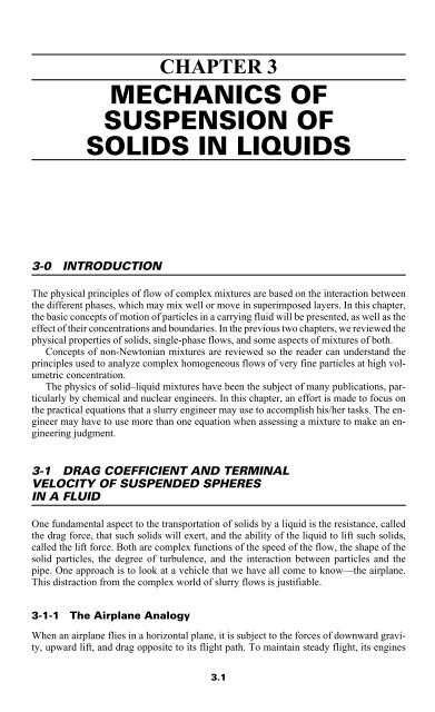
CHAPTER 3 MECHANICS OF SUSPENSION OF SOLIDS IN LIQUIDS

CHAPTER 3
MECHANICS OF
SUSPENSION OF
SOLIDS IN LIQUIDS
3-0 INTRODUCTION
The physical principles of flow of complex mixtures are based on the interaction between
the different phases, which may mix well or move in superimposed layers. In this chapter,
the basic concepts of motion of particles in a carrying fluid will be presented, as well as the
effect of their concentrations and boundaries. In the previous two chapters, we reviewed the
physical properties of solids, single-phase flows, and some aspects of mixtures of both.
Concepts of non-Newtonian mixtures are reviewed so the reader can understand the
principles used to analyze complex homogeneous flows of very fine particles at high volumetric
concentration.
The physics of solid–liquid mixtures have been the subject of many publications, particularly
by chemical and nuclear engineers. In this chapter, an effort is made to focus on
the practical equations that a slurry engineer may use to accomplish his/her tasks. The engineer
may have to use more than one equation when assessing a mixture to make an engineering
judgment.
3-1 DRAG COEFFICIENT AND TERMINAL
VELOCITY OF SUSPENDED SPHERES
IN A FLUID
One fundamental aspect to the transportation of solids by a liquid is the resistance, called
the drag force, that such solids will exert, and the ability of the liquid to lift such solids,
called the lift force. Both are complex functions of the speed of the flow, the shape of the
solid particles, the degree of turbulence, and the interaction between particles and the
pipe. One approach is to look at a vehicle that we have all come to know—the airplane.
This distraction from the complex world of slurry flows is justifiable.
3-1-1 The Airplane Analogy
When an airplane flies in a horizontal plane, it is subject to the forces of downward gravity,
upward lift, and drag opposite to its flight path. To maintain steady flight, its engines
3.1

3.2 CHAPTER THREE
must develop sufficient thrust to overcome drag. The airplane must also fly above its
stalling speed.
The lift and drag are aerodynamic forces (Figure 3-1). They are proportional to the
surface area, the density of air, the inclination of the airplane body with respect to speed,
and the square of the speed. For the airplane wing, these forces are expressed as
L = 0.5 CL�V 2Sw (3-1)
D = 0.5 CD�V 2Sw (3-2)
where
� = density of the fluid
V = cruising speed of airplane
CL = lift coefficient of wing airfoil
CD = drag coefficient of wing airfoil
The aerodynamic drag consists of two components: the profile drag and induced drag.
The induced drag is proportional to the square of the lift. Airfoils are designed to maximize
the lift-to-drag ratio, or to develop the most lift at the least drag penalty:
2 CD = CD0 + kwC L (3-3)
where
CD0 = the profile drag
kw = a function of the shape of the wing (minimum for an elliptical wing and for a wing
flying in ground effect)
The value of the drag and lift coefficients are determined by the shape of the flying ob-
Thrust
Wing lift
Weight
Forces on an aircraft in
steady horizontal flight
Drag
Stabilizer lift
Weight
Thrust
Drag
Forces on a rocket in
vertical flight
FIGURE 3-1 Lift and drag forces on moving objects.
Buoyancy
Drag
Weight
Forces on a free-falling
particle immersed in a fluid

MECHANICS OF SUSPENSION OF SOLIDS IN LIQUIDS
ject, but also by the physical properties of a fluid, particularly the density, viscosity, and
speed of motion. Nondimensional analysis, an important branch of fluid dynamics, allows
the expression of these relationships by characteristic numbers. The Reynolds Number
has already introduced in Chapter 2.
For an airplane in a steady horizontal linear flight, the lift must overcome weight and
the thrust drag. A rocket flying in a vertical plane must develop sufficient thrust to overcome
drag forces as well as weight:
L = W and T = D For an Airplane
T = W + D For a rocket in vertical flight
3-1-2 Buoyancy of Floating Objects
The principle of Archimedes is well known. It states that the buoyancy force developed
by an object static in a fluid is equal to the weight of liquid of equivalent volume occupied
by the object. When the density of the object is less than the density of the liquid, the object
floats, and in the inverse situation, the object sinks.
For a sphere immersed in a fluid of density �L, the buoyancy force is calculated from
the weight of fluid the particle displaces:
3 FBF = (�/6)d g�Lg (3-4)
where
FBF = buoyancy force
dg = sphere diameter
g = acceleration due to gravity (9.78–9.81 m/s2 )
3-1-3 Terminal Velocity of Spherical Particles
Although most solids are not spherical in shape, the sphere is the point of reference for
the analysis of irregularly shaped solids.
3-1-3-1 Terminal Velocity of a Sphere Falling in a Vertical Tube
When a sphere is allowed to fall freely in a tube, the buoyancy and the drag forces act vertically
upward, whereas the weight force acts downward. At the terminal or free settling
velocity, in the absence of any centrifugal, electrostatic, or magnetic forces
W = D + FBF (3-5)
� �dg 3�Sg = � �dg 3 2
� �
�d
2 g
�Lg + 0.5 CD�LV t� � (3-6)
�
6
�
6
�
4
The drag coefficient corresponding to free fall of the particle is calculated as
4(�S – �L)gdg CD = ��
(3-7)
3�LV t 2
where
d g = sphere diameter
g = acceleration due to gravity, typically 9.8 m/s 2 or 32.2 ft/sec 2
3.3

3.4 CHAPTER THREE
Vt = the terminal (or free settling) speed
�s = the density of the solid sphere in kg/m3 or slugs/ft3 �L = the density of the liquid
The terminal (or sinking) velocity is measured using a visual accumulation tube with a
recording drum. Various mathematical models have been derived for the drag coefficient.
Turton and Levenspiel (1986) proposed the following equation:
0.413
0.657 CD = (1 + 0.173Re p ) ���
(3-8)
1 + 1.163 × 104 24
� –1.09
Rep
Re p
Example 3-1
Using the Turton and Levenspiel equation, write a small computer program in quickbasic
to tabulate the drag coefficient of a sphere.
LPRINT “ Drag coefficient vs. Reynolds Number based on
Turton, R., and O. Levenspiel”
RE0= 1
15 FOR I=1 TO 10
RE=I*RE0
CD= (24/RE) * (1+0.173*RE^0.657)*(0.413/(1+11630*RE^-1.09)
PRINT USING “RE= ###### ; Cd = ##.#### “; RE,CD
NEXT I
IF RE>1E6 THEN GOTO 30
RE0=RE
TABLE 3-1 Particle Reynolds Number and Corresponding Drag Coefficient for a
Sphere Based on the Equation of Turton and Levenspiel (1986) as per Example 3-1
Particle Drag Particle Drag Particle Drag
Reynolds coefficient, Reynolds coefficient, Reynolds coefficient,
number, Rep CD number, Rep CD number, Rep CD 1 28.1520 80 1.2266 6000 0.3983
2 15.2735 90 1.1571 7000 0.4042
3 10.8485 100 1.0994 8,000 0.4151
4 8.5809 200 0.5025 9,000 0.4151
5 7.1908 300 0.6793 10,000 0.4200
6 6.2459 400 0.6085 20,000 0.4497
7 5.5588 500 0.5617 30,000 0.4617
8 5.0349 600 0.5281 40,000 0.4671
9 4.6211 700 0.5029 50,000 0.4697
10 4.2851 800 0.4832 60,000 0.4709
20 2.6866 900 0.4675 70,000 0.4713
30 2.0940 1,000 0.4547 80,000 0.4713
40 1.7729 2,000 0.3990 90,000 0.4711
50 1.5670 3,000 0.3878 100,000 0.4707
60 1.4216 4,000 0.3883 200,000 0.4653
70 1.3124 5,000 0.3927 300,000 0.4609

Drag Coefficient C D
25
20
15
10
5
GOTO 15
30 END
0
0 2 4 6 8 10
Rep
MECHANICS OF SUSPENSION OF SOLIDS IN LIQUIDS
30 0
C D
C D
0
6
4
2
1.2
1.0
0.8
0.6
0.4
0.2
20
200
40
400
Results are tabulated in Table 3-1 and presented in Figure 3-2 in a linear scale rather
than a logarithmic scale. Linear scales are sometimes more useful to the mine operator
who is in a remote area and has little time to waste on difficult logarithmic graphs
3-1-3-2 Very Fine Spheres
For small particles in the range of a diameter d50 < 0.15 mm (0.0059 in), the most common
equation was created by Stokes and reported by Herbich (1991) and Wasp et al. (1977),
who indicate that the main forces are due to the viscosity effect in the laminar flow regime:
D = 3��dg (3-9)
In the laminar regime, the drag coefficient is inversely proportional to the Reynolds number,
i.e., CD = 24/Rep. The terminal velocity is expressed by Stoke’s equation:
2 (�S – �L)d gg Vt = ��
(3-10)
18�L�
Stokes’s equation is limited to particle Reynolds numbers smaller than 0.1, but has often
been used for particle Reynolds Numbers as large as 1 (based on sphere diameter d g).
60
600
80
800
100
Rep
3
10
Rep
CD CD D C
FIGURE 3-2 Drag coefficient of a sphere for Reynolds number smaller than 300,000.
0.6
0.4
0.2
0
0.6
0.4
0.2
0
0.6
0.4
0.2
1X10 5
2000
4
2X10
4000
4
4X10
Rep
5
3X10
6000
4
6X10
8000
4
8X10
3.5
10 4
Rep
5
1X10
Rep

3.6 CHAPTER THREE
From Equation 3-10, Herbich (1968) pointed out that the radius of particles for which the
validity of the equation is in doubt is expressed as
4.5� 2 � L
� (�S – � L)
R = � � 3/2
This equation is not set in stone for all situations. Rubey (1933) demonstrated one example
by showing that Stoke’s law does not apply to spherical quartz suspended in water
when the particle diameter exceeds 0.014 mm (0.00055 in, mesh 105).
3-1-3-3 Intermediate Spheres
For the range of particle Reynolds numbers between 1 and 1000, i.e., when
dpV0 �
1 < � < 1000
�
Govier and Aziz (1972) reported that Allen (1900) derived the following equation:
(� � – � L)g
Vt = 0.2� � 0.72
��
�L
(3-11)
Example 3-2
A slurry mixture consists of fine rocks at an average particle diameter of 140 �m, with a
particle density of 2800 kg/m3 . The carrier liquid is water with a dynamic viscosity of 1.5
× 10 –3 Pa · s. The volumetric concentration of the solids is 12%. Determine the terminal
velocity of the particles.
Solution
Using Equation 1-9, the dynamic viscosity of the mixture is
�m = �L[1 + 2.5C� + 10.05C� 2 + 0.00273 exp(16.6C�)]
= 1.5 × 10 –3 [1 + 2.5 × 0.12 + 10.05(0.12) 2 + 0.00273 exp (16.6 × 0.12)]
�m = 2.197 × 10 –3 Pa · s.
Let us check the magnitude of the Reynolds number:
= = 4.468
The Allen law applies in a transition regime:
Vt = 0.2 [9.81 × 1.8] 0.72
(140 × 10 –6 ) 1.18
���
(2.197 × 10 –3 /2800) 0.45
140 × 10 –6 × 0.02504 × 2800
���
2.197 × 10 –3
d�V0� �
�
2.83 × 10
Vt = 0.2 × 7.903
–5
��
0.001789
V t = 0.02504 m/s
d p 1.18
� (�/�) 0.45
Richards (1908) demonstrated that Stokes’s equation is inaccurate for particles with a
diameter larger than 0.2 mm (0.00787 in, mesh 70) and conducted extensive tests for

MECHANICS OF SUSPENSION OF SOLIDS IN LIQUIDS
quartz particles (with a specific gravity of 2.65) in laminar, transitional, and turbulent
regimes. He derived the following equation for terminal velocity in mm/s:
8.925
Vt = ����
(3-12)
3 1/2 dg{[1 + 95(�S/�L – 1)d g] – 1}
Where dg, the diameter of the sphere, is expressed in mm. This equation covers the range
of particles between 0.15–1.5 mm (0.0059–0.059 in) at particle Reynolds numbers between
10 and 1000.
3-1-3-4 Large Spheres
For particles with a diameter in excess of 1.5 mm, Herbrich (1991) expressed the terminal
velocity by the following equation:
Vt = Kt�[d� ��� g( ��� S/ L�–� 1�)] � (3-13)
where Kt = an experimental constant = 5.45 for Rep > 800, according to Govier and Aziz
(1972).
Equation 3-13 is often called Newton’s law. In the regime of Newton’s law, the drag
coefficient of a sphere is approximately 0.44, as shown in Figure 3-2. Newton’s law applies
to turbulent flow regimes.
Other equations for terminal velocity of particles have been developed by various authors.
Four different equations are presented in Table 3-2.
Example 3-3
Using the Budyruck equation from Table 3-3, determine the terminal velocity of spheres
from 0.1 to1 mm.
A simple computer program is written in quickbasic as follows:
LPRINT
LPRINT “BUDRYCK AND RITTINGER EQUATION FOR TERMINAL
VELOCITY OF SPHERES IN WATER”
LPRINT
LPRINT DP0 = .1
FOR I=1 to 11
DP = I*DP0
VS= (8.925/DP)*(SQR(1+157*DP^30-1)
LPRINT USING “PARTICLE DIAMETER = ##.### mm TERMINAL
VELOCITY Vs = ##.### mm/s”;DP,VS
NEXT I
FOR J=12 TO 20
DP = J*DP0
TABLE 3-2 Equations for Terminal Speed of Large Spheres
Name Equation* Application
Budryck 3 1/2 Vt = 8.925[(1 + 157d g) – 1]/dg For dg < 1.1 mm
Rittinger Vt = 87(1.65dg) 1/2 For 1.2 < dg < 2 mm
*Where V t is expressed in mm/s and d g in mm.
3.7

3.8 CHAPTER THREE
TABLE 3-3 Calculation of Terminal Velocity of Spheres in Accordance with
Budryck’s Equation
Particle diameter Terminal velocity Particle diameter Terminal velocity
dp in mm Vs in mm/s dp in mm Vs in mm/s
0.1 6.75 0.7 81.63
0.2 22.4 0.8 89.49
0.3 38.34 0.9 96.64
0.4 51.85 1.0 103.26
0.5 63.21 1.1 109.45
0.6 73.02
VS= 87*SQR(1.65*DP)
LPRINT USING “PARTICLE DIAMETER = ##.### mm TERMINAL
VELOCITY Vs = ##.### mm/s”;DP,VS
NEXT J
END
The results are shown in Tables 3-3, 3-4, and Figure 3-3
Herbich (1968) measured drag coefficients for ocean nodules to be as high as 0.6 at
particle Reynolds numbers of 200. This high value is reached with spheres at a particle
Reynolds number of 1000.
3-1-4 Effects of Cylindrical Walls on Terminal Velocity
The previous paragraphs focused on the settling velocity of a single particle or widely
separated particles. The presence of a vessel or cylindrical walls tends to multiply the interaction
between particles and cause some collisions. Extensive tests have been conducted
on flows in vertical tubes. Brown and associates (1950) recommended multiplying the
terminal speed of a single particle by a wall correction factor Fw. For laminar flows they
proposed to use the Francis equation:
Fw = 1 – (d�/Di) 9/4 (3-14a)
They proposed to use the Munroe equation for a turbulent flow regime:
Fw = 1 – (d�/Di) 1.5 (3-14b)
where Di = the inner diameter of the tube
TABLE 3-4 Calculation of Terminal Velocity of Spheres in Accordance with
Rittinger’s Equation
Particle diameter Terminal velocity Particle diameter Terminal velocity
d p in mm V t in mm/s d p in mm V t in mm/s
1.1 117.21 1.6 141.36
1.2 122.42 1.7 145.71
1.3 127.42 1.8 149.93
1.4 132.23 1.9 154.04
1.5 136.87 2.0 158.04

in mm/s
Terminal velocity V
t
160
140
120
100
80
60
40
in mm/s
Terminal velocity V
t
MECHANICS OF SUSPENSION OF SOLIDS IN LIQUIDS
120
100
80
60
40
20
0
0 0.01 0.02 0.03 0.04 0.05
Sphere diameter d p in inches
0 0.2 0.4 0.6 0.8 1.0 1.2
Sphere diameter dp
in mm
0.04 0.05 0.06 0.07 0.08
1.0 1.2 1.4 1.6 1.8 2.0
Sphere diameter dp
in mm
(a)
Sphere diameter d p in inches
(b)
5
4
3
2
1
0
Terminal velocity V
t
in inch/sec
6
5
4
3
2
1
3.9
inch /sec
Terminal velocity V
t
in
FIGURE 3-3 Terminal velocity of spheres (a) in accordance with Budryck’s equation, (b) in
accordance with Rittinger’s equation.

3.10 CHAPTER THREE
Example 3-4
The flow described in Example 3-2 occurs in a 63 mm ID pipe. Determine the corrected
terminal velocity due to the wall effects.
Solution
The terminal velocity was determined to be 0.02504 m/s. The flow is in transition. Equation
3-14a for laminar flow is
Fw = 1 – (d�/DI) 9/4
F w = 1 – (0.140/63) 9/4
Fw = 0.999
Equation 3-14b for turbulent flow is
Fw = 1 – (0.14/63) 1.5 = 0.999.
More recently, Prokunin (1998) extended the analysis of the interaction of the wall
with the motion of a single particle by considering the angle of inclination and any rotation
that the particle may incur. His investigation included immersion in non-Newtonian
flows by testing with glycerin and silicone. He noticed from his tests that when the particle
approaches the wall, it develops a lift force. The lift force seems to increase with a reduction
of the gap that separates the particle from the wall. However, Prokunin could not
explain this lift force and recommended further research.
3-1-5 Effects of the Volumetric Concentration on the
Terminal Velocity
As the volumetric concentration of particles increases, it causes interactions and collisions,
and transfers momentum between the different (finer and coarser) units. The distance
between particles decreases. For spheres at 1% concentration by volume, the interparticle
distance is only 4 diameters. It shrinks to 2.5 diameters at 5% and to 2 diameters
at 10% concentration by volume. In an ideal laminar flow, the interaction is much simpler
than in a turbulent flow.
Worster and Denny (1955) published data on the terminal velocity of coal and gravel
particles, as shown in Table 3-5. The effect of the concentration is clearly marked by a
difference in terminal velocity between a single particle and a volumetric concentration of
30%.
Kearsey and Gill (1963) applied the Carman–Kozeney equation of flow through a
porous medium to determine the terminal velocity as
TABLE 3-5 Terminal Velocity for Coal and Gravel after Worster and Denny (1955)
Coal with a specific gravity of 1.5
________________________________
Gravel with a specific gravity of 2.67
________________________________
Particle size
____________
Single particle 30% Concentration
______________ ________________
Single particle
______________
30% Concentration
________________
mm Inches (cm/s) (ft/s) (cm/s) (ft/s) (cm/s) (ft/s) (cm/s) (ft/s)
1.59 1/16 4.6 0.15 3.0 0.10 9.1 0.30 3.0 0.10
6.4
12.7
1 –4
1 –2
15.2
30.5
1.50
1.00
10.7
21.3
0.35
0.70
30.5
61.0
1.00
2.00
10.7
21.3
0.35
0.70
25.4 1 51.8 1.70 36.6 1.20 106.7 3.50 36.6 1.20

MECHANICS OF SUSPENSION OF SOLIDS IN LIQUIDS
(1 – Cv) 1 �P
� � 2 �s p L
where
sp = the specific surface expressed for as sphere as the surface area to volume ratio:
3
�2 KzC v
V c = � �� �� � (3-15)
�d g 2
3.11
sp = = 6/dg Kz = the Kozney constant, which is a function of particle shape, porosity, particle orientation,
and size distribution. The magnitude of Kz is between 3 and 6, but is
commonly assumed to be 5
�P/Li = the pressure gradient in the pipe due to the flow of the mixture
In the process of sedimentation, the pressure gradient is essentially due to the volumetric
concentration of the particles and is expressed as
= Cv(�s – �L)g (3-16)
In addition, the settling velocity due to a volumetric concentration is expressed as
Vc = � �� � (3-17)
For spheres with sp = 6/dg, the equation reduces to
Vc = � �� � (3-18)
As the volumetric concentration increases from 3% to 30%, the velocity drops drastically.
Assuming Kz to be equal to 5.0, the settling velocity for spheres reduces to a simple
equation:
(1 – Cv) = (3-19)
where V0 = the terminal velocity at very low volumetric concentration
Equation 3-19 does not apply to volumetric concentrations smaller than 8%. Equation
3-18 would apply to smaller concentrations.
3
(1 – Cv) (�s – �L) �
�
Vc � �
V0 10Cv
3 (1 – Cv) (�s – �L) �2 �s p
2 gd g
��
36KzCv 3 � 3 (�d g/6) �P
�
Li
g
��
KzCv Example 3-5
Assuming that the terminal velocity at a volumetric concentration of 8% is 100 mm/s,
apply Equation 3-18 from a volumetric concentration of 8–30%. Plot the results in Figure
3-4.
Thomas (1963) proposed the following empirical equation in the range of Vc/V0 of
0.08–1.0:
2.303 log10(Vc/V0) = –5.9CV (3-20)
Example 3-6
The free settling speed of solid particles is 22 mm/s at a volumetric concentration of 1%.
Using the Thomas equation 3-20, determine the settling speed at 25% volumetric concentration.

3.12 CHAPTER THREE
V c/
Vo
Solution
2.303 log 10(V c/V 0) = -5.9 × 0.25
V c/V 0 = 10 –0.64
V c/V 0 = 0.2288
V c = 0.2288 × 22 mm/s = 5.03 mm/s
1.0
0.8
0.6
0.4
0.2
0
0 0.1
0.2
Volumetric concentration
FIGURE 3-4 Effect of the volumetric concentration on the terminal velocity of spheres in
accordance with Equation 3-18.
The Kozney-based approach is limited to concentrations where the particles come into
contact with each other in a vertical flow. Beyond this point, the pressure gradient is
smaller than expressed by Equation 3-16. In the case of hard spheres, the settling process
completes when the particles come into contact with each other. In the case of flocculated
particles or clusters of flocculated fluid, stress may cause deformation and further settling
may occur by compaction.
Irregularly shaped particles and flocculates cause the development of a structure with
its own yield stress level. As the particles move closer, the yield stress increases until
equilibrium is reached. The weight of the overburden is then supported by the saturated
fluid and the compacted sediment.
3-2 GENERALIZED DRAG COEFFICIENT—
THE CONCEPT OF SHAPE FACTOR
Every day the slurry engineer has to deal with particles of all shapes and sizes. Although
the sphere represents a shape for reference, it is in the minority in the world of crushed or
naturally worn rocks.
Albertson (1953) conducted an extensive study on the effect of the shape of gravel
particles on the fall velocity in a vertical flow (Figure 3-5). He proposed a definition for a
shape factor:
where
a = the longest of three mutually perpendicular axes
b = the third axis
c = the shortest of three mutually perpendicular axes
0.3
c
�A = � (3-21)
�(a�b�)�

MECHANICS OF SUSPENSION OF SOLIDS IN LIQUIDS
b
a
direction of fall
FIGURE 3-5 The axes of an irregularly shaped particle, according to Albertson.
3.13
Particles in a free fall tend to align themselves to expose the largest surface to the
flow. In other words, they act as free-falling leaves from a tree on an autumn day, where c
is taken as the dimension opposite to the direction of the fall. The projected area of the
particle is a function of the dimensions “a” and “b” but is often not equaled to such a
product as (ab) because particles are usually not rectangular in shape (see Table 3-6).
In a different approach, Clift et al. (1978) decided to compare the projected area of a
free-falling, irregularly shaped particle, with a sphere of equal projected area in order to
define a diameter:
da = �(4�S� ���)� f /
(3-22)
where
Sf = the projected area of the free-falling particle
However, Albertson (1953) preferred to define a different diameter base, dp, on the
fact that the actual volume of the free-falling particle could be equated to a sphere of the
TABLE 3-6 Clift Shape Factor of Various Particles
Isometric Typical mineral particles
____________________________________ _______________________________________
Particle � c Particle � c
Sphere 0.524 Sand 0.26
Cube 0.694 Sillimanite 0.23
Tetrahedron 0.328 Bituminous Coal 0.23
Irregular Rounded 0.54 Blast Furnace Slag 0.19
Cubic angular 0.47 Limestone 0.16
Tetrahedral 0.38 Talc 0.16
Plumbago 0.16
Gypsum 0.13
Flake Graphite 0.023
Mica 0.003
From Wilson et al. (1992).
c

3.14 CHAPTER THREE
same volume but with a diameter of dn. Albertson (1953) therefore proposed a Reynolds
number based on dn: dn�Vt Ren = � (3-23)
�
There may be a marked difference between naturally worn gravel and crushed gravel.
This is a fact that a slurry engineer should bear in mind when extrapolating data from lab
results.
Because Clift chose an equivalent diameter d a based on the projected area, he proposed
a different shape factor:
� c = particle volume/d a 3 (3-24)
Typical values are shown in Table 3-6. The Albertson and Clift shape factors are about
40 years apart in definition but can be related by a factor E:
� c = E� A
(3-25)
The logarithmic curves as shown in Figure 3-6 are sometimes difficult to read. Table
3-7 presents values of drag coefficient versus Reynolds number rounded off to the first
decimal point.
The work of Albertson was developed further by the Inter-Agency Committee on Water
Resources (1958), who developed the following two non-dimensional coefficients
(Figure 3-7):
and
Drag coefficient C D
10.0
1.0
0.1
C N = (� s/� L – 1)g�/V t 3 (3-26a)
C N = 0.75C D/Re n
(3-26b)
C S = �(� s/� L – 1)gd p 3 /(6� 2 ) (3-27a)
C S = 0.125�C DRe n 2 (3-27b)
ALBERTSON SHAPE FACTOR = a/ cb
0.3
0.5
0.7
0 10 100 10 3
10 4
10 5
10 6
0 10 100 103 104 105 106 Particle Reynolds number Re p
FIGURE 3-6 The drag coefficient versus Reynolds number and shape factor. (After Albertson,
1953.)
1.0

MECHANICS OF SUSPENSION OF SOLIDS IN LIQUIDS
TABLE 3-7 Drag Coefficient versus Reynolds Number for Different Albertson Shape
Factors
Drag coefficient
3.15
Reynolds number Shape factor = 0.3 Shape factor = 0.5 Shape factor = 0.7 Shape factor = 1.0
7 7.0 6.0 4.7 4.0
8 6.5 5.5 4.3 3.7
9 6.1 5.1 4.0 3.4
10 5.8 4.74 3.75 3.15
15 4.64 3.7 3.0 2.4
20 3.95 3.2 2.55 2.0
32 3.0 2.6 2.1 1.55
40 2.7 2.28 1.84 1.3
50 2.5 2.08 1.67 1.12
60 2.3 1.94 1.56 1.0
70 2.25 1.74 1.4 0.94
80 2.2 1.67 1.35 0.844
100 2.08 1.62 1.3 0.8
150 1.87 1.44 1.16 0.68
200 1.75 1.36 1.11 0.6
300 1.74 1.33 1.08 0.5
400 1.8 1.34 1.09 0.44
500 1.9 1.38 1.1 0.4
600 1.94 1.42 1.12 0.38
700 1.988 1.47 1.14 0.36
800 2.0 1.51 1.15 0.34
900 2.07 1.54 1.16 0.334
1000 2.1 1.58 1.17 0.33
2000 2.3 1.72 1.22 0.3
3000 2.28 1.73 1.19 0.29
4000 2.48 1.69 1.16 0.294
5000 2.21 1.66 1.14 0.3
6000 2.2 1.62 1.13 0.31
7000 2.19 1.58 1.13 0.31
8000 2.183 1.55 1.14 0.32
9000 2.18 1.53 1.14 0.32
The drag coefficient C D is then plotted against the equivalent Reynolds number Re n to
determine the terminal velocity. On a logarithmic scale, C N and C S are superposed as
straight lines for reference (Figure 3-7).
In order to measure the Albertson shape factor, Wasp et al. (1977) developed a correlation
between the sieve diameter and the fall diameter d n (Figure 3-8).
The approach proposed by Albertson and Clift is limited to free fall of particles in a
fluid. However, turbulence can develop new forces. Whenever an engineering contract requires
the drag of particles to be measured, the engineer is well advised to conduct tests in
a fluid of similar dynamic viscosity as the one that will be used in the project. In addition
to the shape factor and drag coefficient, the slurry engineer must also determine the fluid
density, dynamic viscosity at the temperature of pumping, particle density (or specific
gravity of solids), nominal (or statistical average) diameter, and fall velocity.

Sieve diameter (mm)
3.16 CHAPTER THREE
FIGURE 3-7 C D and C W versus particle Reynolds number for different shape factors. Adapted
from the Inter-Agency Committee on Water Resources (1958).
1.0
0.8
0.6
0.4
0.2
spheres
S.F = 0.3
S.F = 0.5
S.F = 0.7
S.F= 0.9
0 0.2 0.4 0.6 0.8 1.0
Sieve diameter (mm)
7
6
5
4
3
2
1
S.F = 0.3
S.F =0.7
S.F =0.5
spheres
0 1 2 3 4
Fall diameter (mm) Fall diameter (mm)
FIGURE 3-8 Relationship between sieve and fall diameter after Wasp et al. (1977).
S.F=0.9
5

MECHANICS OF SUSPENSION OF SOLIDS IN LIQUIDS
Example 3-7
A naturally worn particle has an Albertson shape factor of 0.7. It has a nominal diameter
of 250 �m. Its density is 3000 kg/m3 . It is allowed to free-fall in water at a temperature of
25° C.
Calculate the fall velocity for the single particle and the fall velocity if the volumetric
concentration of particles is increased to 20%.
Solution
Referring to Table 2-7 (or Table 2-8 for USCS units), the kinematic viscosity of water is
0.89 × 10 –6 m2 2 /s. We need to determine the coefficient CS = 0.125�CD/Ren. The curves
published by Inter-Agency Committee on Water Resources indicate that CS =
2 3 2 0.125�CD/Ren = 0.167�(�s/�L – 1)gd p/� = 203.
From Figure 3-6, at a shape factor of 0.7 and CS of 203, the Reynolds number would
be 7.2Vt = Re/(�dp) = 7.2/(890,000 × 0.00025) = 0.0324 m/s for a single particle.
Applying Equation 3-18 for a concentration of 20%, the velocity would be 0.256 ×
0.0324 = 0.0083 m/s.
3-3 NON-NEWTONIAN SLURRIES
3.17
Various models have been developed over the years to classify complex two- and threephase
mixtures (Table 3-8). In the case of mining, the following mixtures are often encountered:
� A fine dispersion containing small particles of a solid, which are uniformly distributed
in a continuous fluid and are found in copper concentrate pipelines and in slurry from
grinding after classification, etc.
TABLE 3-8 Regimes of Flows for Newtonian and Non-Newtonian Mixtures after
Govier and Aziz (1972)
Single-phase flows
___________________________
Multiphase flows (gas–liquid, liquid–liquid,
gas–solid, liquid–liquid)
___________________________________________________
Single-phase behavior
_____________________________________________________
Multiphase behavior
___________________________
Pseudohomogeneous
_______________________________
Heterogeneous
__________________
True homogeneous Laminar, transition, and
turbulent flow regime
Turbulent flow regime only
Purely viscous Newtonian flows
Purely viscous, non-Newtonian, Bingham plastic
and time-independent Dilatant
Pseudoplastic
Yield pseudoplastic
Purely viscous, non-Newtonian Thixotropic
and time-dependent Rheopectic
Viscoelastic Many forms

3.18 CHAPTER THREE
� A coarse dispersion containing large particles distributed in a continuous fluid and encountered
in SAG mills, cyclone underflows, and in certain tailings lines, etc.
� A macro-mixed flow pattern containing either a frothy or highly turbulent mixture of
gas and liquid, or two immiscible liquids under conditions in which neither is continuous.
Such patterns are found in flotation circuits in which froth is used to separate concentrate
from gangue.
� A stratified flow pattern containing a gas, liquid, two slurries of different particle sizes,
or two immiscible liquids under conditions in which both phases are continuous.
Designing a pipeline to operate in a non-Newtonian flow regime must be based on reliable
test data about the rheology and particle sizing (see Table 3-9). The engineer must
be cautious before venturing into generalizations about rheological properties.
In Figure 1-4 of Chapter 1, the relationship between dynamic viscosity and volumetric
concentration was presented. In fact, the industry has accepted the criterion that friction
losses are highly dependent on slurry viscosity in cases where the average particle diameter
is finer than 40–60 microns, and (depending on the specific gravity) at volumetric concentrations
in excess of 30%.
Fibrous slurries such as fermentation broths, fruit pulps, crushed meal animal feed,
tomato puree, sewage sludge, and paper pulp may not contain a high percentage of solids,
but may flow as non-Newtonian regimes. With these materials, the long fibers are flexible
and intertwine into a close-packed configuration and entrap the suspending medium. The
fibers may be flocculated or may form flocs with an open structure. Based on the volume
content of the flocs, the mixture may develop high dynamic viscosity. However, because
the flocs are compressible, they may deform with the flow.
Flocculated slurries are encountered in flotation cells circuits, thickeners, and various
processes in mineral extraction plants. With the formation of flocs, the slurry may develop
an internal structure. This structure may develop properties leading to a non-Newtonian
flow, shear thinning behavior (pseudoplastic), and sometimes thixotropic time-dependent
behavior. When shear stresses are applied to the slurry, the floc sizes may shrink and become
less capable of entrapping the carrier slurry. At higher shear stresses, the flocs may
shrink to the size of particles, and the flow may lose its non-Newtonian behavior.
3-4 TIME-INDEPENDENT NON-NEWTONIAN
MIXTURES
Certain slurries require a minimum level of stress before they can flow. An example is
fresh concrete that does not flow unless the angle of the chute exceeds a certain minimum.
Such a mixture is said to posses a yield stress magnitude that must be exceeded before
that flow can commence. A number of flows such as Bingham plastics, pseudoplastics,
yield pseudoplastics, and dilatant are classified as time-independent non-Newtonian fluids.
The relationship of wall shear stress versus shear rate is of the type shown in Figure
3-9 (a), and the relationship between the apparent viscosity and the shear rate is shown in
Figure 3-9 (b). The apparent viscosity is defined as
�a = Cw/(d�/dt) (3.28)
3-4-1 Bingham Plastics
For a Bingham plastics it is essential to overcome a yield stress � 0 before the fluid is set in
motion. The shear stress versus shear rate is then expressed as

TABLE 3-9 Examples of Bingham Slurries
MECHANICS OF SUSPENSION OF SOLIDS IN LIQUIDS
Coefficient
Yield of rigidity,
Particle size, Density, Stress, � mPa · s
Slurry d 50 kg/m 3 Pa (cP) Reference
3.19
54.3% Aqueous suspension 92% under 74 �m 1520 3.8 6.86 Hedstrom (1952)
of cement, rock
Flocculated aqueous China 80% under 1 �m 1280 59 13.1 Valentik &
clay suspension No. 1 Whitmore (1965)
Flocculated aqueous China 80% under 1 �m 1207 25 6.7 Valentik &
clay suspension No. 4 Whitmore (1965)
Flocculated aqueous China 80% under 1 �m 1149 7.8 4.0 Valentik &
clay suspension No. 6 Whitmore (1965)
Aqueous clay suspension I 1520 34.5 44.7 Caldwell &
Babitt (1941)
Aqueous clay suspension III 1440 20 32.8 Caldwell &
Babitt (1941)
Aqueous clay suspension V 1360 6.65 19.4 Caldwell &
Babitt (1941)
Fine coal @ 49% C W 50% under 40 �m 1 5 Wells (1991)
Fine coal @ 68% C W 50% under 40 �m 8.3 40 Wells (1991)
Coal tails @ 31% C W 50% under 70 �m 2 60 Wells (1991)
Copper concentrate @ 50% under 35 �m 19 18 Wells (1991)
48% C W
21.4% Bauxite < 200�m 1163 8.5 4.1 Boger & Nguyen
(1987)
Gold tails @ 31% C W 50% under 50 �m 5 87 Wells (1991)
18% Iron oxide < 50 �m 1170 0.78 4.5 Cheng &
Whittaker (1972)
7.5 % Kaolin clay Colloidal 1103 7.5 5 Thomas (1981)
Kaolin @ 32% C W 50% under 0.8 �m 20 30 Wells (1991)
Kaolin @ 53% CW with 50% under 0.8 �m 6 15 Wells (1991)
sodium silicate
Kimbelite tails @ 37% C W 50% under 15 �m 11.6 6 Wells (1991)
58% Limestone < 160 �m 1530 2.5 15 Cheng &
Whittaker (1972)
52.4% Fine liminite < 50 �m 2435 30 16 Mun (1988)
Mineral sands tails @ 50% under 160 �m 30 250 Wells (1991)
58% C w
13.9% Milicz clay < 70 �m 2.3 8.7 Parzonka (1964)
16.8% Milicz clay < 70 �m 5.3 13.6 Parzonka (1964)
19.6% Milicz clay < 70 �m 13 25 Parzonka (1964)
Phosphate tails @ 37% C W 85% under 10 �m 28.5 14 Wells (1991)
14% Sewage sludge 1060 3.1 24.5 Caldwell &
Babitt (1941)
Red mud @ 39% C W 5% under 150 �m 23 30 Wells (1991)
Zinc concentrate @ 75% C W 50% under 20 �m 12 31 Wells (1991)
Uranium tails @ 58% C W 50% under 38 �m 4 15 Wells (1991)

3.20 CHAPTER THREE
Shear Stress �
Apparent viscosity � a
Bingham Plastic
Dilatant
Newtonian
Rate of shear (� = du/dy)
Bingham Plastic
Yield Pseudoplastic
Pseudoplastic
Dilatant
Newtonian
Pseudoplastic
Rate of shear (� = du/dy)
(b)
FIGURE 3-9 (a) Shear stress versus shear rate; (b) viscosity versus shear rate of time-independent
non-Newtonian fluids.

�w – �0 = �d�/dt (3-29)
where
�w = shear stress at the wall
�0 = yield stress
� = the coefficient of rigidity or non-Newtonian viscosity
It is also related to a Bingham plastic limiting viscosity at infinite shear rate by the following
equation:
�0 � = � + �� (3-30)
(d�/dt)
The magnitude of the yield stress �0 may be as low as 0.01 Pascal for sewage sludge
(Dick and Ewing, 1967) or as high as 1000 MPa for asphalts and Bitumen (Pilpel, 1965).
The coefficient of rigidity may be as low as the viscosity of water or as high as 1000 poise
(100 Pa · s) for some paints and much higher for asphalts and bitumen. In the case of tarbased
emulsions or certain tar sands, it is customary to add certain chemicals to reduce the
dynamic viscosity of the emulsion or the coefficient of rigidity of the slurry. Tables 3-9
presents examples of Bingham slurries, magnitudes of yield stress, and coefficients of
rigidity � values.
Example 3-8
Samples of a mineral slurry with C w = 45% are examined in a lab. From the measurements
of the rate of shear (�) and shear stress (�), determine the yield stress and viscosity.
Rate of Shear � [s –1 ] 100 150 200 300 400 500 600 700 800
Shear Stress � (Pa) 10.93 12.27 13.49 15.68 17.66 19.49 21.2 22.84 24.43
� – � 0 (Pa) 4.11 5.45 6.67 8.87 10.85 12.67 14.39 16.03 17.61
The data is plotted in Figure 3-10. At a low shear rate < 100s – 1, the slope is
At high shear rate
� = 4.426/100 = 0.0443 Pa · s
4.426
�� = � = 0.0164 Pa · s
270
� =
Take a point at high shear rate (700 s –1 ):
Check at du/dy = 600
at du/dy = 800
MECHANICS OF SUSPENSION OF SOLIDS IN LIQUIDS
� =
� w – � 0
� du/dy
16.03
� 700
� = 0.0229 Pa · s
14.394
� = � = 0.02399
600
3.21

Shear stress (Pa)
3.22 CHAPTER THREE
17.61
� = � 0.022
800
An average � = 0.023 Pa · s is taken.
Alternative � = �0/(du/dy) + �a � = 6.82/700 + 0.0164 = 0.026 Pa · s
This example shows that at zero rate of shear the shear stress is 6.82 Pa. The yield
stress is therefore 6.82 Pa.
The yield stress increases as the concentration of solids augments. Thomas (1961) proposed
the following relationships between yield stress �0, coefficient of rigidity �, concentration
by volume Cv, and viscosity of the suspending medium �:
� 0 = K 1C v 3 (3-31)
�/� = exp(K2Cv) (3-32)
where K1 and K2 = constants and are characteristics of the particle size, shape, and concentration
of the electrolyte concentration.
These equations were derived from the work of Thomas (1961) on suspensions of titanium
dioxide, graphite, kaolin, and thorium oxide in a range of particle sizes from
0.35–13 micrometers and in volume concentration of 2–23%.
Thomas (1961) defined a shape factor �T1 for nonspherical particles as
�T1 = exp[0.7(sp/s0 – 1)] (3-33)
where
sp = the surface area per unit volume of the actual particles
s0 = the surface area per unit volume of a sphere of equivalent dimensions or 6/dg He indicated that the coefficient K 1 might then be expressed as
30
28
24
20
16
12
8
4
0
0
0 100 200 300
400 500 600 700
FIGURE 3-10 Plot of data for Example 3-8.
800 900
Rate of shear (sec
-1
)

MECHANICS OF SUSPENSION OF SOLIDS IN LIQUIDS
u�T1 �2 d p
3.23
K 1 = (3-34)
Where K 1 is expressed in Pa (or lb f/ft 2 with u = 210 in), and the particle diameter d p is expressed
in microns.
Thomas defined a second shape factor � T2 = (s p/s 0) 1/2 to derive the equation:
K 2 = 2.5 + 14� T 2/�d� p� when 0.4 < d p < 20 microns (3-35)
Thomas (1963) extended his work to flocculated mixtures with dispersed fine and ultrafine
particles with overall dimensions up to 115 microns. He derived the following equations:
�/� = exp[(2.5 + �)Cv] (3-36)
where
� = �[( �d� f /d� ap� p) � –� 1�]� (3-37)
where
� = the ratio of immobilized dispersing fluid to the volume of solids related approximately
to the particle and floc apparent diameter
df = the apparent floc diameter
dapp = the apparent particle diameter
This particle diameter is shown by the following:
dapp = dp(s0/sp) exp(– 1 –
2 ln2 �) (3-38)
where
� = the logarithmic standard deviation
In general, and at a constant temperature, the following equations are applied to Bingham
plastic slurries:
�/� = A exp(BCv) (3-39)
�0 = E exp(FCv) (3-40)
The constants A, B, E, and F are derived from tests measuring particle size, shape, and the
nature of their surface.
Gay et al. (1969) proposed the following correlation for high concentrations of solids:
�/� = exp{[2.5 + [Cv/(Cv� – Cv)] 0.48 ](Cv/Cv�)} (3-41)
where
Cv� = the maximum packing concentration of solids
For a change in temperature in the order of 27°C (50°F). Parzonka (1964) developed
the following power law equation:
–n � = K3T a (3-42a)
where
n = an exponent
K3 = an exponent
Ta = absolute temperature
Govier and Aziz (1972) proposed an equation based on an exponential drop of Bingham
plastic viscosity with temperature:

3.24 CHAPTER THREE
� = A exp(B/T) (3-42b)
To obtain the viscosity, plot the curve of the shear stress (� – �0) in Pascals against the
shear rate � (s –1 ).
3-4-2 Pseudoplastic Slurries
Pseudoplastic fluids are time-independent non-Newtonian fluids that are characterized by
the following:
� An infinitesimal shear stress, which is sufficient to initiate motion
� The rate of increase of shear stress with respect to the velocity gradient decreases as
the velocity gradient increases
This type of flow is encountered when fine particles form loosely bound aggregates
that are aligned, stable, and reproducible at a given magnitude of shear rate.
The behavior of pseudoplastic fluids is difficult to define accurately. Various empirical
equations have been developed over the years and involve at least two empirical factors,
one of which is an exponent. For these reasons, pseudoplastic slurries are often
called power-law slurries. The shear stress is defined in terms of the shear rate by the following
equation:
�w = K[(d�/dt) n ] (3-43)
where
K = the power law consistency factor, expressed in Pa · sn n = the power law behavior index, and is smaller than unity
Examples of pseudoplastic slurries are shown in Table 3-10.
The apparent viscosity of a pseudoplastic is defined in terms of the ratio of the shear
stress to the shear rate:
� a = [� w/(d�/dt)] (3-44)
3-4-2-1 Homogeneous Pseudoplastics
Pseudoplastic slurries are another category of non-Newtonian slurries. Pseudoplastics are
divided into homogeneous and pseudohomogeneous mixtures. Whereas in the case of a
Bingham slurry, it was pointed out that the coefficient of rigidity was a linear function of
the shear rate, in the case of a pseudoplastic, the coefficient of rigidity is expressed by the
following power law:
� = K(d�/dt) n–1 (3-45)
The shear stress is plotted against the shear rate on a logarithmic scale at various volume
fractions. From the slope of such a plot, “K,” the power law consistency factor, and
“n,” the power law behavior index (smaller than unity) are derived as plotted in Figure 3-
11.
As indicated in Figure 3-12 the magnitude “K,” the power law consistency factor, and
the power law factor index n are dependent on the volumetric concentration of solids.
Example 3-9
A phosphate slurry mixture is tested using a rheogram. The following data describe the
relationship between the wall shear stress and the shear rate:

MECHANICS OF SUSPENSION OF SOLIDS IN LIQUIDS
d�/dt 0 50 100 150 200 300 400 500 600 700 800
�w(Pa) 25 32 43 51 53 56 58 60 62 63.2 64.3
The mixture is non-Newtonian. If it is considered a power law slurry, derive the power
law exponent “n” and the power law coefficient K.
Solution
The first step is to plot the data on a logarithmic scale. In the equation for a pseudoplastic,
the coefficient of rigidity is expressed by equations (3.43) and (3.45), the values of “K”
and “n.” By using the logarithmic scale:
log �w = log K + n log (d�/dt)
log(d�/dt) 1.699 2 2.176 2.301 2.477 2.602 2.669 2.778 2.845 2.903
log(�w) 1.505 1.633 1.707 1.724 1.748 1.763 1.778 1.792 1.8 1.808
n — 0.425 0.592 0.136 0.136 0.12 0.154 0.112 0.13 0.14
log(d�/dt) 2 – log(d�/dt) 1
n = ���
(log�w) 2 – (log�w) 1
n � 0.132
1.8 = log K = 0.132 × 2.843
log K = 1.424
K = 26.5
TABLE 3-10 Examples of Power Law Pseudoplastics
Range of Range of Angle of
Particle weight consistency flow
size, concentration, coefficient K, behavior
Slurry d 50 % Ns n /m 2 index, n Reference
3.25
Cellulose acetate 1.5–7.4 1.4–34.0 0.38–0.43 Heywood (1996)
Drilling mud—barite 14.7 �m 1.0–40.0 0.8–1.3 0.43–0.62 Heywood (1996)
Sand in drilling mud 180 �m 1.0–15% 0.72–1.21 0.48–0.57 Heywood (1996)
sand using
drilling mud
with 18%
barite
Graphite 16.1 �m 0.5–5.0 Unknown Probably 1 Heywood (1996)
Graphite and 5 �m 32.2 total
magnesium (4.1 graphite 5.22 0.16 Heywood (1996)
hydroxide and 28.1
magnesium
hydroxide)
Flocculated kaolin 0.75 �m 8.9–36.3 0.3–39 0.117–0.285 Heywood (1996)
Deflocculated kaolin 0.75 �m 31.3–63.7 0.011–0.6 0.82–1.56 Heywood (1996)
Magnesium hydroxide 5 �m 8.4–45.3 0.5–68 0.12–0.16 Heywood (1996)
Pulverized fuel ash 38 �m 63–71.8 3.3–9.3 0.44–0.46 Heywood (1996)
(PFA-P)
Pulverized fuel ash 20 �m 70–74.4 2.12–9.02 0.48–0.57 Heywood (1996)
(PFA-P)

3.26 CHAPTER THREE
Shear stress
(in units of pressure)
1
0.1
0.01
0.001
0.0001
slope = y/x
Consider d�/dt = 700. Check �w = K(d�/dt) n .
62.9 = 26.5 × 7000.132 This is close to the measured stress of 63.2 Pa. Therefore, the equation of this phosphate
slurry is:
�w = 26.5(d�/dt) 0.132
The coefficient of rigidity is obtained as:
Power Law Consistency Factor K
Pa.s
n
/cm
2
10
8
6
4
2
0
0
x
0 1 10 100 1000 10,000
Shear rate (1/sec)
20
clays
magnetite
40
Volume Fraction of
solids, C V
y
0
n = y/x
FIGURE 3-11 Plotting the rheology on a logarithmic scale to obtain the consistency factor
“K” and the flow behavior index “n” of Pseudoplastics.
Flow Behavior Index "n"
1.0
0.8
0.6
0.4
0.2
0
0
magnetite
clays
20 40
K
Volume Fraction of
solids, CV
FIGURE 3-12 Effect of volumetric concentration on the consistency factor “K” and the flow
behavior index “n” of Pseudoplastics (after Aziz and Govier, 1972).
n

at d�/dt = 700
at d�/dt = 600.
MECHANICS OF SUSPENSION OF SOLIDS IN LIQUIDS
� = K(d�/dt) n–1
� = 26.5(d�/dt) –0.878
� = 26.5 × (700) –0.878
� = 0.084 Pa · s
� = 26.5 × 600 = 0.096 Pa · s
3.27
3-4-2-2 Pseudohomogeneous Pseudoplastics
Pseudohomogeneous pseudoplastics behave similarly to their homogeneous counterparts.
Clay suspensions and magnetite-based slurries demonstrate an exponential relationship
between n and C v as shown in Figure 3-12. The power law factor K has a more complex
relationship with C v, as shown in Figure 3-12.
Various equations have been derived to solve the power law factor of pseudoplastics.
These equations are presented to help the reader appreciate the rheological constants that
must be determined by testing, as will be described in Section 3-6.
The Prandtl–Eyring equation is based on Dahlgreen’s (1958) discussion of the study
conducted by Eyring and Prandtl on the kinetic theory of liquids:
� = A sinh –1 [(d�/dt)/B] (3-46)
where
A and B = the rheological constants
sinh = the hyperbolic function
From Equation 3-44, the apparent viscosity is derived as
�a = {A/(d�/dt)}{sinh –1 [(d�/dt)/B]} (3-47)
The Ellis equation is more flexible but is an empirical equation and uses three rheological
constants. Skelland (1967) demonstrates how the equation is based on the work of Ellis
and Round and is explicit with respect to the velocity gradient rather than the shear rate:
(d�/dt) = (A0 + A1� (�–1) )�w (3-48)
where A0, A1, and � are the rheological coefficients of the slurry material.
The apparent viscosity is expressed as
(�–1) �a = 1/(A0 + A1�w ) (3-49)
When A1 = 0, the equation takes on a Newtonian form where A0 = 1/�.
The equation reduces to the conventional power law equation with � = 1/n and A1 =
(1/k) 1/n . When � > 1, the equation approaches a Newtonian flow at low shear stresses, and
when � < 1, it tends to approach a Newtonian flow at high shear stress.
The Cross equation (Cross, 1965) is a versatile equation that is based on measurements
of viscosity, �0 at zero shear rate and �� at infinite shear rates.
�� – �0 �a = �0 + ��
(3-50)
2/3
1 + �(d�/dt)
where � is a coefficient used to express to the shear stability of the mixture.
This equation has been tested and has successfully predicted the behavior of a wide

3.28 CHAPTER THREE
variety of pseudoplastic mixtures, such as suspensions of limestone, non-aqueous polymer
solutions, and nonaqueous pigment paste.
3-4-3 Dilatant Slurries
Dilatant fluids are time-independent non-Newtonian fluids and are characterized by the
following:
� An infinitesimal shear stress is sufficient to initiate motion.
� The rate of increase of shear stress with respect to the velocity gradient increases as the
velocity gradient increases.
Dilatant fluids, therefore, use similar equations as pseudoplastic fluids. They are much
less common than pseudoplastics. Dilatancy is observed under specific conditions such as
certain concentrations of solids, shear rates, and the shape of particles. Dilatancy is due to
the shift, under shear action, of a close packing of particles to a more open distribution in
the liquid.
Govier et al. (1957) observed the phenomena of dilatancy in suspensions of magnetite,
galena, and ferrosilicon in a range of particle sizes from 5 microns to 70 microns.
It is observed that the slope of the shear stress versus the shear rate increases, particularly
in the range of shear rates from 80 to 120 sec –1 . Metzener and Whitlock (1958) explained
the phenomenon of dilatancy as follows.
Two mechanisms account for the inflection and subsequent increase in the slope of
the curve. Initially, the shear stress approaches a magnitude at which the size of flowing
particles and aggregates is at a minimum and a Newtonian behavior develops (at
the inflection of the curve). As the level of stress rises, the mixture expands volumetrically,
and entire layers of particles start to slide or glide over each other. In the interim,
the slurry acts as a pseudoplastic until the shear stress is high enough to cause dilatancy.
The phenomenon of dilatancy is not easy to model. According to Metzener and Whitlock
(1958), it is observed at volumetric concentration in excess of 27–30% and at shear
rates in excess of 100 s –1 .
3-4-4 Yield Pseudoplastic Slurries
Yield pseudoplastic fluids are time-independent non-Newtonian fluids and are characterized
by the following:
� An infinitesimal shear stress is sufficient to initiate motion.
� The rate of increase of shear stress, with respect to the velocity gradient, decreases as
the velocity gradient increases.
� A yield stress must be overcome at zero shear rate for motion to occur.
Examples of yield pseudoplastics are shown in Table 3-11.
Equation 3-44 is then modified to account for the yield stress as follows:
�w – �0 = K[(d�/dt) n ] (3-51)
Equation 3-51 is known as the Herschel–Buckley equation of yield pseudoplastics and
is accepted by most slurry experts to describe the rheology of yield pseudoplastics with

MECHANICS OF SUSPENSION OF SOLIDS IN LIQUIDS
TABLE 3-11 Examples of Yield Pseudoplastics
Range of Angle of
consistency flow
Density, Yield stress coefficient K, behavior
Slurry kg/m 3 � 0, Pa Ns n /m 2 index, n Reference
3.29
Sewage sludge 1024 1.268 0.214 0.613 Chilton and Stainsby (1998)
Sewage sludge 1011 0.727 0.069 0.664 Chilton and Stainsby (1998)
Sewage sludge 1013 2.827 0.047 0.806 Chilton and Stainsby (1998)
Sewage sludge 1016 1.273 0.189 0.594 Chilton and Stainsby (1998)
Kaolin slurry 1071 1.880 0.010 0.843 Chilton and Stainsby (1998)
Kaolin slurry 1061 1.040 0.014 0.803 Chilton and Stainsby (1998)
Kaolin slurry 1105 4.180 0.035 0.719 Chilton and Stainsby (1998)
low to moderate concentration of solids. At high shear rates, certain complex phenomena
such as dilatancy may develop. Certain bentonite clays develop a yield pseudoplastic rheology
at 20% concentration by volume.
Krusteva (1998) investigated the rheology of a number of inorganic waste slurries
such as drilling fluids in petroleum output, residue mineral materials in tailing ponds, filling
of abandoned mine galleries, etc. In the case of clay containing industrial wastes, he
indicated that colloidal forces of attraction or repulsion are ever present with Brownian
forces and may cause thermodynamic instability. Waste materials such as blast furnace
slag, fly ash, and material from mine filling exhibited various forms of a yield pseudoplastic
rheology.
The behavior of yield pseudoplastics can be expressed by the Carson model as described
by Lapasin et al. (1998):
�n = � n n
0 +�� (d�/dt) (3-52)
By binary system, Lapasin meant a mixture of two sizes of particles above the colloidal
range and by ternary, three sizes. Alumina powders with average d50 diameters of 0.9
�m, 1.4 �m, and 3.9 �m, and different specific surface areas (8.23 m2 /cm3 , 5.74
m2 /cm3 , and 2.65 m2 /cm3 ) were investigated. A dispersing agent was used. Appreciable
time-dependent effects were only noticed at a concentration of the dispersing agent below
a critical value. Multicomponent suspensions were found to have a viscosity that
was dependent on the total volume concentration of solids Cv and on the composition of
the dispersed phase expressed as a volume fraction. It was also dependent on the shear
rate of the mixture.
Vlasak et al. (1998) investigated the addition of peptizing agents to kaolin–water mixtures.
These mixtures were described as yield pseudoplastics that follow the
Bulkley–Herschel rheological model (these will be discussed in Chapter 5). The addition
of peptizing agents initially achieved a rapid drop of viscosity down to 8–10% of the original
value up to an optimum concentration. As the concentration of the peptizing agent is
increased beyond an optimum value, its effects are neutralized and the viscosity of the
slurry increases again. Soda Water-GlassTM as a peptizing agent seemed to achieve the
best reduction in viscosity when added at a concentration of 0.4%. The effect was a drastic
drop of viscosity by 92% of its original value (without the peptizing agent). The optimum
concentration of sodium carbonate, another peptizing agent, was 0.1%. The viscosity
was reduced by 90%. These narrow bands of concentration of peptizing agents can
effectively reduce the cost of hydro-transporting kaolin–water mixtures by reducing viscosity
and therefore the coefficient of friction.

3.30 CHAPTER THREE
3-5 TIME-DEPENDENT NON-NEWTONIAN
MIXTURES
Because crude oils and slurries of tar sands from certain Canadian mining projects develop
a time-dependent non-Newtonian behavior in cold temperatures, a section of this chapter
will pay attention to these complex thixotropic properties.
In time-dependent non-Newtonian flows, the structure of the mixture and the orientation
of particles are sensitive to the shear rates. Due to structural changes and reorientation
of particles at a given shear rate, the shear stress becomes time-dependent as the particles
realign themselves to the flow. In other words, the shear stress takes time to readjust
to the prevailing shear rate. Some of these changes may be reversible when the rate of reformation
is the same as the rate of decay. However, in the case of flows in which the deformation
is extremely slow, the structural changes or particle reorientation may be irreversible
(see Figure 3-13).
3-5-1 Thixotropic Mixtures
When the shear stress of a fluid decreases with the duration of shear strain, the fluid is
called thixotropic. The change is then classified as reversible and structural decay is observed
with time under constant shear rate. Certain thixotropic mixtures exhibit aspects of
permanent deformation and are called false thixotropic.
When the rate of structural reformation exceeds the rate of decay under a constant sustained
shear rate, the behavior is classified as rheopexy (or negative thixotropy).
One typical example of a thixotropic mixture is a water suspension of bentonitic
clays. These difficult slurries are produced by mud drilling associated with the use of
positive displacement diaphragm or hose pumps. The reader may find throughout literature
considerable discussion about “hysterisis.” This function is used to measure the
behavior of the mixture by gradually increasing the shear rate and then by decreasing it
back in steps. These curves are interesting but are of limited help to the designer of a
pumping system.
Shear Stress ( )
Thixotropic
Rheopectic
Rate of shear ( = du/dy)
FIGURE 3-13 Rheology of time-dependent fluids.

MECHANICS OF SUSPENSION OF SOLIDS IN LIQUIDS
3.31
Moore (1959) proposed expressing the complex behavior of a thixotropic fluid that
does not possess a yield stress value in terms of six parameters:
� = (�0 + c�)(d�/dt)
d�/d� = a – �(a + bd�/dt)
where
� = duration of the shear for a time-dependent fluid
a, b, c, and �0 = materials constants
� = a structural parameter that has two values (0 and 1) at the limits where
the material is fully broken down or fully developed
Fredrickson (1970) discussed the modeling of thixotropic mixtures of suspensions of
solids in viscous liquids and proposed that rheological tests be conducted to measure four
constants to understand the qualitative nature of the mixture.
Ritter and Govier (1970) proposed representing the behavior of thixotropic fluids as
follows:
� The formation of structures, networks, or agglomerates is similar to a second-order
chemical reaction.
� The breakdown of the structure is similar to a series of consecutive first-order chemical
reactions where formation is meant by behavior that is time-dependent, whereas the
breakdown occurs when the viscosity of the fluid acts as a Newtonian mixture that is
independent of both the shear rate and the duration of shear (Figure 3-14).
Shear stress, +0.01, lb /ft
-1 10
8
6
4
10
4
2
2
-2
10
Duration of
shear, min
0
1
10
100
100 1000
-1
Rate of Shear, d /dt + 10 in sec
FIGURE 3-14 Rheology of Pembina crude oil at 44.5°F at constant duration of shear. (After
Govier and Aziz, 1972.)

3.32 CHAPTER THREE
Ritter and Govier (1970) therefore proposed to express the shear stress of the fluid in
terms of structural stress � s and � �, a component of shearing stress due to the Newtonian
component of the fluid:
� = � s + � �
(3-53)
log� � = –KD� �log � – log K �s – �s� �s0 + �s� ��
DR (3-54)
where
�s0, �s� = structural stresses at a given shear rate after zero and infinite duration of shear
�s0 = �0 – �(d�/dt)
�s� = �� – �(d�/dt)
KD = a constant that is independent of shear rate but is related to the first-order structural
decay process and is expressed in the minutes –1 .
KDR = a dimensionless measure of the interaction between the network or structure decay
and the reestablishment processes
The coefficient KDR is evaluated as
�
KDR = (3-55)
where �s1 is measured after a lapse of 1 minute. In Equations 3-54 and 3-55, KDR, KD, �s0, �s1, and �s� are determined from rheology tests.
Kherfellah and Bekkour (1998) examined the thixotropy of suspensions of montmorillonite
and bentonite clays. Montmorillonite clays are used as thickening agents for
drilling fluids, paints, pesticides, cosmetics, pharmaceuticals, etc. Commercial bentonite
suspensions exhibited thixotropic properties for concentrations higher than 6% by weight.
Rheopectic or negative thixotropic mixtures are not common in mining and will not be
examined in this chapter.
2 s0 – �s1�s� ��
�s1�s� – � 2 � 2 (� s0/�s�) – �s �s0 – �s� s�
3-6 DRAG COEFFICIENT OF SOLIDS
SUSPENDED IN NON-NEWTONIAN FLOWS
Some solids may be transported by highly viscous fluids in a non-Newtonian flow
regime. One such example includes solids transported in the process of drilling a tunnel in
a sandy soil rich with clay or bentonite. Other examples of solids suspended in non-Newtonian
flows are energy slurries, which are mixtures of fine coal and crude oils. In such
circumstances, the drag coefficient of the coarse components is of interest.
Brown (1991) reviewed the literature for settling of solids in non-Newtonian flows,
but cautioned that the studies have been limited to single particles. Considerably more research
is needed in this field.
3-7 MEASUREMENT OF RHEOLOGY
In the proceeding sections of this chapter, the concepts of Newtonian and non-Newtonian
fluids were explored. Measuring the viscosity of a slurry mixture is recommended for ho-

MECHANICS OF SUSPENSION OF SOLIDS IN LIQUIDS
mogeneous flows, mixtures with a high concentration of particles, and for fibrous and
flocculated slurries.
Subsieve particles are defined as particles with an average diameter smaller than
35–70 �m (depending on whose reference book you consult). Slurry flows with subsieve
particles at a relatively high concentration by volume (C v � 30%) are strongly rheologydependent.
Heterogeneous flows, flows without subsieve particles, or flows with subsieve
particles at a very low concentrations, are not governed by the rheology of the slurry.
Flocculation or the addition of flocculates in the process of mixing slurries tends to result
in non-Newtonian rheology.
Rheology in simple layman’s terms is the relationship between the shear stress and the
shear rate of the slurry under laminar flow conditions. Although this relationship extends
to transitional and turbulent flows, most tests are conducted in a laminar regime, often in
tubes or between parallel plates.
3-7-1 The Capillary-Tube Viscometer
The purpose of the capillary tube viscometer is to measure the rheology of a laminar flow
under controlled velocity conditions. Tubes are used in a range of diameters from 0.8–12
mm (1/32–1/2 in). The length of the tube is accurately cut to account for entrance effects
and end effects. Typically, the length may be as much as 1000 times the inner diameter.
The capillary tube viscometer is used to plot the average rate versus the shear stress at
the wall of the tube. This is called the pseudoshear diagram, as defined by the
Mooney–Rabinovitch equation:
(du/dr) w = �0.75 + 0.2 8
d[ln(8V/Di)] � ���
(3-56)
Di
d[ln(�P/4Li)]
where
(du/dr) w = rate of shear at the wall
�P = pressure drop due to friction over a length Li of pipe of inner diameter Di V = average velocity of the flow
d = derivative
The data is then plotted on a logarithmic scale as per Figure 3-15.
The use of capillary-like viscometers is complicated by the “effective slip” of non-
Newtonian fluid-suspended material, which tends to move away from the wall, leaving an
attached layer of liquid. The result is a reduction in the measurements of effective viscosity.
Therefore, it is often recommended to conduct such tests in a number of tubes of different
diameters.
Measuring the pressure loss between two points well away from the entrance and end
effects gives the shear stress at the wall as:
�w = Ri�P/(2Li) (3-57)
By considering that the velocity profile at a height y above the wall is a function of the
shear stress we obtain
–(du/dy) w = f (�)
It may be possible to establish a relationship between the flow rate Q and the shear stress
� as
Q
� �R 3
1
= � �w �3 � w 0
3.33
� 2 f (�)d� (3-58)

3.34 CHAPTER THREE
8V
D
shear rate
For a Newtonian flow:
or � = � w/(8V/D i).
For a Bingham flow:
for � > � 0, where � 0 is the yield stress.
The velocity profile is expressed as
2V �w = � = � (3-59)
Di 4�
� = �(du/dr) w + � 0
= = � �2 2V � �w (� – �0)d� (3-60)
By integration of this equation and by multiplying by 4, the shear rate is derived as
8V
� DI
100
10
1.0
Q
� �R 3
0
0
� Di
� w
� �
water
Q
� �R 3
increasing tube diameter
Shear Stress
� � w 3
4
�
3
� 0
� �w
= � 1 – � � + � �� (3-61)
Equation 3-61 is called the Buckingham equation. This equation cannot be solved
without long iterations. Many engineers prefer to simplify the Buckingham equation by
ignoring the term (� 0/� w) 4 , as this term is of negligible magnitude compared with the other
terms:
� �0
1.0 10
1
�
3
D
2
D 1
D 3
4 � 0
�4 � w
D 4
D P
4 L
FIGURE 3-15 Pseudoshear diagram of a non-Newtonian mixture tested in a capillary tube
rheometer.

MECHANICS OF SUSPENSION OF SOLIDS IN LIQUIDS
�w � 8V�/Di + 4/3�0 The modified equation is plotted in Figure 3-16.
(3-62)
For a pseudoplastic slurry or power law fluid, the shear stress is expressed by Equation
3-43. By analogy with the method developed for a Bingham flow in a tube, the following
equation is expressed:
= = � � 2 (�/K) 1/n Q 2V
�3 �R
1
�3 �w
�
d� (3-63)
� Di
or
= � �w (3-64)
0
which once integrated is expressed as
= � � (3-65)
The effective viscosity is expressed as
�e = �w/(8V/Di) = K(8V/Di) (n–1) [4n/(3n + 1)] n �
1/n
2V n � w
� � �1/n Di 3n + 1 K
(3-66)
Unfortunately, Equation 3-66 is of no value when n < 1.0, which is the case for many
power law slurries. It would mean that as the shear rate increases, the effective viscosity
decreases to zero. This is contradictory to nature. For power law exponents smaller than
1.0, alternative equipment should be used to measure rheology.
It is tricky to avoid errors with the use of capillary effect viscometers. A particular
source of errors is the end effect. At the entrance exit of the tube, contraction and expansion
of the flow cause additional pressure losses.
(3+1/n)
Q
� ��
3
1/n
�R (3 + 1/n)K
w
Shear Stress
Velocity profile
w
2 r 0
� �0
shear rate
FIGURE 3-16 Pseudoshear diagram for a Bingham plastic.
dV
�
dy
dU
dy
3.35

3.36 CHAPTER THREE
3-7-2 The Coaxial Cylinder Rotary Viscometer
A more practical instrument to use when measuring rheology is the coaxial cylinder viscometer.
In basic terms, it is a device used to measure the resistance or torque when rotating
a cylinder in a viscous fluid (Figure 13-17). The moment of inertia in the cylinder is
established by the manufacturer.
The torque is due to the force the fluid exerts tangentially to the outside surface of the
cylinder:
T = 2�R0h�wR0 (3.67)
where
T = (surface area) (shear stress) (radius)
R0 = outside radius of the rotating cylinder
h = height of the cylinder
�w = shear stress at the wall
The shear stress at any radius r in the fluid can be expressed as
T du
�w = � = ��
2 2�r h dy
If the liquid is rotating at an angular velocity �, then
(du/dy) w = –rd�/dr
r
R c
scale to measure torque
rotation of bob at
speed
R
FIGURE 3-17 The rotating concentric viscometer.
0
slurry
(3.68)

and
MECHANICS OF SUSPENSION OF SOLIDS IN LIQUIDS
� = –�rd�/dr
d�
� dr
=
� �
d� = � 0
Rc R0 –T
� 2�h�r
–T
� dr 3 2�h�r
3.37
or
� = � – � (3.69)
where Rc is the radius of the outside cylinder.
2 This is known as the Margulus equation. It is obvious that R 0 can be related to the moment
of inertia Ik of the rotating bob cup.
Since for a Bingham slurry, the rate of shear is expressed as du/dr = (� – �0); the Margulus
equation can be demonstrated as
� = � – � – ln� � (3.70)
This equation is known as the Reiner–Rivlin equation.
For a Pseudoplastic:
2 1/n � = n[T/(2�R 0hK)] [1 – (R0/Rc) 2/n T 1 1
� � � 2 2
4�h� R 0 R c
T 1 1 �0 Rc � � � � � 2 2
4�h� R 0 R c � R0
] (3.71)
At the wall:
2 �w = T/(2�R b h) (3.72)
A plot of log �w versus log � can be constructed. The slope gives the flow index n and, by
substituting Equation 3-45, the value of K can be calculated.
Heywood (1991) discussed errors with the use of rotating viscometers. Particular
sources of errors are the end effects from both cylinders and the possible deformation of
the laminar layer under the effect of high rotational speed. Heywood recommended the
use of cylinders with a long length to diameter ratio. Wall slip effects can be detected by
using cylinders of different radius but same length. The vendors of rheometers publish
equations to correct for wall slip and end effects.
One important problem about the use of rheometers is that they do not distinguish between
Bingham and Carson slurries. This can lead to grave mistakes in the design of a
pipeline. Certain slurries have a course of fractions that could also precipitate during a
rheometer test. Unfortunately, this would give false readings. When there is doubt, the
safest approach is to conduct a proper pump test in a loop.
Whorlow (1992) published a book on rheological techniques that includes dynamic
tests and wave propagation tests. In the appendix, he listed a number of rheological investigation
equipment manufacturers. Some of the techniques apply more to polymers and
are not relevant to our discussion. Dynamic vibration tests have been extended to fresh
concrete (Teixera et al., 1998). Concord and Tassin (1998) described a method to use
rheo-optics for the study of thixotropy in synthetic clay suspensions. A rheometer optical
analyzer was used on laponite, a synthetic hectorite clay. Laponite was mixed with water
and tests were conducted at various intervals for up to 100 days. Rheo-optics seems to be

3.38 CHAPTER THREE
FIGURE 3-18 Stresstech rheometer, courtesy of ATS Rehosystems. The rheometer was developed
for the pharmaceutical and cosmetics industries, where materials consistency may
vary from fluid to solid.
a new technique based on the ability of solids to reorient themselves by applying to them
a negative electrical charge.
3-8 CONCLUSION
In this chapter, it was demonstrated that mixtures of solids and liquids are complex systems.
The size of the particles, the diameter of the pipe, the interaction with other particles,
the viscosity of the carrier, and the temperature of the flow all interact to yield Newtonian
or non-Newtonian flows.
In the next three chapters, the principles discussed in the present chapter will be applied
to calculate the velocity of deposition, the critical velocity, the stratification ratio,
and the friction loss in closed and open conduits for heterogeneous and homogeneous
mixtures.
3-9 NOMENCLATURE
a The longest axis of a particle in Albertson’s model
A Parameter used to express viscosity of non-Newtonian flows

MECHANICS OF SUSPENSION OF SOLIDS IN LIQUIDS
3.39
A0 Coefficient
A1 Coefficient
b Axis of a particle in Albertson’s model
B Parameter used to express viscosity of non-Newtonian flows
c The shortest axis of a particle in Albertson’s model
C Parameter used to express viscosity of non-Newtonian flows
CD Drag coefficient of an object moving in a fluid
CDo Profile drag coefficient of an object moving in a fluid
CL Lift coefficient of an object moving in a fluid
CN CS Cv Cv� Cw da Coefficient based on equivalent Ren Coefficient based on equivalent Ren Concentration by volume of the solid particles in percent
Maximum packing concentration of solids
Concentration by weight of the solid particles in percent
Diameter of a sphere with a surface area equal to the surface area of the irregularly
shaped particle
dapp Apparent particle diameter
df Apparent flocculant diameter
dg Sphere diameter
dn Diameter of a sphere with a volume equal to the volume of the irregularly
shaped particle in Albertson’s model
d� Particle diameter
D Drag force
Di Tube or pipe inner diameter
E Factor between Albertson and Clift shape factors
f( ) Function of
FBF Buoyancy force
Fw Wall effect correction factor for free-fall speed of a particle
g Acceleration due to gravity (9.78–9.81 m/s2 )
gc Conversion factor, 32.2ft/s2 if U.S. units between lbms and slugs
h Height of the cylinder
Ik Moment of inertia
K Consistency index or power law coefficient for a pseudoplastic
KD A constant that is independent of shear rate but is related to the first-order
structural decay process and is express in minutes –1
KDR A dimensionless measure of the interaction between the network or structure
decay and the reestablishment processes
Kt Coefficient for terminal velocity
Kz Kozney constant
K1, K2, K3 Coefficients
ln natural logarithm
L Lift force
Lc Characteristic length
LI Length of pipe or tube
n Flow behavior index, or exponent for a pseudoplastic (

3.40 CHAPTER THREE
Ren Reynolds Number of a particle based on dn Rep Reynolds Number of a sphere particle based on its diameter
Ri Inner radius of a pipe or tube
R0 Radius of the bob in the coaxial cylinder rotary viscometer
sp The surface area per unit volume of a sphere of equivalent dimensions or
6/dg, also called specific surface of a particle
Sf Front area of a particle orthogonal to the direction of flow
Sw Surface area of a wing along the direction of flight
T Applied torque for the cylinder rotary viscometer
Ta Absolute temperature
V Average velocity of the flow
V0 Terminal velocity at very low volume concentration of solids
Vc Terminal velocity at given volume concentration of solids
Vt The terminal (or free settling) speed
W Weight
� the ratio of immobilized dispersing fluid to the volume of solids related approximately
to the particle and floc apparent diameter
� A coefficient used to express to the shear stability of a pseudoplastic mixture
� Concentration by volume in decimal points
� Shear strain
d�/dt Wall shear rate or rate of shear strain with respect to time
� Coefficient of rigidity of a non-Newtonian fluid, also called Bingham viscosity
� A structural parameter for thixotropic fluids, which do not possess a yield
stress value
� Carrier liquid absolute viscosity
�a Apparent viscosity of a pseudoplastic fluid
�e Effective viscosity
�0 Apparent viscosity of a pseudoplastic fluid at zero shear rate
�� Bingham plastic limiting viscosity, or apparent viscosity of a pseudoplastic
fluid at very high shear rate
� Pythagoras number (ratio of circumference of a circle to its diameter)
� Duration of the shear for a time-dependent fluid
� Density
� Shear stress at a height y or at a radius r
�0 Yield stress for a Bingham plastic or yield pseudoplastic
�s Structural stress of a thixotropic fluid
�w Wall shear stress
� Kinematic viscosity
� Angular velocity of particle
� Angular velocity of complete system
� The logarithmic standard deviation
�A Albertson shape factor
�c Clift shape factor
Thomas shape factor
� T
Subscripts
g Equivalent sphere
L Liquid
m Mixture
p Particle
s Solids

3–10 REFERENCES
MECHANICS OF SUSPENSION OF SOLIDS IN LIQUIDS
3.41
Albertson, M. L. 1953. Effects of shape on the fall velocity of gravel particles. Paper read at the 5th
Iowa Hydraulic Conference, Iowa University, Iowa City, Iowa.
Allen, H. S. 1900. The motion of a sphere in a viscous fluid. Phil. Mag., 50, 323–338, 519–534.
Boger, D. V., and Q. D. Nguyen. 1987. The Flow Properties of Weipa #3 and #4 Plant Tailings. Internal
study conducted by Comalco Aluminium Ltd, Weipa, Australia, quoted in Darby, R., R.
Mun, and D. V. Boger. 1992. Predict Friction Loss in Slurry Pipes. Chem. Engineering, 99, 9
(September), 117–211.
Brown, G. G. 1950. Unit Operations. New York: Wiley.
Brown, N. P. 1991. The settling behavior of particles in fluids. In Slurry Handling, Edited by N. P.
Brown and N. I. Heywood. New York: Elsevier Applied Sciences.
Caldwell, D. H., and H. E. Babitt. 1941. Flow of muds, sludge and suspensions in circular pipe. Am.
Inst. Chem. Engrs. Trans., 37, 2 (April 25), 237–266.
Caldwell, D. H., and H. E. Babitt. 1942. Pipeline flow of solids in suspension. Symp. Am. Soc. of Civ.
Eng. Proc., 68, 3 (March), 480–482.
Cheng, D. C. H., and W. Whitaker. 1972. Applications of the Warren Spring Laboratory pipeline design
method to settling suspension. Paper read at the 2nd Annual Hydrotransport Conference,
Bedford, England.
Chilton, R. A., and R. Stainsby. 1998. Pressure loss equations for laminar and turbulent non-Newtonian
pipe flow. Journal of Hydraulic Engineering, 124, 5 (May), 522–529.
Clift, R., J. R. Grace, and M. E. Weber. 1978. Bubbles, Drops and Particles. New York: Academic
Press.
Concord, S., and J. F. Tassin. 1998. Rheoptical study of thixotropy in synthetic clay suspensions. In
Proceedings of the Fifth European Rheology Conference. Ljubljana, Slovenia: University of
Ljubljana.
Cross, M. M. 1965. Rheology of non-Newtonian fluids—New flow equation for pseudoplastic systems.
Journal of Colloid Science, 20, 417.
Dahlgreen, S. E. 1958. Eyring model of flow applied to thixotropic equilibrium. Journal of Colloid
Science, 13 (April), 151–158.
Dedegil, M. Y. 1987. Drag coefficient and settling velocity of particles in non-Newtonian suspensions.
Journal of Fluids Engineering, 109 (September), 319–323.
Dick, R. I., and B. B. Ewing. 1967. Rheology of activated sludge. Journal of Water Pollution Control
Federation, 39, 543.
Dahlgreen, S. E. 1958. Eyring model of flow applied to thixotropic equilibrium. Journal of Colloid
Science, 13 (April), 151–158.
Fredrickson, A. G. 1970. A model for the thixotropy of suspensions. American Inst. of Chem. Eng.
Journal, 16, 436.
Gay E. D., P. A. Nelson, and W. P. Armstrong. 1969. Flow properties of suspensions with high
solids concentration. American Inst. of Chem. Eng. Journal, 15, 6, 815–822.
Goodrich and Porter. 1967.
Govier, G. W., C. A. Shook, and E. O. Lilge. 1957. Rheological Properties of water suspensions of
finely subdivided magnetite, galena, and ferrosilicon. Trans. Can. Inst. Mining Met., 60, 157.
Govier, G. W., and K. Aziz. 1972. The Flow of Complex Mixtures in Pipes. New York: Van Nostrand
Reinhold.
Hedstrom, B. O. A. 1952. Flow of plastic materials in pipes. Ind. Eng. Chem., 33, 651–656.
Herbrich, J. 1968. Deep ocean mineral recovery. Paper read at the World Dredging Conference II,
Rotterdam, the Netherlands.
Herbrich, J. 1991. Handbook of Dredging Engineering. New York: McGraw-Hill.
Heywood, N. I. 1991. Rheological characterisation of non-settling slurries. In Slurry Handling, Edited
by N. P. Brown and N. I. Heywood. New York: Elsevier Applied Sciences.
Heywood, N. I. 1996. The performance of commercially available Coriolis mass flowmeters applied
to industrial slurries. Paper read at the 13th International Hydrotransport Symposium on
Slurry Handling and Pipeline Transport. Johannesburg, South Africa. Cranfield, UK: BHRA
Group.
Inter-Agency Committee on Water Resources. 1958. Report 12. Internal report by the Subcommittee
on Sedimentation, Minneapolis, Minnesota.

3.42 CHAPTER THREE
Kearsey, H. A., and L. E. Gill. 1963. Study of sedimentation of flocculated thorium slurries using
gamma ray technique. Trans. Inst. Chem. Engrs., 41, 296.
Kherfellah, N., and K. Bekkour. 1998. Rheological characteristics of clay suspensions. In Proceedings
of the Fifth European Rheology Conference. Ljubljana, Slovenia: University of Ljubljana.
Krusteva, E. 1998. Viscosmetric and pipe flow of inorganic waste slurries. In Proceedings of the
Fifth European Rheology Conference. Ljubljana, Slovenia: University of Ljubljana.
Lapassin, R., S. Pricl, and M. Stoffa. 1998. Viscosity of aqueous suspensions of binary and ternary
alumina mixtures. In Proceedings of the Fifth European Rheology Conference. Ljubljana,
Slovenia: University of Ljubljana.
Metzner, A. B., and M. Whitlock. 1958. Flow behavior of concentrated (dilatant) suspensions. Trans.
Soc. Rheology, 2, 239–254.
Moore, F. 1959. Rheology of Ceramic Slips and Bodies. British Ceramic Society Transactions, 58,
470.
Mun, R. 1988. The Pipeline Transportation of Suspensions with a Yield Stress. Master’s Thesis, University
of Melbourne, Australia.
Parzonka, W. 1964. Determination of the maximum concentration of homogeneous mixtures (in
French). Journal of the French Academy of Science, 259, 2073.
Pilpel, N. 1965. Flow properties of non-cohesive powders. Chemical Process Eng. 46, 4, 167–179.
Prokunin, A. N. 1998. Particle-wall interaction in liquids with different rheology. In Proceedings of
the Fifth European Rheology Conference. Ljubljana, Slovenia: University of Ljubljana.
Richards, R. H. 1908. Velocity of Galena and Quartz Falling in Water. Trans AIME, 38, 230–234.
Ritter, R. A., and G. W. Govier. 1970. The development and evaluation of a theory of thixotropic behavior.
Can. Journal Chem. Eng., 48, 505.
Rubey, W. W. 1933. Settling velocities of gravel, sand and silt particles. Amer. Journal of Science,
25, 148, 325–338.
Skelland, A. H. P. 1967. Non-Newtonian Flow and Heat Transfer. New York: Wiley.
Teixeira, M. A. O. M., R. J. M. Craik, and P. F. G. Banfill. 1998. The effect of wave forms on the vibrational
processing of fresh concrete. In Proceedings of the Fifth European Rheology Conference.
Ljubljana, Slovenia: University of Ljubljana.
Thomas, D. G. 1961. Transport characteristics of suspensions: Part II. Minimum transport velocity
for flocculated suspensions in horizontal pipes. AIChE Journal, 7 (September), 423–430.
Thomas, D. G. 1963. Transport characteristics of suspensions. Ch. E. Journal, 9, 310.
Thomas, A. D. 1981. Slurry pipeline rheology. Paper presented at the National Conference on Rheology.
Second Annual Conference of the British Society of Rheology, Australian Branch, University
of Sydney, Australia.
Turton, R., and O. Levenspiel. 1986. A short note on drag correlation for spheres. Powder Technology
Journal, 47, 83.
Valentik, L., and R. L. Whitemore. 1965. Terminal velocity of spheres in Bingham plastics. British
Journal of Applied Phys., 16, 1197.
Vlasak, P., Z. Chara, and P. Stern. 1998. The effect of additives on flow behaviour of kaolin–water
mixtures. In Proceedings of the Fifth European Rheology Conference. Ljubljana, Slovenia:
University of Ljubljana.
Wasp, E. J., J. P. Kenny, and R. L. Gandhi. 1977. Solid-Liquid Flow—Slurry Pipeline Transportation.
Trans-Tech Publications.
Wells, P. J. 1991. Pumping non-Newtonian slurries. Technical Bulletin 14. Sydney, Australia: Warman
International.
Whorlow, R. W. 1992. Rheological Techniques, 2d. ed. New York: Ellis Horwood.
Wilson, K. C., G. R. Addie, and R. Clift. 1992. Slurry Transport Using Centrifugal Pumps. New
York: Elsevier Applied Sciences.
Worster, R. C., and D. E. Denny. 1955. Hydraulic transport of solid materials in pipes. Proceedings
of the Institute of Mechanical Engineers (UK), 38, 230–234.
Further Reading:
Caldwell, D. H., and H. E. Babitt. 1942. Pipeline flow of solids in suspension. Symp. Am. Soc. of Civ.
Eng. Proc., 68, 3 (March), 480–482.
Goodrich, J. E., and R. S. Porter. 1967. Rheological interpretation of torque—Rheometer data. Polymer
Eng & Science, 7 (January), 45–51.

MECHANICS OF SUSPENSION OF SOLIDS IN LIQUIDS
3.43
Lazerus, J. H., and P. T. Slatter. 1988. A method for the rheological characterization of tube viscometer
data. Journal of Pipelines, 7, 165–176.
Thomas, D. G. 1960. Heat and momentum transport characteristics of non-Newtonian aqueous thorium
oxide. AIChE Journal, 7, 431.
Wilson, K. C. 1991. Pipeline design for settling slurries. In Slurry Handling. Edited by N. P. Brown,
and N. I. Heywood. New York: Elsevier Applied Sciences.
Wilson, K. C. 1991. Slurry transport in flumes. In Slurry Handling. Edited by N. P. Brown, and N. I.
Heywood. New York: Elsevier Applied Sciences.