Using Psycho-Acoustic Models and Self-Organizing Maps to Create ...
Using Psycho-Acoustic Models and Self-Organizing Maps to Create ...
Using Psycho-Acoustic Models and Self-Organizing Maps to Create ...

You also want an ePaper? Increase the reach of your titles
YUMPU automatically turns print PDFs into web optimized ePapers that Google loves.
Œ<br />
Š<br />
‘<br />
˜<br />
‘<br />
<strong>Using</strong> <strong>Psycho</strong>-<strong>Acoustic</strong> <strong>Models</strong> <strong>and</strong> ¢¡¤£¦¥ <strong>to</strong> create a Hierarchical Structuring of Music<br />
Critical−b<strong>and</strong> [bark]<br />
Amplitude<br />
Critical−b<strong>and</strong> [bark]<br />
Critical−b<strong>and</strong> [bark]<br />
Critical−b<strong>and</strong> [bark]<br />
20<br />
10<br />
1<br />
0.5<br />
20<br />
10<br />
20<br />
10<br />
20<br />
10<br />
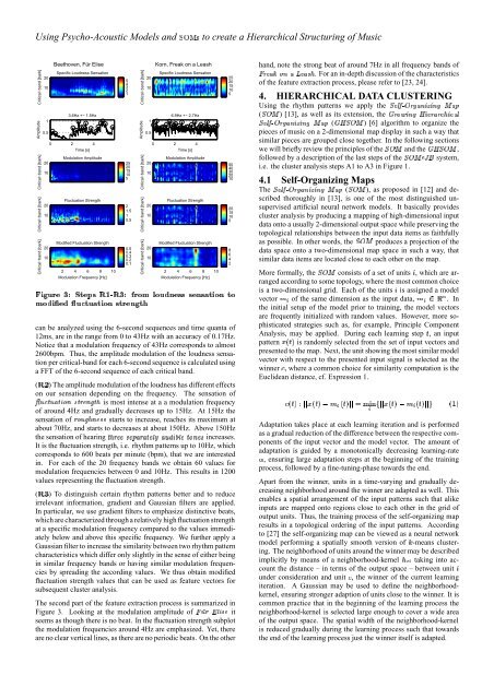
Beethoven, Für Elise<br />
Specific Loudness Sensation<br />
3.6Hz +− 1.5Hz<br />
0 2 4<br />
Time [s]<br />
Modulation Amplitude<br />
Fluctuation Strength<br />
Modified Fluctuation Strength<br />
2 4 6 8 10<br />
Modulation Frequency [Hz]<br />
¦4¦Ž4‘<br />
†ˆ‡y‰.Š5‹9Œ<br />
Œ"£BÉ0ŠF ’v˜4£O‡tÂ<br />
5<br />
4<br />
3<br />
2<br />
1<br />
25<br />
20<br />
15<br />
10<br />
5<br />
2<br />
1.5<br />
1<br />
0.5<br />
0.5<br />
0.4<br />
0.3<br />
0.2<br />
0.1<br />
Critical−b<strong>and</strong> [bark]<br />
Amplitude<br />
Critical−b<strong>and</strong> [bark]<br />
Critical−b<strong>and</strong> [bark]<br />
Critical−b<strong>and</strong> [bark]<br />
20<br />
10<br />
1<br />
0.5<br />
20<br />
10<br />
20<br />
10<br />
20<br />
10<br />
Korn, Freak on a Leash<br />
Specific Loudness Sensation<br />
6.9Hz +− 2.7Hz<br />
0 2 4<br />
Time [s]<br />
Modulation Amplitude<br />
Fluctuation Strength<br />
Modified Fluctuation Strength<br />
2 4 6 8 10<br />
Modulation Frequency [Hz]<br />
ž ‹9˜=’È¡y˜.Š5£ š5Œ j Œsš ¢‘<br />
‡y˜.š<br />
—OqǦ€œÇº¦4 ‡y˜=š<br />
‘<br />
‹Œ¢š4‰<br />
‘9¼ ¢‘<br />
can be analyzed using the 6-second sequences <strong>and</strong> time quanta of<br />
12ms, are in the range from 0 <strong>to</strong> 43Hz with an accuracy of 0.17Hz.<br />
Notice that a modulation frequency of 43Hz corresponds <strong>to</strong> almost<br />
2600bpm. Thus, the amplitude modulation of the loudness sensation<br />
per critical-b<strong>and</strong> for each 6-second sequence is calculated using<br />
a FFT of the 6-second sequence of each critical b<strong>and</strong>.<br />
) The amplitude modulation of the loudness has different effects<br />
(Ǻ„<br />
on our sensation depending on the frequency. The sensation of<br />
Ê [ $~ [ ~g®~ \ _:go~yh is most intense at a a modulation frequency<br />
of around 4Hz <strong>and</strong> gradually decreases up <strong>to</strong> 15Hz. At 15Hz the<br />
sensation of \ [ o9hg._: starts <strong>to</strong> increase, reaches its maximum at<br />
about 70Hz, <strong>and</strong> starts <strong>to</strong> decreases at about 150Hz. Above 150Hz<br />
the sensation of hearing ~yh \ __¤_7w" \ ~7_$© }º [ ik©t_|~*g._: increases.<br />
It is the fluctuation strength, i.e. rhythm patterns up <strong>to</strong> 10Hz, which<br />
corresponds <strong>to</strong> 600 beats per minute (bpm), that we are interested<br />
in. For each of the 20 frequency b<strong>and</strong>s we obtain 60 values for<br />
modulation frequencies between 0 <strong>and</strong> 10Hz. This results in 1200<br />
values representing the fluctuation strength.<br />
) To distinguish certain rhythm patterns better <strong>and</strong> <strong>to</strong> reduce<br />
(Ǻ¦<br />
irrelevant information, gradient <strong>and</strong> Gaussian filters are applied.<br />
In particular, we use gradient filters <strong>to</strong> emphasize distinctive beats,<br />
which are characterized through a relatively high fluctuation strength<br />
at a specific modulation frequency compared <strong>to</strong> the values immediately<br />
below <strong>and</strong> above this specific frequency. We further apply a<br />
Gaussian filter <strong>to</strong> increase the similarity between two rhythm pattern<br />
characteristics which differ only slightly in the sense of either being<br />
in similar frequency b<strong>and</strong>s or having similar modulation frequencies<br />
by spreading the according values. We thus obtain modified<br />
fluctuation strength values that can be used as feature vec<strong>to</strong>rs for<br />
subsequent cluster analysis.<br />
The second part of the feature extraction process is summarized in<br />
Figure 3. Looking at the modulation amplitude XZY [Q\º] © A$_ of it<br />
seems as though there is no beat. In the fluctuation strength subplot<br />
the modulation frequencies around 4Hz are emphasized. Yet, there<br />
are no clear vertical lines, as there are no periodic beats. On the other<br />
25<br />
20<br />
15<br />
10<br />
5<br />
50<br />
40<br />
30<br />
20<br />
10<br />
20<br />
15<br />
10<br />
5<br />
8<br />
6<br />
4<br />
2<br />
h<strong>and</strong>, note the strong beat of around 7Hz in all frequency b<strong>and</strong>s of<br />
X \ _C9ƒgqx¹F_C»h . For an in-depth discussion of the characteristics<br />
of the feature extraction process, please refer <strong>to</strong> [23, 24].<br />
4. HIERARCHICAL DATA CLUSTERING<br />
<strong>Using</strong> the rhythm patterns we apply the `=_$©r$ea \ oRgst$AgQo¸bvw<br />
) [13], as well as its extension, the m \ nAgQoqp¤_ \ \ hQ©<br />
(`5aNb<br />
\ oRgst$AgQovbv:w (mNp¤`5aNb ) [6] algorithm <strong>to</strong> organize the<br />
`=_$©r$ea<br />
pieces of music on a 2-dimensional map display in such a way that<br />
similar pieces are grouped close <strong>to</strong>gether. In the following sections<br />
we will briefly review the principles of `Fa0b the <strong>and</strong> mNp{`Fa0b the ,<br />
followed by a description of the last steps of `5aNbc_d the system,<br />
i.e. the cluster analysis steps A1 <strong>to</strong> A3 in Figure 1.<br />
4.1 <strong>Self</strong>-<strong>Organizing</strong> <strong>Maps</strong><br />
The `._$©r$ea \ oRg¢t$AgoËbv:w (`FaNb ), as proposed in [12] <strong>and</strong> described<br />
thoroughly in [13], is one of the most distinguished unsupervised<br />
artificial neural network models. It basically provides<br />
cluster analysis by producing a mapping of high-dimensional input<br />
data on<strong>to</strong> a usually 2-dimensional output space while preserving the<br />
<strong>to</strong>pological relationships between the input data items as faithfully<br />
as possible. In other words, `5aNb the produces a projection of the<br />
data space on<strong>to</strong> a two-dimensional map space in such a way, that<br />
similar data items are located close <strong>to</strong> each other on the map.<br />
More formally, the `FaNb<br />
consists of a set of units Ì , which are arranged<br />
according <strong>to</strong> some <strong>to</strong>pology, where the most common choice<br />
is a two-dimensional grid. Each of the units Ì is assigned a model<br />
vec<strong>to</strong>r ÍqÎ of the same dimension as the input data, ÍqÎ|ϸÐÑ . In<br />
the initial setup of the model prior <strong>to</strong> training, the model vec<strong>to</strong>rs<br />
are frequently initialized with r<strong>and</strong>om values. However, more sophisticated<br />
strategies such as, for example, Principle Component<br />
Analysis, may be applied. During each learning step Ò , an input<br />
pattern ÓOÔAÒÕ is r<strong>and</strong>omly selected from the set of input vec<strong>to</strong>rs <strong>and</strong><br />
presented <strong>to</strong> the map. Next, the unit showing the most similar model<br />
vec<strong>to</strong>r with respect <strong>to</strong> the presented input signal is selected as the<br />
winner Ö , where a common choice for similarity computation is the<br />
Euclidean distance, cf. Expression 1.<br />
θà ÙtÙÓOÔAÒCÕ ÚvÍjÎCÔAÒCÕÙtÙ á Ô»âÕ<br />
ÖÔAÒÕØ×'ÙtÙÓOÔAÒCÕFÚcÍuÛÔAÒCÕÙtÙÜÄ݃Þtß<br />
Adaptation takes place at each learning iteration <strong>and</strong> is performed<br />
as a gradual reduction of the difference between the respective components<br />
of the input vec<strong>to</strong>r <strong>and</strong> the model vec<strong>to</strong>r. The amount of<br />
adaptation is guided by a mono<strong>to</strong>nically decreasing<br />
ã<br />
learning-rate<br />
, ensuring large adaptation steps at the beginning of the training<br />
process, followed by a fine-tuning-phase <strong>to</strong>wards the end.<br />
Apart from the winner, units in a time-varying <strong>and</strong> gradually decreasing<br />
neighborhood around the winner are adapted as well. This<br />
enables a spatial arrangement of the input patterns such that alike<br />
inputs are mapped on<strong>to</strong> regions close <strong>to</strong> each other in the grid of<br />
output units. Thus, the training process of the self-organizing map<br />
results in a <strong>to</strong>pological ordering of the input patterns. According<br />
<strong>to</strong> [27] the self-organizing map can be viewed as a neural network<br />
model performing a spatially smooth version of ä -means clustering.<br />
The neighborhood of units around the winner may be described<br />
implicitly by means of a neighborhood-kernel å¢ÛLÎ taking in<strong>to</strong> account<br />
the distance – in terms of the output space – between unit Ì<br />
under consideration <strong>and</strong> Ö unit , the winner of the current learning<br />
iteration. A Gaussian may be used <strong>to</strong> define the neighborhoodkernel,<br />
ensuring stronger adaption of units close <strong>to</strong> the winner. It is<br />
common practice that in the beginning of the learning process the<br />
neighborhood-kernel is selected large enough <strong>to</strong> cover a wide area<br />
of the output space. The spatial width of the neighborhood-kernel<br />
is reduced gradually during the learning process such that <strong>to</strong>wards<br />
the end of the learning process just the winner itself is adapted.

![Informationsvisualisierung [WS0708 | 01 ]](https://img.yumpu.com/22537403/1/190x143/informationsvisualisierung-ws0708-01-.jpg?quality=85)