Using Psycho-Acoustic Models and Self-Organizing Maps to Create ...

W
Using Psycho-Acoustic Models and ¢¡¤£¦¥ to create a Hierarchical Structuring of Music
Using Psycho-Acoustic Models and Self-Organizing Maps
to Create a Hierarchical Structuring of
Music by Sound Similarity
§
Andreas Rauber
Dept. of Software Technology
Vienna Univ. of Technology
A-1040 Vienna, Austria
andi@ifs.tuwien.ac.at
ABSTRACT
With the advent of large musical archives the need to provide an
organization of these archives becomes eminent. While artist-based
organizations or title indexes may help in locating a specific piece
of music, a more intuitive, genre-based organization is required to
allow users to browse an archive and explore its contents. Yet,
currently these organizations following musical styles have to be
designed manually.
In this paper we propose an approach to automatically create a
hierarchical organization of music archives following their perceived
sound similarity. More specifically, characteristics of frequency
spectra are extracted and transformed according to psycho-acoustic
models. Subsequently, the Growing Hierarchical Self-Organizing
Map, a popular unsupervised neural network, is used to create a
hierarchical organization, offering both an interface for interactive
exploration as well as retrieval of music according to perceived
sound similarity.
1. INTRODUCTION
With the availability of high-quality audio file formats at sufficient
compression rates, we find music increasingly being distributed
electronically via large music archives, offering music from the
public domain, selling titles, or streaming them on a pay-per-play
basis, or simply in the form of on-line retailers for conventional
distribution channels. A core requirement for these archives is the
possibility for the user to locate a title he or she is looking for, or to
find out which types of music are available in general.
Thus, those archives commonly offer several ways to find a desired
piece of music. A straightforward approach is to use text based
queries to search for the artist, the title or some phrase in the lyrics.
While this approach allows the localization of a desired piece of music,
it requires the user to know and actively input information about
the title he or she is looking for. An alternative approach, allowing
users to explore the music archive, searching for musical styles,
rather than for a specific title or group, is thus usually provided in the
form of genre hierarchies such as ¨©© , , . Hence, a
customer looking for an opera recording might look into the ¨©
section, and will there find - depending on the further organization of
the music archive - a variety of interpretations, being similar in style,
and thus possibly suiting his or her likings. However, such organizations
rely on manual categorizations and usually consist of several
hundred categories which involve high maintenance costs, in particular
for dynamic music collections, where multiple contributors
"!$#%'&(%*)+ ,¢-.&$#/0-.!$,'1&$234-5)+ 6 3.%7)34!$89%7)&$#"-.!$,'!:2;=.?A@B

‘
‘
—
Using Psycho-Acoustic Models and ¢¡¤£¦¥ to create a Hierarchical Structuring of Music
available as MIDI. A more readily available format is the raw audio
signal to which all other audio formats can be decoded. One of the
first audio retrieval approaches dealing with music was presented
in [35], where attributes such as the pitch, loudness, brightness and
bandwidth of speech and individual musical notes were analyzed.
Several overviews of systems based on the raw audio data have been
presented, e.g. [9, 18]. However, most of these systems do not treat
content-based music retrieval in detail, but mainly focus on speech
or partly-speech audio data, with one of the few exceptions being
presented in [17], using hummed queries against an MP3 archive
for melody-based retrieval.
Furthermore, only few approaches in the area of content-based music
analysis have utilized the framework of psychoacoustics. Psychoacoustics
deals with the relationship of physical sounds and the human
brain’s interpretation of them, cf. [37]. One of the first exceptions
was [8], where psychoacoustic models are used to describe the similarity
of instrumental sounds. The approach was demonstrated using
a collection of about 100 instruments, which were organized using
a `._$©r$ea \ oRg¢t$Agojbv:w in a similar way as presented in this paper.
For each instrument a 300 milliseconds sound was analyzed and
steady state sounds with a duration of 6 milliseconds were extracted.
These steady state sounds can be regarded as the smallest possible
building blocks of music. A model of the human perceptual behavior
of music using psychoacoustic findings was presented in [30]
together with methods to compute the similarity of two pieces of
music. A more practical approach to the topic was presented in [33]
where music given as raw audio is classified into genres based on
musical surface and rhythm features. The features are similar to
the rhythm patterns we extract, the main difference being that we
analyze them separately in 20 frequency bands.
Our work is based on first experiments reported in [26]. In particular
we have redesigned the feature extraction process using psychoacoustic
models. Additionally, by using a hierarchical extension of
the neural network for data clustering we are able to detect the
hierarchical structure within our archive.
3. FEATURE EXTRACTION
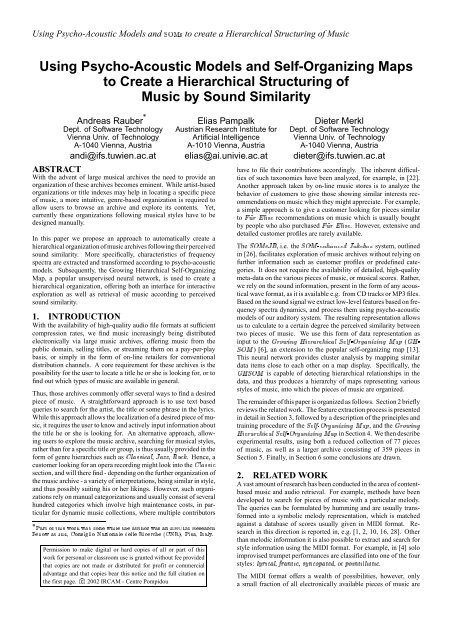
The architecture of the `Fa0bc_d system may be divided into 3
stages as depicted in Figure 1. Digitized music in good sound quality
(44kHz, stereo) with a duration of one minute is represented
by approximately 10MB of data in its raw format describing the
physical properties of the acoustical waves we hear. In a preprocessing
stage, the audio signal is transformed, down-sampled and
split into individual segments (steps P1 to P3). We then extract features
which are robust towards non-perceptive variations and on the
other hand resemble characteristics which are critical to our hearing
sensation, i.e. rhythm patterns in various frequency bands. The
feature extraction stage can be divided into two subsections, consisting
of the extraction of the specific loudness sensation expressed in
`'g._ (steps S1 to S6), as well as the conversion into time-invariant
frequency-specific rhythm patterns (step R1 to R3). Finally, the data
may be optionally converted, before being organized into clusters in
steps A1 to A3 using the mNp{`Fa0b . The feature extraction steps are
further detailed in the following subsections, with the clustering procedure
being described in Section 4, with the visualization metaphor
being only touched upon briefly due to space considerations.
3.1 Preprocessing
€ ) The pieces of music may be given in any audio file format,
(
such as e.g. MP3 files. We first decode these to the ‚ [ © $_ƒ¨0iR_
raw
[ ©~g (PCM) audio format.
bvi
) The raw audio format of music in good quality requires huge
(…„
amounts of storage. As humans can easily identify the genre of a
piece of music even if its sound quality is rather poor we can safely
reduce the quality of the audio signal. Thus, stereo sound quality
is first reduced to mono and the signal is then down-sampled from
F
e
a
t
u
r
e
E
x
t
r
a
c
t
i
o
n
Preprocessing
Specific
Loudness
Sensation
(Sone)
Rhythm
Patterns
per
Frequency
Band
Analysis
P1: Audio -> PCM
P2: Stereo -> Mono, 44kHz->11kHz
P3: music -> segments
S1: Power Spectrum
S2: Critical Bands
S3: Spectral Masking
S4:Decibel - dB-SPL
S5: Phon: Equal Loudness
S6: Sone: Specific Loudness Sens.
R1: Modulation Amplitude
R2: Fluctuation Strength
R3: Modified Fluctuation Strength
A1: Median vector (opt.)
A2: Dimension Reduction (opt.)
A3: GHSOM Clustering
Visualization: Islands of Music and Weather Charts
€¢fŽ45‘
Œs’”“ •=Œ"‹•F‡yŒQ–
q—
‹Œ ‹˜4Œ
‡š5‰F› „"œ‘ ‰'Œ
†ˆ‡y‰=ŠF‹Œ
Œ
¢‘
Š5‹9ŒqŒ"Ÿ ‹ ‡y˜.š0› R¡Š
‘
Œ"‹ š ¡
F ‡ ¢ šF£¤•5‡ Š ¡A‡y¥ s‘
ž
‡y˜.š
44kHz to 11kHz, leaving a distorted, but still easily recognizable
sound signal comparable to phone line quality.
) We subsequently segment each piece into 6-second sequences.
(…¦
The duration of 6 (§R¨L© seconds samples) was chosen heuristically
because it is long enough for humans to get an impression of the
style of a piece of music while being short enough to optimize
the computations. However, analyses with various settings for the
segmentation have shown no significant differences with respect to
segment length. After removing the first and the last 2 segments
of each piece of music to eliminate lead-in and fade-out effects,
we retain only every third of the remaining segments for further
analysis. Again, the information lost by this type of reduction has
shown insignificant in various experimental settings.
We thus end up with several segments of 6 seconds of music every
18 seconds at 11kHz for each piece of music. The preprocessing
results in a data reduction by a factor of over 24 without losing
relevant information, i.e. a human listener is still able to identify the
genre or style of a piece of music given the few 6-second sequences
in lower quality.
3.2 Specific Loudness Sensation - Sone
Loudness belongs to the category of intensity sensations. The loudness
of a sound is measured by comparing it to a reference sound.
The 1kHz tone is a very popular reference tone in psychoacoustics,

˜
‘
Œ
Œ
‘
¥
Using Psycho-Acoustic Models and ¢¡¤£¦¥ to create a Hierarchical Structuring of Music
and the loudness of the 1kHz tone at 40dB is defined to be ªZ`'g._ .
A sound perceived to be twice as loud is defined to be 2 `=g=_ and
so on. In the first stage of the feature extraction process, this specific
loudness sensation (Sone) per critical-band (Bark) in short time
intervals is calculated in 6 steps starting with the PCM data.
) First the power spectrum of the audio signal is calculated. To
(Ž€
do this, the raw audio data is first decomposed into its frequencies
using X4~NX5 [Q\ *_ \u«s\ gsSr \¬ ~g®­X X «'¯
a . We use a window
size of 256 samples, which corresponds to about 23ms at 11kHz,
and a Hanning window with 50% overlap. We thus obtain a Fourier
transform of 11 / 2 kHz, i.e. 5.5 kHz signals.
) The inner ear separates the frequencies and concentrates them
(ŽF„
at certain locations along the basilar membrane. The inner ear
can thus be regarded as a complex system of a series of bandpass
filters with an asymmetrical shape of frequency response. The
center frequencies of these band-pass filters are closely related to the
critical-band rates, where frequencies are bundled into 24 criticalbands
according to the d| \ scale [37]. Where these bands should
be centered, or how wide they should be, has been analyzed through
several psychoacoustic experiments. Since our signal is limited to
5.5 kHz we use only the first 20 critical bands, summing up the
values of the power spectrum within the upper and lower frequency
limits of each band, obtaining a power spectrum of the 20 critical
bands for the segments.
) Spectral Masking is the occlusion of a quiet sound by a louder
(ŽF¦
sound when both sounds are present simultaneously and have similar
frequencies. Spectral masking effects are calculated based on [31],
with a spreading function defining the influence of ° the -th critical
band on the -th being used to obtain a spreading matrix. Using
this matrix the power spectrum is spread across the critical bands
obtained in the previous step, where the masking influence of a
critical band is higher on bands above it than on those below it.
) The intensity unit of physical audio signals is sound pressure
(Ž4±
and is measured ‚:© in (Pa). The values of the PCM data
correspond to the sound pressure. Before `=g._ calculating values
it is necessary to transform the data into decibel. The decibel value
of a sound is calculated as the ratio between its pressure and the
pressure of the hearing threshold, also known as dB-SPL, where
SPL is the abbreviation for sound pressure level.
) The relationship between the sound pressure level in decibel
(ŽF²
and our hearing sensation measured `'g._ in is not linear. The
perceived loudness depends on the frequency of the tone. From the
dB-SPL values we thus calculate the equal loudness levels with their
unit Phon. The ‚Nhsg levels are defined through the loudness in dB-
SPL of a tone with 1kHz frequency. A level of 40 ‚0hsg resembles
the loudness level of a 40dB-SPL tone at 1kHz. A pure tone at
any frequency with 40 ‚0hsg is perceived as loud as a pure tone
with 40dB at 1kHz. We are most sensitive to frequencies around
2kHz to 5kHz. The hearing threshold rapidly rises around the lower
and upper frequency limits, which are respectively about 20Hz and
16kHz. Although the values for the equal loudness contour matrix
are obtained from experiments with pure tones, they may be applied
to calculate the specific loudness of the critical band rate spectrum,
resulting in loudness level representations for the frequency ranges.
) Finally, as the perceived loudness sensation differs for different
(ŽF³
loudness levels, the specific loudness sensation `=g=_ in is calculated
based on [3]. The loudness of the 1kHz tone at 40dB-SPL is defined
to be 1 Sone. A tone perceived twice as loud is defined to be `=g=_ 2
and so on. For values up to ‚0hsg 40 the sensation rises slowly,
increasing at a faster rate afterwards.
Figure 2 illustrates the data after each of the feature extraction steps
using the first 6-second sequences extracted from d{__:~yhs´_:g¢µNXZY [Q\
] © A$_ and from ^ \ g¢µ·X \ _fģ º¹F_C»h . The sequence of XZY
Amplitude
0.05
0
−0.05
Frequency [kHz]
Critical−band [bark]
Critical−band [bark]
Critical−band [bark]
Critical−band [bark]
4
2
PCM Audio Signal
Power Spectrum [dB]
0
Critical−Band Rate Spectrum [dB]
20
15
10
5
Spread Critical−Band Rate Spectrum [dB]
20
15
10
5
20
15
10
5
Specific Loudness Level [phon]
Specific Loudness Sensation [sone]
20
15
10
5
†ˆ‡y‰=ŠF‹Œ
¡ ‡S‰.š
Beethoven, Für Elise
0 2 4
Time [s]
60
40
20
60
40
20
60
40
20
60
40
20
5
4
3
2
1
Amplitude
Frequency [kHz]
Critical−band [bark]
Critical−band [bark]
Critical−band [bark]
Critical−band [bark]
1
0
−1
4
2
PCM Audio Signal
Power Spectrum [dB]
0
Critical−Band Rate Spectrum [dB]
20
15
10
5
Spread Critical−Band Rate Spectrum [dB]
20
15
10
5
20
15
10
5
Specific Loudness Level [phon]
Specific Loudness Sensation [sone]
20
15
10
5
Korn, Freak on a Leash
0 2 4
Time [s]
—OuŽ€Rœ:Ž5³4 ž ‹˜.’ ‘9¼ €'€Q½4¾ ¢¿^ÀÁ ŠF£F‡y˜
„4ZŽ4‘ Œs‡S¦¡y˜.Š5£ š5Œ
z—
Œs‹ZR‹9‡ ‡A ¡
œÃF š5£
—
© A$_ contains the main theme starting shortly before the 2nd second.
]
The specific loudness sensation depicts each piano key played. On
the other X \ _¤gÄj¹F_C»h hand, , which is classified p¢_C´} as
, is quite aggressive. Melodic elements do not
bv_:~*©Å"Æ^_C~yhubc_:~*©
play a major role and the specific loudness sensation is a rather
complex pattern spread over the whole frequency range, whereas
only the lower critical bands are active XZY [Q\] © A$_ in . Notice further,
that the values of the patterns X \ _C9vģ q¹F_C»h of are up to 18
times higher compared to those XZY [Q\{] © A$_ of .
3.3 Rhythm Patterns
After the first preprocessing stage a piece of music is represented
by several 6-second sequences. Each of these sequences contains
information on how loud the piece is at a specific point in time in a
specific frequency band. Yet, the current data representation is not
time-invariant. It may thus not be used to compare two pieces of
music point-wise, as already a small time-shift of a few milliseconds
will usually result in completely different feature vectors. In the
second stage of the feature extraction process, we calculate a timeinvariant
representation for each piece of music in 3 further steps,
namely the frequency-wise rhythm pattern. These rhythm patterns
contain information on how strong and fast beats are played within
the respective frequency bands.
) The loudness of a critical-band usually rises and falls several
(Çj€
times resulting in a more or less periodical pattern, also known as
the rhythm. The loudness values of a critical-band over a certain
time period can be regarded as a signal that has been sampled at
discrete points in time. The periodical patterns of this signal can
then be assumed to originate from a mixture of sinuids. These
sinuids modulate the amplitude of the loudness, and can be calculated
by a Fourier transform. The modulation frequencies, which
80
60
40
20
80
60
40
80
60
40
80
60
40
25
20
15
10
5
[Q\

Œ
Š
‘
˜
‘
Using Psycho-Acoustic Models and ¢¡¤£¦¥ to create a Hierarchical Structuring of Music
Critical−band [bark]
Amplitude
Critical−band [bark]
Critical−band [bark]
Critical−band [bark]
20
10
1
0.5
20
10
20
10
20
10
Beethoven, Für Elise
Specific Loudness Sensation
3.6Hz +− 1.5Hz
0 2 4
Time [s]
Modulation Amplitude
Fluctuation Strength
Modified Fluctuation Strength
2 4 6 8 10
Modulation Frequency [Hz]
¦4¦Ž4‘
†ˆ‡y‰.Š5‹9Œ
Œ"£BÉ0ŠF ’v˜4£O‡tÂ
5
4
3
2
1
25
20
15
10
5
2
1.5
1
0.5
0.5
0.4
0.3
0.2
0.1
Critical−band [bark]
Amplitude
Critical−band [bark]
Critical−band [bark]
Critical−band [bark]
20
10
1
0.5
20
10
20
10
20
10
Korn, Freak on a Leash
Specific Loudness Sensation
6.9Hz +− 2.7Hz
0 2 4
Time [s]
Modulation Amplitude
Fluctuation Strength
Modified Fluctuation Strength
2 4 6 8 10
Modulation Frequency [Hz]
ž ‹9˜=’È¡y˜.Š5£ š5Œ j Œsš ¢‘
‡y˜.š
—OqǦ€œÇº¦4 ‡y˜=š
‘
‹Œ¢š4‰
‘9¼ ¢‘
can be analyzed using the 6-second sequences and time quanta of
12ms, are in the range from 0 to 43Hz with an accuracy of 0.17Hz.
Notice that a modulation frequency of 43Hz corresponds to almost
2600bpm. Thus, the amplitude modulation of the loudness sensation
per critical-band for each 6-second sequence is calculated using
a FFT of the 6-second sequence of each critical band.
) The amplitude modulation of the loudness has different effects
(Ǻ„
on our sensation depending on the frequency. The sensation of
Ê [ $~ [ ~g®~ \ _:go~yh is most intense at a a modulation frequency
of around 4Hz and gradually decreases up to 15Hz. At 15Hz the
sensation of \ [ o9hg._: starts to increase, reaches its maximum at
about 70Hz, and starts to decreases at about 150Hz. Above 150Hz
the sensation of hearing ~yh \ __¤_7w" \ ~7_$© }º [ ik©t_|~*g._: increases.
It is the fluctuation strength, i.e. rhythm patterns up to 10Hz, which
corresponds to 600 beats per minute (bpm), that we are interested
in. For each of the 20 frequency bands we obtain 60 values for
modulation frequencies between 0 and 10Hz. This results in 1200
values representing the fluctuation strength.
) To distinguish certain rhythm patterns better and to reduce
(Ǻ¦
irrelevant information, gradient and Gaussian filters are applied.
In particular, we use gradient filters to emphasize distinctive beats,
which are characterized through a relatively high fluctuation strength
at a specific modulation frequency compared to the values immediately
below and above this specific frequency. We further apply a
Gaussian filter to increase the similarity between two rhythm pattern
characteristics which differ only slightly in the sense of either being
in similar frequency bands or having similar modulation frequencies
by spreading the according values. We thus obtain modified
fluctuation strength values that can be used as feature vectors for
subsequent cluster analysis.
The second part of the feature extraction process is summarized in
Figure 3. Looking at the modulation amplitude XZY [Q\º] © A$_ of it
seems as though there is no beat. In the fluctuation strength subplot
the modulation frequencies around 4Hz are emphasized. Yet, there
are no clear vertical lines, as there are no periodic beats. On the other
25
20
15
10
5
50
40
30
20
10
20
15
10
5
8
6
4
2
hand, note the strong beat of around 7Hz in all frequency bands of
X \ _C9ƒgqx¹F_C»h . For an in-depth discussion of the characteristics
of the feature extraction process, please refer to [23, 24].
4. HIERARCHICAL DATA CLUSTERING
Using the rhythm patterns we apply the `=_$©r$ea \ oRgst$AgQo¸bvw
) [13], as well as its extension, the m \ nAgQoqp¤_ \ \ hQ©
(`5aNb
\ oRgst$AgQovbv:w (mNp¤`5aNb ) [6] algorithm to organize the
`=_$©r$ea
pieces of music on a 2-dimensional map display in such a way that
similar pieces are grouped close together. In the following sections
we will briefly review the principles of `Fa0b the and mNp{`Fa0b the ,
followed by a description of the last steps of `5aNbc_d the system,
i.e. the cluster analysis steps A1 to A3 in Figure 1.
4.1 Self-Organizing Maps
The `._$©r$ea \ oRg¢t$AgoËbv:w (`FaNb ), as proposed in [12] and described
thoroughly in [13], is one of the most distinguished unsupervised
artificial neural network models. It basically provides
cluster analysis by producing a mapping of high-dimensional input
data onto a usually 2-dimensional output space while preserving the
topological relationships between the input data items as faithfully
as possible. In other words, `5aNb the produces a projection of the
data space onto a two-dimensional map space in such a way, that
similar data items are located close to each other on the map.
More formally, the `FaNb
consists of a set of units Ì , which are arranged
according to some topology, where the most common choice
is a two-dimensional grid. Each of the units Ì is assigned a model
vector ÍqÎ of the same dimension as the input data, ÍqÎ|ϸÐÑ . In
the initial setup of the model prior to training, the model vectors
are frequently initialized with random values. However, more sophisticated
strategies such as, for example, Principle Component
Analysis, may be applied. During each learning step Ò , an input
pattern ÓOÔAÒÕ is randomly selected from the set of input vectors and
presented to the map. Next, the unit showing the most similar model
vector with respect to the presented input signal is selected as the
winner Ö , where a common choice for similarity computation is the
Euclidean distance, cf. Expression 1.
θà ÙtÙÓOÔAÒCÕ ÚvÍjÎCÔAÒCÕÙtÙ á Ô»âÕ
ÖÔAÒÕØ×'ÙtÙÓOÔAÒCÕFÚcÍuÛÔAÒCÕÙtÙÜÄ݃Þtß
Adaptation takes place at each learning iteration and is performed
as a gradual reduction of the difference between the respective components
of the input vector and the model vector. The amount of
adaptation is guided by a monotonically decreasing
ã
learning-rate
, ensuring large adaptation steps at the beginning of the training
process, followed by a fine-tuning-phase towards the end.
Apart from the winner, units in a time-varying and gradually decreasing
neighborhood around the winner are adapted as well. This
enables a spatial arrangement of the input patterns such that alike
inputs are mapped onto regions close to each other in the grid of
output units. Thus, the training process of the self-organizing map
results in a topological ordering of the input patterns. According
to [27] the self-organizing map can be viewed as a neural network
model performing a spatially smooth version of ä -means clustering.
The neighborhood of units around the winner may be described
implicitly by means of a neighborhood-kernel å¢ÛLÎ taking into account
the distance – in terms of the output space – between unit Ì
under consideration and Ö unit , the winner of the current learning
iteration. A Gaussian may be used to define the neighborhoodkernel,
ensuring stronger adaption of units close to the winner. It is
common practice that in the beginning of the learning process the
neighborhood-kernel is selected large enough to cover a wide area
of the output space. The spatial width of the neighborhood-kernel
is reduced gradually during the learning process such that towards
the end of the learning process just the winner itself is adapted.

“
‘
‘
‡
‘
Using Psycho-Acoustic Models and ¢¡¤£¦¥ to create a Hierarchical Structuring of Music
layer 0
æ n
layer 1
x(t)
m(t) m(t+1) c
c
c
layer 2
Input Space
Output Space
layer 3
‡S˜.š
˜=‹ £
‹ ‡šF‡š4‰ ’v˜4£FŒ"¡Ø•=Œ"
†J‡S‰.ŠF‹Œ
Œ"
ŠF‹Œ
²4jñ¤ò¦ó·ôˆõö ‹9 ¼
'—F‘
†ˆ‡y‰.ŠF‹Œ
±F^Ž
In combining these principles of self-organizing map training, we
may write the learning rule as given in Expression (2), with ã representing
the time-varying learning-rate, å ÛLÎ representing the timevarying
neighborhood-kernel, Ó representing the currently presented
input pattern, and ÍqÎ denoting the model vector assigned to unit Ì .
A simple graphical representation of a self-organizing map’s architecture
and its learning process is provided in Figure 4. In this
Í Î ÔAÒ5éÄâ9ÕÜÄÍ Î ÔAÒÕ4é ã ÔAÒÕOêå ÛLÎ ÔAÒCÕ êRëÓOÔAÒÕOÚfÍ Î ÔAÒÕ7ì
figure the output space consists of a square of 36 units, depicted
as circles, forming a grid of íºî¦í units. One input vector ÓOÔAÒCÕ is
randomly chosen and mapped onto the grid of output units. The
winner Ö showing the highest activation is determined. Consider the
winner being the unit depicted as the black unit labeled in the figure.
The model vector of the winner, ÍqÛÔAÒÕ , is now moved towards
the current input vector. This movement is symbolized in the input
space in Figure 4. As a consequence of the adaptation, unit Ö will
produce an even higher activation with respect to the input pattern
Ó at the next learning iteration, Ò.éïâ , because the unit’s model vector,
ÍqÛ9ÔAÒFéðâÕ , is now nearer to the input pattern Ó in terms of the
input space. Apart from the winner, adaptation is performed with
neighboring units, too. Units that are subject to adaptation are depicted
as shaded units in the figure. The shading of the various units
corresponds to the amount of adaptation, and thus, to the spatial
width of the neighborhood-kernel. Generally, units in close vicinity
of the winner are adapted more strongly, and consequently, they are
depicted with a darker shade in the figure.
Being a decidedly stable and flexible model, `5aNb the has been employed
in a wide range of applications, ranging from financial data
analysis, via medical data analysis, to time series prediction, industrial
control, and many more [5, 13, 32]. It basically offers itself
to the organization and interactive exploration of high-dimensional
data spaces. One of its most prominent application areas is the organization
of large text archives [15, 19, 29], which, due to numerous
computational optimizations and shortcuts that are possible in this
NN model, scale up to millions of documents [11, 14].
However, due to its topological characteristics, the `FaNb
Ô*§Õ
not only
serves as the basis for interactive exploration, but may also be used as
an index structure to high-dimensional databases, facilitating scalable
proximity searches. Reports on a combination of `5aNbË and
R*-trees as an index to image databases have been reported, for
example, in [20, 21], whereas an index tree based on the `FaNb
is reported in [36]. Thus, `5aNb the combines and offers itself in
a convenient way both for interactive exploration, as well as for
the indexing and retrieval, of information represented in the form
of high-dimensional feature spaces, where exact matches are either
impossible due to the fuzzy nature of data representation or
the respective type of query, or at least computationally prohibitive,
making them particularly suitable for image or music databases.
4.2 The GHSOM
The key idea of the m \ n0ygQoxp{*_ \ \ hQ©`=_$©r$ea \ oRgst$AgQô bvw [6]
is to use a hierarchical structure of multiple layers, where each layer
consists of a number of `5aNbË independent . `Fa0b One is used at
the first layer of the hierarchy, representing the respective data in
more detail. For every unit in this map `FaNb a might be added to
the next layer of the hierarchy. This principle is repeated with the
third and any further layers of mNp{`FaNb the .
Since one of the shortcomings `FaNb of usage is its fixed network
architecture we rather use an incrementally growing version of the
. This relieves us from the burden of predefining the network’s
`5aNb
size which is rather determined during the unsupervised training
process. We start with a layer 0, which consists of only one single
unit. The weight vector of this unit is initialized as the average of
all input data. The training process basically starts with a small map
of, § îj§ say, units in layer 1, which is self-organized according to
the `Fa0b
standard training algorithm.
This training process is repeated for a fixed number ÷ of training
iterations. Ever after ÷ training iterations the unit with the largest
deviation between its weight vector and the input vectors represented
by this very unit is selected as the error unit. In between the error unit
and its most dissimilar neighbor in terms of the input space either a
new row or a new column of units is inserted. The weight vectors
of these new units are initialized as the average of their neighbors.
An obvious criterion to guide the training process is ø [ g¢~9e
the
\:\ \¢ù Î , calculated as the sum of the distances between the
~gï_
weight vector of a Ì unit and the input vectors mapped onto this unit.
It is used to evaluate the mapping quality of `5aNb a based on
¬
the
[ gs~t~g¤_ \:\ \ (b®û ]
) of all units in the map. A map
_Cgúø
grows until b¤û ]
its falls below a certain ü ¨
fraction of the Î of
the unit ù in the preceding layer of the hierarchy. Thus, the map now
Ì
represents the data of the higher layer Ì unit in more detail.
As outlined above the initial architecture of the mNp{`Fa0b
consists
of `FaNb one . This architecture is expanded by another layer in case
of dissimilar input data being mapped on a particular unit. These
units are identified by a rather high quantization error Î which is
above a threshold ù . This threshold basically indicates the desired
ü9ý
granularity level of data representation as a fraction of the initial
quantization error at layer 0. In such a case, a new map will be
added to the hierarchy and the input data mapped on the respective
higher layer unit are self-organized in this new map, which again
grows until b®û ]
its is reduced to a ü ¨
fraction of the respective
higher layer unit’s quantization error Î . Note that this does not
necessarily lead to a balanced hierarchy. The depth of the hierarchy
will rather reflect the diversity in input data distribution which should
be expected in real-world data collections. Depending on the desired
ù ü ¨
fraction b®û ]
of reduction we may end up with either a very deep
hierarchy with small maps, a flat structure with large maps, or – in
the extreme case – only one large map. The growth of the hierarchy
is terminated when no further units are available for expansion.
Àèç

’
K
Using Psycho-Acoustic Models and ¢¡¤£¦¥ to create a Hierarchical Structuring of Music
1
4
7
0.5
0
0.5
0
0.7
2
5
8
0.9
0
1.8
0
1.8
3
6
9
1.1
0
0.9
0
0.9
music. We have evaluated several alternatives using Gaussian mixture
models, fuzzy c-means, and k-means pursuing the assumption
that a piece of music contains significantly different rhythm patterns.
However, the median, despite being by far the simplest technique,
yielded comparable results to the more complex methods. Other
simple alternatives such as the the mean proved to be too vulnerable
with respect to outliers.
1
4
7
10
0
ÔþRÕØÿ¡ ¢
9.1
0.3
4.4
0.3
4.8
0.3
9.1
0.5
Ô'Õ
Median
0
0.7
0
£¥¤§¦©¨
ߧ § Þ
¥
2
5
8
11
¦ ß þ
4.6
0.3
4.5
0.3
4.2
0.3
4.4
0.2
¦
ߦþ þ
¥ ¤
3
6
9
Median
0
6.9
0.3
9
0.3
4.7
0.3
4.2
³4 ç ¼
Œ ‹
¼=5‘9¼ —F¢‘‘
Œs‹š ˜ ž "!©!$#&%('*)§!+-,/.10
†ˆ‡y‰.Š5‹9Œ
! š5£

“
À
‘
Using Psycho-Acoustic Models and ¢¡¤£¦¥ to create a Hierarchical Structuring of Music
bfmc−uprocking
themangotree
bfmc−instereo
bfmc−rocking
bfmc−skylimit
bongobong
cocojambo
limp−n2gether
macarena
rockdj
conga
mindfiels
lovsisintheair
eifel65−blue
fromnewyorktola
gowest
manicmonday
radio
supertrouper
sl−summertime
rhcp−californication
rhcp−world
sl−whatigot
bfmc−freestyler
sexbomb
torn
ga−doedel
ga−iwantit
ga−japan
nma−bigblue
limp−nobody
pr−broken
ga−nospeech
limp−pollution
korn−freak
pr−deadcell
pr−revenge
dancingqueen
firsttime
foreveryoung
frozen
californiadream
risingsun
unbreakmyheart
missathing
friend
yesterday−b
eternalflame
feeling
drummerboy
fatherandson
ironic
future
lovemetender
therose
beethoven
fuguedminor
vm−bach
vm−brahms
bigworld
addict
ga−lie
angels
newyork
sml−adia
americanpie
lovedwoman
revolution
memory
rainbow
threetimesalady
branden
air
avemaria
elise
kidscene
mond
†ˆ‡y‰.ŠF‹Œkj
˜ ž ’vŠ ‡yq˜=¡y¡yŒ"
mlu¾¦Ž
‡y˜.š
the same general trends of organization, thus alleviating the common
problem of cluster separation in hierarchical organizations.
Some interesting insights into the music collection which the m0pxe
map, organizing the collection into 9 major styles of music. The
bottom right represents mainly classical music, while the upper left
mainly represents a mixture of Hip Hop, Electro, and House by
d| ¬ r [ g"zb¤¨ ­Ckr ¬ ¯
. The upper-right, center-right, and uppercenter
represent mainly disco music such ˆuÆ¢ as ˆRkk$_ by
¬ x­ \ iL° ¯
, dJ© [ _ by ] n|_$©poPq­C_: n|_$©roPqe7k© [ _ ¯
, or X \ _:g
Lº©A©
bfRiRgsg=¦­ r \ 9_:g ¯
by . Please note, that the organization does not
follow clean “conceptual” genre styles, splitting by definition, e.g.
wspx:w and p… [ $_ , but rather reflects the overall sound similarity.
p{
Seven of these 9 first-level categories are further refined on the second
level. For example, the bottom right unit representing classical
music is divided into 4 further sub-categories. Of these 4 categories
the lower-right represents slow and peaceful music, mainly
piano pieces such XZY as
© A$_Ë­C_$© A$_ ¯
and bvg'i:h¢_:Ags$g=~7_
[Q\Z]
¬ g=i ¯
by d{__:~yhs´_:g , or X \ _ ¬ i_º¹ Y g'i_ \q[ g=i¦bc_:g¢:h¢_:g by
­
[Q¬ gsg ­i$_:g=_ ¯
. The upper-right represents, for example,
`'h
pieces sg=_::Ëbf_ by (vm), which, in this case, are more dynamic
interpretations of classical pieces played on the violin. In the
upper-left orchestral music is located such as the as the end credits
of the dJR…~*¢~yhs_X [ ~ [Q\ _
KtKtK
­ r [ ~ [Q\ _ ¯
film and the slow love
«
song
by d{_:~~7_JbËis©t_ \ ­7~yh¢_ \ $_ ¯
, exhibiting a more intensive
h¢_ˆ$_
sound sensation, whereas the lower right corner unit represents the
\ g=iR_:g=k [Q\ ov¨0g'_ \ ~ by d|Rhf­»k \ g'i_:g ¯
.
d
Generally speaking, we find the softer, more peaceful songs on this
second level map located in the lower half of the map, whereas the
more dynamic, intensive songs are located in the upper half. This
corresponds to the general organization of the map in the first layer,
where the unit representing Classic music is located in the lower right
corner, having more aggressive music as its upper and left neighbors.
This allows us, even on lower-level maps, to move across map
boundaries to find similar music on the neighboring map following
reveals are, for example, that the song X \ __:~}©t_ \
by dJ ¬ e
`5aNb
[ gQjb®¨ (center-left) is quite different then the other songs by
r
the same X \ __:~}©t_ \
group. was the groups biggest hit so far and,
unlike their other songs, has been appreciate by a broader audience.
Generally, the pieces of one group have similar sound characteristics
and thus are located within the same categories. This applies, for
example, to the songs m [ g'vu·ws_:¤­oR ¯
of ‚:w"…Rhj­Sw \7¯
and ,
which are located in the center of the 9 first-level categories together
with other aggressive rock songs. However, another exception is
u¹O*_ by m [ g' uØws_:u­oRe*© *_ ¯
, located in the lowerleft.
Listening to this piece reveals, that it is much slower than the
¹OA´Ago¦Aģ
other pieces of the group, and that this song matches very well to,
for û iRi$~ example, xw ¨Fhs:_ by .
5.2 A GHSOM of 359 pieces of music
In this section we present results from using the `5aNbc_d system
to structure a larger collection of 359 pieces of music. Due to space
constraints we cannot display or discuss the full hierarchy in detail.
We will thus pick a few examples to show the characteristics of the
resulting hierarchy, inviting the reader to explore and evaluate the
complete hierarchy via the project homepage.
The mNp{`Fa0b
resulting has grown to a size §ºîzy of units on the
top layer map. All 8 top-layer units were expanded onto a second
layer in the hierarchy, from which 25 units out of 64 units total
on this layer were further expanded into a third layer. None of
the branches required expansion into a fourth layer at the required
level-of-detail setting. An integrated view of the two top-layers of
the map is depicted in Figure 8. We will now take a closer look at

“
À
‘
Using Psycho-Acoustic Models and ¢¡¤£¦¥ to create a Hierarchical Structuring of Music
†J‡S‰.ŠF‹Œ1{
‡y˜.š}|
˜ ž
ŒË¡ ‹‰'Œ"‹u’vŠ ‡Aj˜=¡y¡yŒ"
‡yŒ"Œ
mlu¾ËŽ
¦¢²(~c—
some branches of this map, and compare them to the respective areas
in the mNp{`FaNb of the smaller data collection depicted in Figure 7
Generally, we find pieces of soft classical music in the upper right
corner, with the music becoming gradually more dynamic and aggressive
as we move towards the bottom left corner of the map.
Due to the characteristics of the training process of the mNp{`FaNb
we can find the same general tendency at the respective lower-layer
maps. The overall orientation of the map hierarchy is rotated when
compared to the smaller mNp{`FaNb , where the classical titles were
located in the bottom right corner, with the more aggressive titles
placed on the upper left area of the map. This rotation is due to
the unsupervised nature of mNp¤`5aNb the training process. It can,
however, be avoided by using specific initialization techniques if a
specific orientation of the map were required.
The unit in the upper right corner of the top-layer map, representing
the softest classical pieces of music, is expanded onto a FZîj§ map
in the second layer (expanded to the upper right in Figure 8). Here
we again find the softest, most peaceful pieces in the upper right
corner, namely part of the sound-track of the movie [Q\ {‚ \ ,
next to ¹F_C´AgQou‚ \ ~ by ¬ _:¢px \ g._ \
,
« h¢_^bc_ \:\ }u‚ˆ_C:g¢~
by `'h [Q¬ gsg , and ¨0g=g by ‚Rh¢_$©k_$© . Below this unit we find
further soft titles, yet somewhat more dynamic. We basically find
all titles that were mapped together in the bottom right corner unit
of the smaller collection depicted in Figure 7 on
of mNp¤`5aNb the
this unit, uJ \ µ-uJ´_…bv \ µNXZY [Q\x] © A$_:µX \ _ ¬ i_¢¹ Y g'i_ \ [ g=i
i.e.
­i:_:g._ ¯
and the bvg'i:h¢_:Ag¢:g'~7_ . Furthermore,
bc_:gs:h¢_:ģ
a few additional titles of the larger collection have been mapped
onto this unit, the most famous of which probably Æx*_¢©t_:Ag=_
€
are
¬^[ S by bv \ ~ , the X [ g._ \ ©0bv \ h by ¨Fhs:w'yg or the
RhQ~
iRo from the Clarinet Concert by emphMozart.
û
Let us now take a look at the titles that were mapped onto the
neighboring units in the previously presented smaller data collection.
The d \ g'i_:g=k [Q\ oA:h¢_x^g9_ \ ~7_ , located on the neighboring unit
to the right in the first example, can be found in the lower left corner
of this map, together with, for u|© :zw \ RhzO \ ~yh [ ~ \
example,
hs \ i^`¢~ \ [ƒ‚
by . Mapped onto the upper neighboring unit in the
mNp{`FaNb smaller we had titles like X0 \ ~=bv´_ ¬ _:gs~OLrN~yh¢_q~yh
the
¬ wshsgs} by d{__:~yhs´_:g , or the « ~*ug'i¢X [ o_xyguÆ bËyg= \
`s}
d|h by . We find these two titles in the upper left corner of the
2-layer map of mNp¤`5aNb this , together with two of the three titles
mapped onto the diagonally neighboring unit in the mNp{`Fa0b first ,
¹4´_ ¬ _ « _:g'i_ \
i.e. by © ´A{‚ \ _:©t_:} , and « h¢_…ˆ_ by d{_:~~7_
]
\
, which are again soft, mellow, but a bit more dynamic. The
b¦is©t_
third title mapped onto this unit in the m0p¤`5aNb smaller , i.e. the
sound track of the d|j~*j~yh¢_^X [ ~ [Q\ _
movie is not mapped
into this branch of this mNp{`Fa0b
anymore. When we listen to this
title we find it to have mainly strong orchestral parts, which have a
different, more intense sound than the soft pieces mapped onto this
branch, which is more specific with respect to very soft classical titles
as more of them are available in the larger data collection. Instead,
we can find this title on the upper right corner in the neighboring
branch to the left, originating from the upper left corner unit of the
top-layer map. There it is mapped together with « h¢_…d|_ [ ~}qg'i
to be more or
less identical to the overall organization of the mNp{`FaNb
smaller in
so far as the titles present in both collections are mapped in similar
relative positions to each other.
and other orchestral pieces, such as u|©A©t_o \ ubv© ~* by
~yhs_ƒd{_C~
\ 9h ¬ . We thus find this branch of the mNp¤`5aNb
d
Due to the topology preservation provided by mNp{`FaNb the we can
move from the soft classical cluster map to the left to find somewhat
more dynamic classical pieces of music on the neighboring map
(expanded to the left in Figure 8). Thus, a typical disadvantage of
hierarchical clustering and structuring of datasets, namely the fact
that a cluster that might be considered conceptually very similar is
subdivided into two distinct branches, is alleviated in mNp{`Fa0b the
concept, because these data points are typically located in the close
neighborhood. We thus find, on the right border of the neighboring
map, the more peaceful titles of this branch, yet more dynamic than
the classical pieces on the neighboring right branch discussed above.
KtKtK
‘¼

K
­
K
€
K
€
K
K
K
K
Using Psycho-Acoustic Models and ¢¡¤£¦¥ to create a Hierarchical Structuring of Music
Rather than continuing to discuss the individual units we shall now
take a look at the titles of a specific artist and its distribution in
this hierarchy. In total, there are 7 titles s¢g._::¸bv_ by in
this collection, all violin interpretations, yet of distinctly different
style. Her most “conventional” classical interpretations, such as
`'h¢_ \ vyg ¨ðbËAg= \ ­7´ ¬ eLk \ 9h ¬ ¯
Brahm’s or ‚ \ ~y~*
„v…
Bach’s
] r \ `'©†s5© AgB­7´ ¬ e7kh ¯
are located in the classiccluster
in the upper right corner branch on two neighboring units
Ag
on the left side of the second-layer map. These are definitely the
most “classical” of her interpretations in the given collection, yet
exhibiting strong dynamics. Further 3 pieces of Vanessa Mae ( hs_
‡
« by Vivaldi, ˆ_Ci

€
€
K
€
K
K
K
€
K
K
€
K
K
K
K
€
K
K
K
€
K
K
€
K
K
K
K
K
€
K
K
K
€
€
€
K
€
€
K
€
Using Psycho-Acoustic Models and ¢¡¤£¦¥ to create a Hierarchical Structuring of Music
[7] M. Dittenbach, A. Rauber, and D. Merkl. Recent advances
with the growing hierarchical self-organizing map. In ‚ \
\ »hs:wBg¤`._$©r$ea \ oRg¢t$Agojbvw' , Advances in
»rƒ~yh¢_‘Lq
Self-Organizing Maps, pages 140–145, Lincoln, England, June
13-15 2001. Springer.
[8] B. Feiten and S. Günzel. Automatic indexing of a sound
database using self-organizing neural nets. ¨0 ¬ w [ ~7_ \ b [ e
[Q\ g=© , 18(3):53–65, 1994.
[9] J. Foote. An overview of audio information retrieval. b [ © ~e
¬ _Ciz`¢}~7_ ¬ , 7(1):2–10, 1999.
[10] A. Ghias, J. Logan, D. Chamberlin, and S. B.C. Query by
humming: Musical information retrieval in an audio database.
In ‚ \ {»rØ~yh¢_u¢¨Fb
236, San Francisco, CA, November 5 - 9 1995. ACM.
[11] S. Kaski. Fast winner search for SOM-based monitoring and
g¢~©w©=¨0grgƒb [ © ~ ¬ _Ci , pages 231–
retrieval of high-dimensional data. ‚ \ ^Lr{~yh¢_
In
\ ~ HØ$© _ [Q\ © _:~nN \ Ë­
g’u
945. IEE, September, 7.-10. 1999.
Ÿu
€Š€
gs~©w©O¨0gr
‰P‰ ¯
, pages 940–
[12] T. Kohonen. Self-organized formation of topologically correct
feature maps. dˆ©o©¨ }k:_ \ g._:~$ , 43:59–69, 1982.
[13] T. Kohonen. `._$©r$e7 \ oRg¢t$Ago ¬ :w' . Springer-Verlag, Berlin,
1995.
[14] T. Kohonen. Self-organization of very large document collections:
State of the art. ‚ \ {»rØ~yhs_ g¢~©w©.¨0grˆgu \ ~ HØ$©
In
[Q\ © _:~nN \ , pages 65–74, Skövde, Sweden, 1998.
_
[15] T. Kohonen, S. Kaski, K. Lagus, J. Salojärvi, J. Honkela,
V. Paatero, and A. Saarela. Self-organization of a massive document
collection.
]0]N] «s\ g¢:R$~g¢ˆg
11(3):574–585, May 2000.
K
[16] N. Kosugi, Y. Nishihara, T. Sakata, M. Yamamuro, and
K. Kushima. A practical query-by-humming system for a large
_ [Q\ ©
_:~nN \ ,
music database. ‚ \ »r¤~yh¢_“u¢¨Fb g¢~©w©0¨0gr…gqb [ © ~e
¬
In
, pages 333–342, Marina del Ray, CA, 2000. ACM.
_Ci
[23] E. Pampalk ©g=iv»rqb [ S$—’uJg=© }Aµ¦a \ oRgst~gsµ
K [ © 9~g¤Lrxb [ vu \ hQA´_: . Master’s thesis, Vienna
University of Technology,
g'i’s5y
2001.
[24] E. Pampalk, A. Rauber, and D. Merkl. Content-based organization
and visualization of music archives. In ‚ \ Z»rvu¢¨Fb
[ © ~ ¬ _i‹*Œ$Œ©‹ , Juan-les-Pins, France, December 1-6 2002.
b
ACM.
[25] E. Pampalk, A. Rauber, and D. Merkl. Using smoothed data
histograms for cluster visualization in self-organizing maps.
‚ uLr^~yh¢_ g¢~©w©¨0grƒg _ ["\ © _:~nN \ º­
€€
Ÿu
In
\
, Madrid, Spain, August 27-30 2002. Springer.
‹*Œ$Œ©‹ ¯
[26] A. Rauber and M. Frühwirth. Automatically analyzing and
organizing music ‚ \ ¦LrZ~yh¢_ ]·[Q\ ws_g ¨0gr
archives. In
\ h g=i1uJi´g=_Ci « _ChQg'©o}ºr \ Æxtoy~*©Ø¹ e
gBˆ_:$_
\ \ *_:x­ ] ¨FÆ|¹i‹*ŒPŒª ¯
, Darmstadt, Germany, Sept. 4-8 2001.
k
Springer.
[27] B. Ripley. ‚~~7_ \ g ˆ_ogsA~g g'i
Cambridge University Press, Cambridge, UK, 1996.
_ ["\ ©
_:~nN \ .
[28] J. Rolland, G. Raskinis, and J. Ganascia. Musical contentbased
retrieval: An overview of the Melodiscov approach and
system. In ‚ \ j»rz~yh¢_"u¢¨Fb
pages 81–84, Orlando, FL, 1999. ACM.
gs~©w©|¨0grºg®b [ © ~ ¬ _Ci ,
[29] D. Roussinov and H. Chen. Information navigation on the web
by clustering and summarizing query results. K gr$ \:¬ ~g
‚ \ _:ygQojg'iƒbvg=o_ ¬ _:g¢~ , 37:789 – 816, 2001.
[30] E. Scheirer. b [ eA¹ y~7_:gsAgQo^`s}~7_ ¬ . PhD thesis, MIT Media
Laboratory, 2000.
[31] M. Schröder, B. Atal, and J. Hall. Optimizing digital speech
coders by exploiting masking properties of the human ear.
[Q\ g=©Ø»r ~yh¢_Žû [ ~©N`=$_:~}Ë»rmu ¬ _ \ , 66:1647–
1652, 1979.
[17] C. Liu and P. Tsai. Content-based retrieval of mp3 music
objects. ‚ \ úLrË~yh¢_ g¢~©w©¢¨0grfg
In
¬ _:gs~|­:¨
…g=nˆ©t_io_xbvg'o_
Atlanta, Georgia, 2001. ACM.
gr \:¬ ~g g=i
¤b”‹aŒ$Œª ¯
, pages 506 – 511,
[18] M. Liu and C. Wan. A study of content-based classification and
retrieval of audio database. ‚ \ J»r0~yh¢_ gs~©w©Æ¢~*k_ ] g'e
In
\ AgQoËg'i•uØwRw=© ~g¢^`¢} ¬ w" [Q¬ ­ Æ ] u{`–‹*Œ$Œª ¯
,
oAg.__
Grenoble, France, 2001. IEEE.
[19] D. Merkl and A. Rauber. Document classification with unsupervised
neural networks. In F. Crestani and G. Pasi, editors,
Physica Verlag, 2000.
`=»r~N¨0 ¬ w [ ~AgQoxAg
gr \¬ ~g J_:~ \ *_:´© , pages 102–121.
[20] K. Oh, Y. Feng, K. Kaneko, A. Makinouchi, and S. Bae. SOMbased
R*-tree for similarity retrieval. ‚ \ c»rj~yh¢_ g¢~©w©
In
¬ {r$ \ uJi´g'_izu·wRw'© ~gs ,
¨0grºg¤Æ¢~*k_u`s}~7_
pages 182–189, Hong-Kong, China, April 18-21 2001. IEEE.
[21] K. Oh, K. Kaneko, and A. Makinouchi. Image classification
and retrieval based on wavelet-som. In K gs~©w©=`¢} ¬ w" [Q¬
u·ww=© ~gs Ag g¢e «"\ Riy~g=© ] g¢´ \ g'e
¬
gcÆ¢~*Rk$_ € «4] w ‰$‰ ¯
, pages 164–167, Kyoto, Japan, November
28-30 1999.
_:gs~x­Æu
IEEE.
[22] F. Pachet and D. Cazaly. A taxonomy of musical genres. In
‚ \ ¤»r~yh¢_
[ © ~ ¬ _Ci
gs~©w©4¨0grJg˨0g¢~7_:gs~ed|_Ci¢b
¯
, Paris, France, 2000.
u¢aC‹*Œ$Œ$Œ
g'e
[32] O. Simula, P. Vasara, J. Vesanto, and R. Helminen. The selforganizing
map in industry analysis. In L. Jain and V. Vemuri,
editors, g=i [ ~ \ ©auØwRw=© ~g¢ˆLr
Washington, DC., 1999. CRC Press.
K
_ [Q\ ©
_:~nN \ ,
[33] G. Tzanetakis, G. Essl, and P. Cook. Automatic musical genre
classification of audio signals. ‚ \ In
[ gr \:¬ ~gvˆ_:~ \ *_:´©Ø­ `"b
b
¬ w" [Q¬ g gs~©w©5`s}
¯
, Bloomington, In-
diana, October 15-17 2001.
[34] A. Ultsch and H. Siemon. Kohonen’s self-organizing feature
maps for exploratory data analysis. In ‚ \ …»r|~yh¢_
Netherlands, 1990. Kluwer.
\ ©
_:~nN \ ú¨0grº­
Kt€Š€
gs~©w©
_ [ e
¨vw ‰dŒ ¯
, pages 305–308, Dordrecht,
[35] E. Wold, T. Blum, D. Keislar, and J. Wheaton. Content-based
classification search and retrieval of audio. K ]0]N] b [ © ~ ¬ _$e
i , 3(3):27–36, Fall 1996.
[36] H. Zhang and D. Zhong. A scheme for visual feature based
image indexing. ‚ \ ¢LrJ~yh¢_ `˜ « Å¢`"‚
K ] ¨0gr{gq`s~* \ e
In
\ *_:´©9r$ \ K ¬ o_¤g'i1s5i_C…Æ¢~*k_: , pages
o_xg'i…J_:~
36–46, San Jose, CA, February 4-10 1995.
[37] E. Zwicker and H. ‚·}hsR [ ~$µNX5R$~xg=i bvie
Fastl.
, volume 22 of `._ \ *_:J»r gr \¬ ~gZ`=$*_:g'_: . Springer,
_$©
Berlin, 2. edition, 1999.
r \¬ ~g uJ_: ­