A Time-Dependent Enhanced Support Vector Machine For Time ...

where J i(t) = 0, for t < t i,J i(t) = 1, for t ≥ t i, t i being
the point in time the i-th level shift is detected. Even for
low values of j this model is likely to become complex and
difficult to interpret.
Instead, the intuition behind our approach will be to
change the loss function used in SVM regression, to place
special emphasis on distribution shift samples and their immediate
successors. The distribution shift is not treated as
an outlier, but instead, as useful information that we can incorporate
into an enhanced SVM regression algorithm. Details
are described next.
3.3 SVM Regression time-dependent empirical
loss
Let usconsider theclass of machinelearning methodsthat
address the learning process as finding the minimum of the
regularized risk function. Given n training samples (x i,y i)
(i=1,..., n), x i ∈ R d is the feature vector of the i–th training
sample, d is number of features, and y i ∈ R is the value we
are trying to predict, the regularized risk function will have
the form of:
L(w ∗ ) = argmin w φw T w+R emp(w) (2)
with w as the weight vector, φ is a positive parameter that
determines the influence
∑
of the structural error in Equation
2, and R emp(w) = 1 n
n i=1l(xi,yi,w) is the loss function
with l(x i,y i,w) as a measure of the distance between a true
label y i and the predicted label from the forecasting done
using w. The goal is now to minimize the loss function
L(w ∗ ), and for SupportVector Regression, this has the form
of
L(w ∗ ) = 1 n∑
2 || w ||2 +C (ξ + i +ξ − i ) (3)
subject to
i=1
{ 〈w,xi〉+b+ǫ+ξ + ≥ y i
〈w,x i〉+b−ǫ−ξ − ≤ y i
(4)
with b being the bias term, ξ + i
and ξ − i
as slack variables
to tolerate infeasible constraints in the optimization problem(for
soft margin SVM), C is a constant that determines
the trade-off between the slack variable penalty and the size
of the margin, and ǫ being the tolerated level of error.
The SupportVector Regression empirical loss for asample
x i with output y i is l 1(x i,y i,w)=max(0, |w T x i–y i|–ǫ), as
shown in Table 2. Each sample contribution to the loss is
independentfromtheothersamplescontribution, andallthe
samples are considered to be of same importance in terms
of information they possess.
The learning framework we aim to develop should be capable
of reducing the difference in error at selected samples.
The samples we focus on are samples where a distribution
shift is detected, as these samples are expected to be largeerror-producing
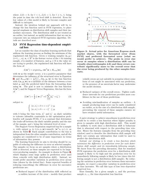
samples. An example is shown in Figure 3,
which displays some large spikes in prediction error (and
these coincide with high distribution shift). Instead, we
would prefer smoother variation in prediction error across
time (shown by the dotted line). Some expected benefits of
reducing (smoothing) the difference in error for successive
predictions are:
• Reduced impact of the distribution shift reflected as
a sudden increase of the error - models that produce
Figure 3: Actual price for American Express stock
market shares, with the forecasted error (from
SVM) and preferred forecasted error (what we
would prefer to achieve). The peaks in error size
occur at samples where a distribution shift can be
visually observed(samples 4-6) and these errors contribute
significantly more to the overall error that
the error being produced by the other samples forecasts.
volatile errors are not suitable in scenarios where some
form of cost might be associated with our prediction,
or the presence of an uncertain factor may undermine
the model decision.
• Reduced variance of the overall errors - Tighter confidence
intervals for our predictions provides more confidence
in the use of those predictions.
• Avoiding misclassification of samples as outliers - A
sample producing large error can be easily considered
an outlier, so in the case of a distribution shift sample,
preventing the removal of these samples ensures we
have retained useful information.
A naive strategy to achieve smoothness in prediction error
would be to create a loss function where higher penalty is
given to samples with high distribution shift. This would
be unlikely to work since a distribution shift is behaviour
that is abnormal with respect to the preceding time window.
Hence the features (samples from the preceding time
window) used to describe the distribution shift sample will
likely not contain any information that could be used to
predict the distribution shift.
Instead, our strategy is to create a loss function which
minimises the difference in prediction error for each distribution
shift sample and its immediately following sample.
We know from the preceding discussion, that for standard
SVM regression the prediction error for a distribution shift
sample is likely to be high and the prediction error for its
immediately following sample is likely be low (since this following
sample is not a distribution shift sample). By reducingthe
variation in predictionerror between these successive
samples, we expect a smoother variation in prediction error
as time increases. We call this type of loss time-dependent
empirical loss.
More formally, for a given sample x i and the previous
sample x i−1, the time-dependent loss function