arXiv:hep-th/9304011 v1 Apr 5 1993

YCTP-P23-92
LA-UR-92-3479
hep-th/9304011
arXiv:hep-th/9304011 v1 Apr 5 1993
P. Ginsparg
ginsparg@xxx.lanl.gov
MS-B285
Los Alamos National Laboratory
Los Alamos, NM 87545
Lectures on 2D Gravity
and
2D String Theory
and
Gregory Moore
moore@castalia.physics.yale.edu
Dept. of Physics
Yale University
New Haven, CT 06511
These notes are based on lectures delivered at the 1992 Tasi summer school. They constitute
the preliminary version of a book which will include many corrections and much more
useful information. Constructive comments are welcome.
Lectures given June 11–19, 1992 at TASI summer school, Boulder, CO
1992/1993

Contents
0. Introduction, Overview, and Purpose . . . . . . . . . . . . . . . . . . . . . . . 3
0.1. Philosophy and Diatribe . . . . . . . . . . . . . . . . . . . . . . . . . . 3
0.2. 2D Gravity and 2D String theory . . . . . . . . . . . . . . . . . . . . . . . 5
0.3. Review of reviews . . . . . . . . . . . . . . . . . . . . . . . . . . . . . 7
1. Loops and States in Conformal Field Theory . . . . . . . . . . . . . . . . . . . 8
1.1. Lagrangian formalism . . . . . . . . . . . . . . . . . . . . . . . . . . . . 8
1.2. Hamiltonian formalism . . . . . . . . . . . . . . . . . . . . . . . . . . . 9
1.3. Equivalence of states and operators . . . . . . . . . . . . . . . . . . . . . . 10
1.4. Gaussian Field with a Background Charge . . . . . . . . . . . . . . . . . . . 12
2. 2D Euclidean Quantum Gravity I: Path Integral Approach . . . . . . . . . . . . . 13
2.1. 2D Gravity and Liouville Theory . . . . . . . . . . . . . . . . . . . . . . . 13
2.2. Path integral approach to 2D Euclidean Quantum Gravity . . . . . . . . . . . . 14
3. Brief Review of the Liouville Theory . . . . . . . . . . . . . . . . . . . . . . . 22
3.1. Classical Liouville Theory . . . . . . . . . . . . . . . . . . . . . . . . . . 22
3.2. Classical Uniformization . . . . . . . . . . . . . . . . . . . . . . . . . . 24
3.3. Quantum Liouville Theory . . . . . . . . . . . . . . . . . . . . . . . . . 26
3.4. Spectrum of Liouville Theory . . . . . . . . . . . . . . . . . . . . . . . . 28
3.5. Semiclassical States . . . . . . . . . . . . . . . . . . . . . . . . . . . . . 31
3.6. Seiberg bound . . . . . . . . . . . . . . . . . . . . . . . . . . . . . . . 33
3.7. Semiclassical Amplitudes . . . . . . . . . . . . . . . . . . . . . . . . . . 35
3.8. Operator Products in Liouville Theory . . . . . . . . . . . . . . . . . . . . 39
3.9. Liouville Correlators from Analytic Continuation . . . . . . . . . . . . . . . . 40
3.10. Quantum Uniformization . . . . . . . . . . . . . . . . . . . . . . . . . . 41
3.11. Surfaces with boundaries . . . . . . . . . . . . . . . . . . . . . . . . . . 48
4. 2D Euclidean Quantum Gravity II: Canonical Approach . . . . . . . . . . . . . . 50
4.1. Canonical Quantization of Gravitational Theories . . . . . . . . . . . . . . . 50
4.2. Canonical Quantization of 2D Euclidean Quantum Gravity . . . . . . . . . . . 51
4.3. KPZ states in 2D Quantum Gravity . . . . . . . . . . . . . . . . . . . . . 52
4.4. LZ states in 2D Quantum Gravity . . . . . . . . . . . . . . . . . . . . . . 53
4.5. States in 2D Gravity Coupled to a Gaussian Field: more BRST . . . . . . . . . 54
5. 2D Critical String Theory . . . . . . . . . . . . . . . . . . . . . . . . . . . . 61
5.1. Particles in D Dimensions: QFT as 1D Euclidean Quantum Gravity. . . . . . . . 62
5.2. Strings in D Dimensions: String Theory as 2D Euclidean Quantum Gravity . . . . 64
5.3. 2D String Theory: Euclidean Signature . . . . . . . . . . . . . . . . . . . . 66
5.4. 2D String Theory: Minkowskian Signature . . . . . . . . . . . . . . . . . . . 68
5.5. Heterodox remarks regarding the “special states” . . . . . . . . . . . . . . . . 69
5.6. Bosonic String Amplitudes and the “c > 1 problem” . . . . . . . . . . . . . . 72
6. Discretized surfaces, matrix models, and the continuum limit . . . . . . . . . . . . 75
6.1. Discretized surfaces . . . . . . . . . . . . . . . . . . . . . . . . . . . . . 75
6.2. Matrix models . . . . . . . . . . . . . . . . . . . . . . . . . . . . . . . 77
6.3. The continuum limit . . . . . . . . . . . . . . . . . . . . . . . . . . . . 81
6.4. A first look at the double scaling limit . . . . . . . . . . . . . . . . . . . . 83
7. Matrix Model Technology I: Method of Orthogonal Polynomials . . . . . . . . . . . 84
1

7.1. Orthogonal polynomials . . . . . . . . . . . . . . . . . . . . . . . . . . . 84
7.2. The genus zero partition function . . . . . . . . . . . . . . . . . . . . . . 86
7.3. The all genus partition function . . . . . . . . . . . . . . . . . . . . . . . 88
7.4. The Douglas Equations and the KdV hierarchy . . . . . . . . . . . . . . . . 90
7.5. Ising Model . . . . . . . . . . . . . . . . . . . . . . . . . . . . . . . . 92
7.6. Multi-Matrix Models . . . . . . . . . . . . . . . . . . . . . . . . . . . . 94
7.7. Continuum Solution of the Matrix Chains . . . . . . . . . . . . . . . . . . . 95
8. Matrix Model Technology II: Loops on the Lattice . . . . . . . . . . . . . . . . . 99
8.1. Lattice Loop Operators . . . . . . . . . . . . . . . . . . . . . . . . . . . 99
8.2. Precise definition of the continuum limit . . . . . . . . . . . . . . . . . . 101
8.3. The Loop Equations . . . . . . . . . . . . . . . . . . . . . . . . . . . 103
9. Matrix Model Technology III: Free Fermions from the Lattice . . . . . . . . . . . 105
9.1. Lattice Fermi Field Theory . . . . . . . . . . . . . . . . . . . . . . . . 105
9.2. Eigenvalue distributions . . . . . . . . . . . . . . . . . . . . . . . . . . 106
9.3. Double–Scaled Fermi Theory . . . . . . . . . . . . . . . . . . . . . . . 109
10. Loops and States in Matrix Model Quantum Gravity . . . . . . . . . . . . . . 113
10.1. Computation of Macroscopic Loops . . . . . . . . . . . . . . . . . . . . 113
10.2. Loops to Local Operators . . . . . . . . . . . . . . . . . . . . . . . . 116
10.3. Wavefunctions and Propagators from the Matrix Model . . . . . . . . . . . 117
10.4. Redundant operators, singular geometries and contact terms . . . . . . . . . 120
11. Loops and States in the c = 1 Matrix Model . . . . . . . . . . . . . . . . . . 120
11.1. Definition of the c = 1 Matrix Model . . . . . . . . . . . . . . . . . . . 120
11.2. Matrix Quantum Mechanics . . . . . . . . . . . . . . . . . . . . . . . 122
11.3. Double-Scaled Fermi Field Theory . . . . . . . . . . . . . . . . . . . . . 127
11.4. Macroscopic Loops at c = 1 . . . . . . . . . . . . . . . . . . . . . . . . 129
11.5. Wavefunctions and Wheeler–DeWitt Equations . . . . . . . . . . . . . . . 134
11.6. Macroscopic Loop Field Theory and c = 1 scaling . . . . . . . . . . . . . . 134
11.7. Correlation functions of Vertex Operators . . . . . . . . . . . . . . . . . 136
12. Fermi Sea Dynamics and Collective Field Theory . . . . . . . . . . . . . . . . 139
12.1. Time dependent Fermi Sea . . . . . . . . . . . . . . . . . . . . . . . . 139
12.2. Collective Field Theory . . . . . . . . . . . . . . . . . . . . . . . . . 140
12.3. Relation to 1+1 dimensional relativistic field theory . . . . . . . . . . . . . 142
12.4. τ-space and φ-space . . . . . . . . . . . . . . . . . . . . . . . . . . . 143
12.5. The w ∞ Symmetry of the Harmonic Oscillator . . . . . . . . . . . . . . . 146
12.6. The w ∞ Symmetry of Free Field Theory . . . . . . . . . . . . . . . . . . 148
12.7. w ∞ symmetry of Classical Collective Field Theory . . . . . . . . . . . . . . 149
13. String scattering in two spacetime dimensions . . . . . . . . . . . . . . . . . 151
13.1. Definitions of the S-Matrix . . . . . . . . . . . . . . . . . . . . . . . . 151
13.2. On the Violation of Folklore . . . . . . . . . . . . . . . . . . . . . . . 155
13.3. Classical scattering in collective field theory . . . . . . . . . . . . . . . . 156
13.4. Tree-Level Collective Field Theory S-Matrix . . . . . . . . . . . . . . . . 158
13.5. Nonperturbative S-matrices . . . . . . . . . . . . . . . . . . . . . . . 159
13.6. Properties of S-Matrix Elements . . . . . . . . . . . . . . . . . . . . . 163
13.7. Unitarity of the S-Matrix . . . . . . . . . . . . . . . . . . . . . . . . 165
2

13.8. Generating functional for S-matrix elements . . . . . . . . . . . . . . . . 167
13.9. Tachyon recursion relations . . . . . . . . . . . . . . . . . . . . . . . . 169
13.10. The many faces of c = 1 . . . . . . . . . . . . . . . . . . . . . . . . . 171
14. Vertex Operator Calculations and Continuum Methods . . . . . . . . . . . . . 172
14.1. Review of the Shapiro-Virasoro Amplitude . . . . . . . . . . . . . . . . . 172
14.2. Resonant Amplitudes and the “Bulk S-Matrix” . . . . . . . . . . . . . . . 174
14.3. Wall vs. Bulk Scattering . . . . . . . . . . . . . . . . . . . . . . . . . 177
14.4. Algebraic Structures of the 2D String: Chiral Cohomology . . . . . . . . . . 179
14.5. Algebraic Structures of the 2D String: Closed String Cohomology . . . . . . . 183
15. Achievements, Disappointments, Future Prospects . . . . . . . . . . . . . . . 184
15.1. Lessons . . . . . . . . . . . . . . . . . . . . . . . . . . . . . . . . 185
15.2. Disappointments . . . . . . . . . . . . . . . . . . . . . . . . . . . . 186
15.3. Future prospects and Open Problems . . . . . . . . . . . . . . . . . . . 187
Appendix A. Special functions . . . . . . . . . . . . . . . . . . . . . . . . . . 188
A.1. Parabolic cylinder functions . . . . . . . . . . . . . . . . . . . . . . . . 188
A.2. Asymptotics . . . . . . . . . . . . . . . . . . . . . . . . . . . . . . 189
0. Introduction, Overview, and Purpose
0.1. Philosophy and Diatribe
Following the discovery of spacetime anomaly cancellation in 1984 [1], string theory
has undergone rapid development in several directions. The early hope of making
direct contact with conventional particle physics phenomenology has however long since
dissipated, and there is as yet no experimental program for finding even indirect manifestations
of underlying string degrees of freedom in nature. The question of whether string
theory is “correct” in the physical sense thus remains impossible to answer for the foreseeable
future. Particle/string theorists nonetheless continue to be tantalized by the richness
of the theory and by its natural ability to provide a consistent microscopic underpinning
for both gauge theory and gravity.
A prime obstacle to our understanding of string theory has been an inability to penetrate
beyond its perturbative expansion. Our understanding of gauge theory is enormously
enhanced by having a fundamental formulation based on the principle of local gauge invariance
from which the perturbative expansion can be derived. Symmetry breaking and
nonperturbative effects such as instantons admit a clean and intuitive presentation. In
string theory, our lack of a fundamental formulation is compounded by our ignorance of
the true ground state of the theory. Beginning in 1989, there was some progress towards
extracting such nonperturbative information from string theory, at least in some simple
3

contexts. The aim of these lectures is to provide the conceptual background for this work,
and to describe some of its immediate consequences.
In string theory we wish to perform an integral over two dimensional geometries and
a sum over two dimensional topologies,
Z ∼
∑ ∫
Dg DX e −S , (0.1)
topologies
where the spacetime physics (in the case of the bosonic string) resides in the conformally
invariant action
∫
S ∝ d 2 ξ √ g g ab ∂ a X µ ∂ b X ν G µν (X) . (0.2)
Here µ, ν run from 1, . . . , D where D is the number of spacetime dimensions, G µν (X) is the
spacetime metric, and the integral Dg is over worldsheet metrics. Typically we “gauge-fix”
the worldsheet metric to g ab
= e ϕ δ ab , where ϕ is known as the Liouville field. Following
the formulation of string theory in this form (and in particular following the appearance of
the work of Polyakov [2]), there was much work to develop the quantum Liouville theory
(some of which is reviewed in chapt. 2 here), and conformal field theory itself has been
characterized as “an unsuccessful attempt to solve the Liouville theory” [3]. It has been
recognized that evaluation of the partition function Z in (0.1) without taking into account
the integral over geometry does not solve the problem of interest, and moreover does not
provide a systematic basis for a perturbation series in any known parameter.
The program initiated in [4–6] relies on a discretization of the string worldsheet to
provide a method of taking the continuum limit which incorporates simultaneously the
contribution of 2d surfaces with any number of handles. In one seemingly giant step, it is
thus possible not only to integrate over all possible deformations of a given genus surface
(the analog of the integral over Feynman parameters for a given loop diagram), but also
to sum over all genus (the analog of the sum over all loop diagrams). This would in
principle free us from the mathematically fascinating but physically irrelevant problems
of calculating conformal field theory correlation functions on surfaces of fixed genus with
fixed moduli (objects which we never knew how to integrate over moduli or sum over
genus anyway). The progress, however, is limited in the sense that these methods only
apply currently for non-critical strings embedded in dimensions D ≤ 1 (or critical strings
embedded in D ≤ 2), and the nonperturbative information even in this restricted context
has proven incomplete. Due to familiar problems with lattice realizations of supersymmetry
and chiral fermions, these methods have also resisted extension to the supersymmetric case.
4

The developments we shall describe here nonetheless provide at least a half-step in
the correct direction, if only to organize the perturbative expansion in a most concise
way. They have also prompted much useful evolution of related continuum methods.
Our point of view here is that string theories embedded in D ≤ 1 dimensions provide a
simple context for testing ideas and methods of calculation. Just as we would encounter
much difficulty calculating infinite dimensional functional integrals without some prior
experience with their finite dimensional analogs, progress in string theory should be aided
by experimentation with systems possessing a restricted number of degrees of freedom.
While it is occasionally stated that exactly solvable models are too special to provide
useful lessons for physics, at least one striking historical example suggests the opposite:
Onsager’s exact solution of the Ising model led to many fundamental ideas in quantum field
theory. In particular, ideas associated with the renormalization group, phase transitions,
non-mean field exponents, and the operator product expansion all had their origin in the
solution of the Ising model. We hope that this historical example will serve as well as the
paradigm for applications of exactly soluble spacetime solutions in string theory.
0.2. 2D Gravity and 2D String theory
We begin with a quick tour and overview of 2D gravity and 2D string theory, emphasizing
the main physical ideas and lessons we have learned from recent progress in the
subject, so that they are not lost in the lengthy discussion that follows. See also chapt. 15
for another appraisal when we are done.
We have learned distinct lessons for 2D gravity and 2D string theory due to the twofold
interpretation of the models we discuss:
Hartle-Hawking
tadpole
propagator
Interaction Vertex
= Topology Change
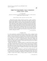
Fig. 1: Correlation functions 〈 W (l) 〉 , 〈 W (l)W (l) 〉 , and 〈 W (l)W (l)W (l) 〉 .
5

1) As Quantum Gravity
In this guise, we study a “field theory of universes.” We will introduce an operator (the
macroscopic loop operator) W (l, . . .) that creates universes of size l (1D and circular, in the
case of a 2D target space). The matrix model allows us to compute correlation functions
〈
W (l)
〉
,
〈
W (l) W (l)
〉
,
〈
W (l) W (l) W (l)
〉
, . . ., associated respectively with the Hartle–
Hawking wavefunction, with universe propagation, and with topology change (processes
depicted in fig. 1). The matrix model even allows both calculation of the effect of more
drastic topology changes and summation over topology–changing amplitudes.
2) As Critical String Theory
We will consider in detail the case for which (0.2) defines a flat Euclidean two dimensional
target spacetime with coordinates φ, X. Physical interpretations of the spacetime
theory require an analytic continuation to a spacetime of Minkowskian signature. There
are two choices for this continuation, but we shall argue that the clearest lessons for string
theory come from the c = 1 model that we will construct, with φ taken as the Liouville
coordinate, and t = −iX as the Minkowskian time coordinate.
t
Free
Strings
1
+log( )
µ
φ
Strongly
Coupled
Strings
Wall
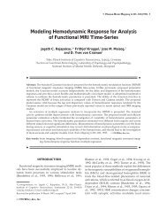
Fig. 2: Free, strong, and wall regions of the tachyon potential. At left, particles
are produced as tachyons scatter.
6

This exactly solvable spacetime background is a strange world. Since there are only
two spacetime dimensions, there are no transverse degrees of freedom. The only on-shell 1
field theoretic degree of freedom in the theory is that of a massless bosonic field T (t, φ),
called the “massless tachyon” (because the field T is mathematically analogous to a field
which is tachyonic for any string propagating in more than 2 spacetime dimensions, in
particular for the 26-dimensional bosonic string). Moreover, the world is spatially inhomogeneous.
We shall find (see eq. (5.14)) that the spacetime dilaton field has expectation
value 〈D〉 = Qφ/2, so that the string coupling varies with the spatial coordinate φ as
κ eff
= κ 0 e 1 2 Qφ . At φ = −∞, strings are free while at φ = +∞ strings are infinitely
strongly coupled. Finally, there is a cosmological constant term ∼ µe φ in the Liouville
path integral formulation of this theory that strongly suppresses contributions to path
integrals from large positive values of φ (we are assuming throughout these notes that the
cosmological constant satisfies µ > 0 , unless specified otherwise). Since the interaction
turns on exponentially there is effectively a wall located at φ = log 1/µ, often called “the
Liouville wall”, and the world looks as depicted in fig. 2. The most obvious physical experiment
we can perform in this world is to bounce our massless bosons off the wall. In
chapt. 13, we will show how to compute exactly the S-matrix for such scattering processes.
We are also able to compute the “flows” that relate physics in different (time-dependent)
backgrounds.
0.3. Review of reviews
Several reviews overlap different portions of the subject matter covered here. The
Liouville theory is reviewed in [7,8] and references therein. The matrix model technology
is reviewed in [9–14] (note that some sections here are adapted directly from [11]), the
c = 1 matrix model is reviewed in [15,16], and spacetime properties are emphasized in [17].
Other recent reviews are [18].
After treating the necessary preliminaries, our viewpoint here is largely complementary
to the other treatments, placing an emphasis on the properties of macroscopic loops,
the Wheeler–DeWitt equation, and the scattering theory in D = 2 target space dimensions.
In chapters 1–5, we give an overview of the continuum ideas and formalism we shall
use for treating loops and states in conformal field theory, for understanding the classical,
1 The graviton and dilaton in 2 spacetime target dimensions have no on-shell degrees of freedom,
i.e. are not physical propagating particles.
7

semiclassical, and quantum Liouville theories, and for implementing the path integral and
canonical treatments of 2D Euclidean quantum gravity. In chapters 6–9, we focus on the
discretized approach to 2d quantum gravity and 2d string theory, and explain various features
of the matrix model approach. In chapters 10–14, we employ the techniques provided
by the discretized approach to calculate many of the continuum quantities introduced earlier.
In chapter 15, we assess our prospects for the future. Appendix A contains some
useful definitions and facts about some of the special functions used in these lectures.
Due to lack of spacetime, we will not be reviewing many other important works on
the subject of 2D gravity. These notes are a preliminary version of a book [19], 2 that
will contain much interesting material omitted from these lecture notes. We welcome
constructive comments concerning typos, inconsistent conventions, inconsistent references,
sign errors and conceptual errors in these notes.
1. Loops and States in Conformal Field Theory
We begin here with a review of how a loop in the context of conformal field theory
can be replaced by a sum of local operators. For simplicity we will restrict attention to the
Gaussian model. The intuition from this example will be essential to our later extraction
of correlation functions from macroscopic loop amplitudes.
1.1. Lagrangian formalism
For simplicity, consider the standard c = 1 Gaussian model,
∫
S = ∂X ∂X , (1.1)
Σ
where Σ is a surface perhaps with handles and boundaries. The objects of interest are the
path integrals
∫
DX(z, ¯z) e −S O i (p i ) , (1.2)
where we integrate over maps X : Σ → IR.
The space of local operators is spanned by expressions of the form
∏
i
O ∼ P(∂X, ∂ 2 X, . . . ; ∂X, ∂ 2 X, . . .) e ikX(z,¯z) ,
(1.3)
2 the modest expenditure for which will be amply rewarded by the substantial further enlightenment
contained therein.
8

where P is a polynomial and the expression is suitably normal-ordered. When X is a
periodic variable, i.e. a map X : Σ → S 1 , then additional considerations apply: k is
quantized and there are winding modes which allow the definition of a more subtle theory
with an extra zero mode, leading to “magnetic” and “electric” quantum numbers. See [20]
for more details.
1.2. Hamiltonian formalism
In the radial Hamiltonian formalism (for a review, see e.g. [20]) we decompose the
fields into modes,
i∂X = ∑ α n z −n−1 ,
[α n , α m ] = n δ n+m
i∂X = ∑ ᾱ n ¯z −n−1 , [ᾱ n , ᾱ m ] = n δ n+m .
(1.4)
The stress-energy tensor T = − 1 2 (∂X)2 defines a Virasoro algebra and radial propagation
is generated by the Hamiltonian L 0 + ¯L 0 .
In terms of the Fock space
{∏
}
F p = Span (α −n ) m n
|p〉 n > 0, m n ≥ 0
n
(1.5)
α 0 |p〉 = p |p〉 α n |p〉 = 0 (n > 0) ,
we see that the states of the theory lie in a Hilbert Space of the form
H = ⊕ p,¯p N p,¯p F p ⊗ F¯p . (1.6)
Alternatively, we can think of the Hilbert space as the space of wavefunctionals Ψ[X(σ)].
(More precisely, we may introduce the loop space LIR and, with an appropriate measure,
the Hilbert space is simply the space H = L 2 (LIR) of square integrable maps of loops into
IR.)
Exercise. Coherent states
If we decompose
∑ ∑
X(σ) = x 0 + e inσ x n + e inσ ¯x n , (1.7)
n>0
n 0; α n ↔ ∂/∂x n ,
for n < 0; and similarly for ᾱ and ¯x, translate the Fock space states (1.5) into wavefunctionals
Ψ[X(σ)].
9

The Lagrangian and Hamiltonian formalisms are related by the so-called “operator
formalism”. The basic idea is that the neighborhood of any point on the surface Σ locally
looks like the complex plane and information about the rest of the surface may be
summarized in a state at infinity.
1.3. Equivalence of states and operators
One of the basic properties of conformal field theory is the one-to-one correspondence
between operators O and states |O〉.
To map operators → states, we associate the state |O〉 to the operator O(z, ¯z) according
to
O ↦→ |O〉 ≡ lim
z,¯z→0 O(z, ¯z)|0〉 . (1.8)
Equivalently, we can create a state by performing a path integral on a hemisphere D.
To evaluate such a path integral, the boundary conditions for the field X(z, ¯z) must be
specified on the equator, parametrized here by σ, and the value of the path integral defines
the wavefunction Ψ[X(σ)] (i.e. the wavefunction for the identity operator). Insertion of an
operator O on the hemisphere D gives the wavefunction Ψ O for the operator O,
[ ]
Ψ O X(σ) =
(1.9)
Using the equivalence between the Fock space and wavefunctional descriptions of the states,
the two descriptions (1.8) and (1.9) of the operator ↦→ state maps are easily seen to be
O
equivalent: namely 〈 X(σ) ∣ ∣ O
〉
= ΨO
[
X(σ)
]
(where
〈
X(σ)
∣ ∣ is a basis of eigenstates of the
operator X(σ) in the Fock space representation).
Exercise. Wavefunctions from path integrals
Consider a disk of radius r in the complex plane, centered at z = 0, and consider
the path integral (1.9) with boundary condition
∑ ∑
X(σ) = x 0 + e inσ x n + e inσ ¯x n (1.10)
n>0
n

where the constant C is determined by imposing some normalization condition.
b) Why can this be identified with the state |0〉 ?
c) Repeat this exercise to calculate the wavefunction for some other simple operators.
d) Describe the wavefunction associated to states created by local operators of the
form (1.3).
Expansion of loops in terms of local operators
Having described the operator ↦→ state mapping, now we wish to consider the inverse
state ↦→ operator mapping. To “insert a state” into the path integral, we cut a hole of
radius r out of the surface Σ, and insert a state with some wavefunction Ψ [ X(σ) ] on
the boundary of the hole (i.e. use Ψ [ X(σ) ] as the weight factor in the functional integral
over X(σ)).
We shall see that the new path integral is equivalent to that obtained by
inserting a local operator into (1.2), thus providing a states → operators mapping. The
mapping Ψ O ↦→ O is clearly linear and one-to-one, but to show that there is moreover an
isomorphism between states and operators, we need to show that every state is equivalently
represented by an operator insertion. The basic idea, physically, is to take a state inserted
on a hole and by conformal invariance shrink the hole to arbitrarily small size. Since an
infinitesimally small hole has the same effect as a local operator, the insertion of a state on
the boundary of a hole in the path integral is equivalent to the insertion of some operator.
In formulae, the states ↦→ operators mapping equates the insertion of a little hole of
radius r on any surface Σ in state |Ψ〉 with the insertion of a sum of operators at the center
of the hole,
W Ψ (r) ≡ ∑ i
〈O i |Ψ〉 r ∆ i+ ¯∆ i
O i . (1.12)
Here O i (z, ¯z) is a basis of local operators diagonalizing L 0 + L 0 , and W Ψ (r) is an operator
that inserts a macroscopic loop of size r with wavefunction Ψ [ X(σ) ] .
Example: Annular path integral.
Consider the path integral on a sphere with two holes, or, after a conformal transfor-
11

mation, on an annulus. This is given in the operator formalism by
r=1
Ψ 2
(1.13)
where ∣ ∣W Ψ1 (r) 〉 is the state associated to the local operator W Ψ1 (r). For more details on
the operator formalism, see e.g. [21–23].
Our goal is to calculate macroscopic loop amplitudes in 2D gravity. Current matrix
model technology will allow this only for some very specific states |Ψ〉, but these states will
have overlaps with sufficiently many interesting operators that much useful information can
be extracted. To provide a physical framework for interpreting the matrix model results,
we shall first investigate in the next two chapters the spectrum of Liouville theory and of
2D gravity.
r
= 〈Ψ
Ψ 1
= ∑
= ∑
= 〈
1.4. Gaussian Field with a Background Charge
For later comparison with the Liouville results, we give here a brief overview of gaussian
conformal field theory in the presence of a background charge, also known as Chodos–
Thorn/Feigin–Fuks (CTFF) theory. We consider the action
∫
S CTFF =
The additional term leads to the modified stress-energy
d 2 z √ ( 1 ĝ
8π ( ˆ∇φ) 2 + iα )
0
4π φR(ĝ) . (1.14)
T = − 1 2 ∂φ∂φ + iα 0 ∂ 2 φ , (1.15)
which generates a Virasoro algebra with central charge
c = 1 − 12α 2 0 .
We see that the effect of the extra term in (1.15) is to shift c < 1 for α 0 real. Since the
stress-energy tensor in (1.15) has an imaginary part, the theory it defines is not unitary
12

for arbitrary α 0 . For particular values of α 0 , it turns out to contain a consistent unitary
subspace.
Taking the operator product with the modified T of (1.15), we find that the conformal
weight of e βφ is shifted to ∆ = 1 2 β(β−2α 0). The same conformal weights would be inferred
from two-point functions calculated in the presence of a ‘background charge’ − √ 2α 0 at
infinity, so the modification of T (z) in (1.15) is interpreted as the presence of such a
background charge. This formalism was originally used by Chodos and Thorn in [24], and
was more recently revived by Feigen and Fuks in a form used in [25] to calculate correlation
functions of the c < 1 conformal field theories.
Exercise. Momentum Shift from Background Charge
Consider a Gaussian field with background charge Q = 2iα 0 . Derive the relation
ip φ = α − Q 2 , (1.16)
for the momentum p φ of the state created by the vertex operator exp(αφ) by considering
the state created by the path integral on the disk, analogous to the example of the
Gaussian model in (1.9).
2. 2D Euclidean Quantum Gravity I: Path Integral Approach
In this chapter, we shall consider the implementation of quantum gravity as a theory
which makes precise and well-defined sense out of a path integral over metrics on some
spacetime.
2.1. 2D Gravity and Liouville Theory
Using the principle of general covariance, any quantum field theory S matter [X i ] in any
number of dimensions may be coupled to gravity, resulting in an action S[g, X i ], where X i
refer to “matter” fields in the theory and g is the metric.
Classically, the theory S[g, X i ] with gravity coupling in two dimensions is always a
conformal field theory. To see this, recall that the stress energy tensor of the theory is
δ
δg αβ S = T αβ . Defining the Liouville mode as the overall scale of the metric, g = e γφ ĝ,
we see that the Liouville equation of motion is T α α = 0. This defines a classical conformal
field theory. In two dimensions, we may pass to local complex coordinates and write this
equation as T z¯z = 0. Conservation of energy-momentum then shows that the theory has a
holomorphic energy momentum tensor T zz = T (z).
13

Quantum mechanically, we try to understand the (Euclidean) quantum gravitational
path integrals
〈O 1 . . . O n 〉 = 1 Z
∫
∫
Dg DX
vol(Diff ) e−κ R−µA−S[X] O 1 . . . O n , (2.1)
where O i are generally covariant operators. By fixing a conformal gauge g ab
= e φ δ ab ,
Polyakov [2] observed that the matter/gravity theory could be written as a coupled tensor
product of Liouville theory and the “matter” theory S matter . The passage to conformal
gauge necessarily introduces the Faddeev–Popov reparametrization ghosts. At a formal
level, the gauge invariance of the theory, expressed as the independence of the integral
(2.1) to Weyl transformations of the gauge slice, implies that the coupling of Liouville and
matter theories is itself a conformal field theory. If the original matter theory was not
conformal, however, then the resulting theory will not be a simple tensor product.
Example 1: Coupling the massive Ising model
∫
S =
¯ψ∂ψ + m ¯ψψ (2.2)
to gravity results in the lagrangian
∫ ∫
√g ( )
S = ¯ψDψ + m ¯ψψ +
d 2 z √ ( 1 ĝ
8π ( ˆ∇φ) 2 + µ
8πγ 2 eγφ + Q )
8π φR(ĝ) , (2.3)
where D is the covariant derivative (i.e. includes the spin connection).
Example 2: Coupling the massive sine-Gordon model
to gravity results in the lagrangian
∫
S =
+
∫
d 2 z √ ( 1 ĝ
8π ( ˆ∇X) 2 + m cos(pX/ √ )
2)
d 2 z √ ( 1 ĝ
8π ( ˆ∇X) 2 + me ξφ cos(pX/ √ )
2)
∫
d 2 z √ ( 1 ĝ
8π ( ˆ∇φ) 2 + µ
8πγ 2 eγφ + Q )
8π φR(ĝ)
.
(2.4)
(2.5)
In both examples, we will see that Q and γ are fixed by general covariance. The
remarkable property of Liouville theory that allows it to associate an arbitrary quantum
field theory with some conformal field theory deserves to be better understood.
14

2.2. Path integral approach to 2D Euclidean Quantum Gravity
The first success of the discretized (matrix model) approach, the focus of our later
chapters here, was to reproduce the critical exponents predicted from continuum (Liouville)
methods. (In fact the coincidence of results served to give post-facto verification of both
methods.) In this section we review the latter continuum methods from a fairly formal
point of view. A more physical point of view will appear in the next chapter.
String susceptibility Γ str
We consider the continuum partition function
∫
Z =
Dg DX
vol(Diff ) e−S M(X; g) − µ 0
8π
∫
d 2 ξ √ g
, (2.6)
where S M is some conformally invariant action for matter fields coupled to a two dimensional
surface Σ with metric g, µ 0 is a bare cosmological constant, and we have symbolically
divided the measure by the “volume” of the diffeomorphism group (which acts as a local
∫
symmetry) of Σ . For the free bosonic string, we take S M = 1
8π d 2 ξ √ g g ab ∂ aX ⃗ · ∂bX
⃗
where the X(ξ) ⃗ specify the embedding of Σ into flat D-dimensional spacetime.
To define (2.6), we need to specify the measures for the integrations over X and g
(see, e.g. [26]). The measure DX is determined by requiring that ∫ D g δX e −‖δX‖2 g = 1,
where the norm in the gaussian functional integral is given by ‖δX‖ 2 g = ∫ d 2 ξ √ g δ ⃗ X · δ ⃗ X.
Similarly, the measure Dg is determined by normalizing ∫ D g δg e − 1 2 ‖δg‖2 g
= 1, where
‖δg‖ 2 g = ∫ d 2 ξ √ g (g ac g bd + 2g ab g cd ) δg ab
δg cd
, and δg represents a metric fluctuation at
some point g ij in the space of metrics on a genus h surface.
The measures DX and Dg are invariant under the group of diffeomorphisms of the
surface, but not necessarily under conformal transformations g ab
→ e σ g ab
. Indeed due to
the metric dependence in the norm ‖δX‖ 2 g , it turns out that
D
48π
D e σ gX = e
S L(σ)
Dg X , (2.7)
where
∫
S L (σ) =
d 2 ξ √ (
)
1
g
2 gab ∂ a σ∂ b σ + Rσ + µe σ
(2.8)
is known as the Liouville action. (This result may be derived diagrammatically, via the
Fujikawa method, or via an index theorem; for a review see [27].)
The metric measure Dg as well has an anomalous variation under conformal transformations.
To express it in a form analogous to (2.7), we first need to recall some basic facts
15

about the domain of integration. The space of metrics on a compact topological surface Σ
modulo diffeomorphisms and Weyl transformations is a finite dimensional compact space
M h , known as moduli space. (It is 0-dimensional for genus h = 0; 2-dimensional for h = 1;
and (6h − 6)-dimensional for h ≥ 2). If for each point τ ∈ M h , we choose a representative
metric ĝ ij , then the orbits generated by the diffeomorphism and Weyl groups acting on
ĝ ij generate the full space of metrics on Σ. Thus given the slice ĝ(τ), any metric can be
represented in the form
f ∗ g = e ϕ ĝ(τ) ,
where f ∗ represents the action of the diffeomorphism f : Σ → Σ.
Since the integrand of (2.6) is diffeomorphism invariant, the functional integral would
be infinite unless we formally divide out by the volume of orbit of the diffeomorphism
group. This is accomplished by gauge fixing to the slice ĝ(τ); the Jacobian that enters can
be represented in terms of Fadeev–Popov ghosts, as familiar from the analogous procedure
in gauge theory. We parametrize an infinitesimal change in the metric as
δg zz = ∇ z ξ z ,
δg¯z¯z = ∇¯z ξ¯z
(where for convenience we employ complex coordinates, and recall that the components
g = g¯zz z¯z
are parametrized by e ϕ ). The measure Dg at ĝ(τ) splits into an integration
[dτ] over moduli, an integration Dϕ over the conformal factor, and an integration
Dξ D ¯ξ over diffeomorphisms. The change of integration variables Dδg zz Dδg¯z¯z =
(det ∇ z det ∇¯z ) Dξ D ¯ξ introduces the Jacobian det ∇ z det ∇¯z for the change from δg to ξ.
The determinants in turn can be represented as
∫
det ∇ z det ∇¯z = Db Dc D¯b D¯c e − ∫ d 2 ξ √ g b zz ∇¯z c z − ∫ d 2 ξ √ g b¯z¯z ∇ z c¯z
∫
≡ D(gh) e −S gh(b, c, ¯b,
(2.9)
¯c) ,
where D(gh) ≡ Db Dc D¯b D¯c is an abbreviation for the measures associated to the ghosts
b, c, ¯b, ¯c; b zz is a holomorphic quadratic differential, and c z (c¯z ) is a holomorphic (antiholomorphic)
vector.
Finally, the ghost measure D(gh) is not invariant under the conformal transformation
g → e σ g, instead we have [2,26,27]
D eσ g(gh) = e − 26
48π S L(σ, g)
Dg (gh) , (2.10)
16

where S L is again the Liouville action (2.8). (In units in which the contribution of a single
scalar field to the conformal anomaly is c = 1, and hence c = 1/2 for a single Majorana–
Weyl fermion, the conformal anomaly due to a spin j reparametrization ghost is given by
c = (−1) F 2(1 + 6j(j − 1)). The contribution from a spin j = 2 reparametrization ghost is
thus c = −26.)
We have thus far succeeded to reexpress the partition function (2.6) as
∫
Z =
Choosing a metric slice g = e ϕ ĝ gives
[dτ] D g ϕ D g (gh) D g X e −S M − S gh − µ ∫
0
2π d 2 ξ √ g
.
D eϕĝϕ D eϕĝ(gh) D eϕĝX = J(ϕ, ĝ) Dĝϕ Dĝ(gh) DĝX ,
where the Jacobian J(ϕ, ĝ) is easily calculated for the matter and ghost sectors ( (2.7) and
(2.10) ) but not for the Liouville mode ϕ. The functional integral over ϕ is complicated by
the implicit metric dependence in the norm
∫
‖δϕ‖ 2 g = d 2 ξ √ ∫
g (δϕ) 2 =
d 2 ξ √ ĝ e ϕ (δϕ) 2 ,
since only if the e ϕ factor were absent above would the Dĝϕ measure reduce to that of a
free field.
In [28], it is simply assumed 3 that the overall Jacobian J(ϕ, ĝ) takes the form of an
exponential of a local Liouville-like action ∫ d 2 ξ √ ĝ (ã ĝ ab ∂ a ϕ∂ b ϕ + ˜b ˆRϕ + µe˜cϕ ), where ã,
˜b, and ˜c are constants that will be determined by requiring overall conformal invariance (˜c
is inserted in anticipation of rescaling of ϕ). With this assumption, the partition function
(2.6) takes the form
∫
Z = [dτ] Dĝϕ Dĝ(gh) DĝX e −S M(X, ĝ) − S gh (b, c, ¯b, ¯c; ĝ)
where the ϕ measure is now that of a free field.
· e − ∫ d 2 ξ √ ĝ (ã ĝ ab ∂ a ϕ∂ b ϕ + ˜b ˆRϕ + µe˜cϕ )
(2.11)
The path integral (2.11) was defined to be reparametrization invariant, and should
depend only on e ϕ ĝ = g (up to diffeomorphism), not on the specific slice ĝ.
Due to
3 Some attempts to justify this assumption may be found in [29]. In the next two chapters, we
shall see why this result should be expected from the canonical Hamiltonian point of view of [30].
17

diffeomorphism invariance, (2.11) should thus be invariant under the infinitesimal transformation
δĝ = ε(ξ)ĝ , δϕ = −ε(ξ) , (2.12)
and we can use the known conformal anomalies (2.7) and (2.10) for ϕ, X, and the ghosts to
determine the constants ã, ˜b, ˜c. Substituting the variations (2.12) in (2.11), we find terms
of the form
( D − 26 + 1
48π
˜b) ∫
+ d 2 ξ √ ∫
ĝ ˆR ε and (2ã − ˜b)
d 2 ξ √ ĝ ε ϕ ,
where the D − 26 on the left is the contribution from the matter and ghost measures DĝX
and Dĝ(gh), and the additional 1 comes from the Dĝϕ measure. Invariance under (2.12)
thus determines
˜b =
25 − D
48π
, ã = 1 2˜b . (2.13)
(In general we would substitute here D → c matter , where c matter is the contribution to the
central charge from the “matter” sector of the theory.)
Substituting the values of ã, ˜b into the Liouville action in (2.11) gives
∫
1
8π
d 2 ξ √ ( 25 − D ĝ ĝ ab ∂ a ϕ ∂ b ϕ + 25 − D
12
6
)
ˆR ϕ . (2.14)
∫ √
To obtain a conventionally normalized kinetic term 1
8π (∂ϕ) 2 12
, we rescale ϕ →
25−D ϕ.
(This normalization leads to the leading short distance expansion ϕ(z) ϕ(w) ∼ − log(z −
w).) In terms of the rescaled ϕ, we write the Liouville action as
where
∫
1
8π
d 2 ξ √ (
)
ĝ ĝ ab ∂ a ϕ ∂ b ϕ + Q ˆR ϕ , (2.15)
Q ≡
√
25 − D
3
. (2.16)
The energy-momentum tensor T = − 1 2 ∂ϕ∂ϕ+ Q 2 ∂2 ϕ derived from (2.15) has leading short
distance expansion T (z)T (w) ∼ 1 2 c Liouville /(z − w)4 + . . ., where c Liouville
= 1 + 3Q 2 . Note
that if we substitute (2.16) into c Liouville
and add an additional c = D −26 from the matter
and ghost sectors, we find that the total conformal anomaly vanishes,
c matter + c Liouv + c ghost = D + (26 − D) − 26 = 0
18

(consistent with the required overall conformal invariance).
It remains to determine the coefficient ˜c in (2.11). We have since rescaled ϕ, so we
write instead e γϕ and determine γ by the requirement that the physical metric be g = ĝ e γϕ .
Geometrically, this means that the area of the surface is represented by ∫ d 2 ξ √ ĝ e γϕ . γ
is thereby determined by the requirement that e γϕ behave as a (1,1) conformal field (so
that the combination d 2 ξ e γϕ is conformally invariant). For the energy-momentum tensor
mentioned after (2.16), the conformal weight 4 of e γϕ is
∆(e γϕ ) = ∆(e γϕ ) = − 1 2γ(γ − Q) . (2.17)
Requiring that ∆(e γϕ ) = ∆(e γϕ ) = 1 determines that
Q = 2/γ + γ . (2.18)
Using (2.16) and solving for γ then gives 5
γ = √ 1 (√ √ ) Q
25 − D − 1 − D = 12 2 − 1 √
Q
2
2 − 8 . (2.19)
For spacetime embedding dimension d ≤ 1, we find from (2.16) and (2.19) that Q and
γ are both real (with γ ≤ Q/2). The D ≤ 1 domain is thus where the Liouville theory is
well-defined and most easily interpreted. For D ≥ 25, on the other hand, both γ and Q are
imaginary. To define a real physical metric g = e γϕ ĝ, we need to Wick rotate ϕ → −iϕ.
(This changes the sign of the kinetic term for ϕ. Precisely at D = 25 we can interpret
X 0 = −iϕ as a free time coordinate. In other words, for a string naively embedded in 25
flat euclidean dimensions, the Liouville mode turns out to provide automatically a single
timelike dimension, dynamically realizing a string embedded in 26 dimensional Minkowski
spacetime. In general for D ≥ 25, we must have c Liouville
< 1 and the kinetic term of the
Liouville field changes sign. The conformal mode of the metric in Euclidean space is a
“wrong sign” scalar field analogous to the conformal mode in four-dimensional Euclidean
4 Recall that ∆ is given by the leading term in the operator product expansion T (z) e γϕ(w) ∼
∆ e γϕ /(z − w) 2 +. . . . Recall also that for a conventional energy-momentum tensor T = − 1 2 ∂ϕ∂ϕ,
the conformal weight of e ipϕ is ∆ = ∆ = p 2 /2.
5 One method for choosing the root for γ is to make contact with the classical limit of the
Liouville action. Note that the effective coupling in (2.14) goes as (25 − D) −1 so the classical limit
is given by D → −∞. In this limit the above choice of root has the classical γ → 0 behavior. We
shall discuss this issue further in the next chapter.
19

quantum gravity [31], so it would be useful to make sense of this case (if possible). Finally,
in the regime 1 < D < 25, γ is complex, and Q is imaginary. As we shall see later in lurid
detail, this problem is equivalent to the cosmological constant becoming a macroscopic
state operator. Sadly, it is not yet known how to make sense of the Liouville approach for
the regime of most physical interest.
A useful critical exponent that can be calculated in this formalism is the string susceptibility
Γ str . We write the partition function for fixed area A as
∫
Z(A) = Dϕ DX e −S ∫
δ(
d 2 ξ √ )
ĝ e γϕ − A , (2.20)
where for convenience we now group the ghost determinant and integration over moduli
into DX. We define a string susceptibility Γ str by
and determine Γ str by a simple scaling argument.
Z(A) ∼ A (Γ str−2)χ/2−1 , A → ∞ , (2.21)
(Note that for genus zero, we have
Z(A) ∼ A Γ str−3 .) Under the shift ϕ → ϕ + ρ/γ for ρ constant, the measure in (2.20) does
not change. The change in the action (2.15) comes from the term
∫
Q
d 2 ξ √ ĝ
8π
ˆR ϕ → Q ∫
d 2 ξ √ ĝ
8π
ˆR ϕ + Q ∫
ρ
d 2 ξ √ ĝ
8π γ
ˆR .
∫
Substituting in (2.20) and using the Gauss-Bonnet formula 1
4π d 2 ξ √ ĝ ˆR = χ together
with the identity δ(λx) = δ(x)/|λ| gives Z(A) = e −Qρχ/2γ−ρ Z(e −ρ A). We may now
choose e ρ = A, which results in
Z(A) = A −Qχ/2γ−1 Z(1) = A (Γ str−2)χ/2−1 Z(1) ,
and we confirm from (2.16) and (2.19) that
Γ str = 2 − Q γ = 1 12(
D − 1 −
√
(D − 25)(D − 1)
)
. (2.22)
In the nomenclature of [21], so-called “minimal conformal field theories” (those with a
finite number of primary fields) are specified by a pair of relatively prime integers (p, q) and
have central charge D = c p,q = 1 − 6(p − q) 2 /pq. The unitary discrete series, for example,
is the subset specified by (p, q) = (m + 1, m). After coupling to gravity, the general (p, q)
model has critical exponent Γ str = −2/(p + q − 1). Notice that Γ str = −1/m for the values
D = 1 − 6/m(m + 1) ) of central charge in the unitary discrete series. (In general, the m th
20

order multicritical point of the one-matrix model will turn out to describe the (2m − 1, 2)
model (in general non-unitary) coupled to gravity, so its critical exponent Γ str = −1/m
happens to coincide with that of the m th member of the unitary discrete series coupled
to gravity.) Notice also that (2.22) ceases to be sensible for D > 1, an indication of a
“barrier” at D = 1 that has already appeared and will reappear in various guises in what
follows. 6
Dressed operators / dimensions of fields
Now we wish to determine the effective dimension of fields after coupling to gravity.
Suppose that Φ 0 is some spinless primary field in a conformal field theory with conformal
weight ∆ 0 = ∆(Φ 0 ) = ∆(Φ 0 ) before coupling to gravity. The gravitational “dressing”
can be viewed as a form of wave function renormalization that allows Φ 0 to couple to
gravity. The dressed operator Φ = e αϕ Φ 0 is required to have dimension (1,1) so that it
can be integrated over the surface Σ without breaking conformal invariance. (This is the
same argument used prior to (2.19) to determine γ). Recalling the formula (2.17) for the
conformal weight of e αϕ , we find that α is determined by the condition
∆ 0 − 1 α(α − Q) = 1 . (2.23)
2
We may now associate a critical exponent ∆ to the behavior of the one-point function
of Φ at fixed area A,
F Φ (A) ≡ 1 ∫
Z(A)
Dϕ DX e −S δ( ∫
d 2 ξ √ ĝ e γϕ − A) ∫
d 2 ξ √ ĝ e αϕ Φ 0 ∼ A 1−∆ . (2.24)
This definition conforms to the standard convention that ∆ < 1 corresponds to a relevant
operator, ∆ = 1 to a marginal operator, and ∆ > 1 to an irrelevant operator (and in
particular that relevant operators tend to dominate in the infrared, i.e. large area, limit).
6 The “barrier” occurs when coupling gravity to D = 1 matter in the language of non-critical
string theory, or equivalently in the case of d = 2 target space dimensions in the language of
critical string theory. So-called non-critical strings (i.e. whose conformal anomaly is compensated
by a Liouville mode) in D dimensions can always be reinterpreted as critical strings in d =
D + 1 dimensions, where the Liouville mode provides the additional (interacting) dimension.
(The converse, however, is not true since it is not always possible to gauge-fix a critical string and
artificially disentangle the Liouville mode (see e.g. [32]).)
21

To determine ∆, we employ the same scaling argument that led to (2.22). We shift
ϕ → ϕ + ρ/γ with e ρ = A on the right hand side of (2.24), to find
F Φ (A) = A−Qχ/2γ−1+α/γ
A −Qχ/2γ−1 F Φ (1) = A α/γ F Φ (1) ,
where the additional factor of e ρα/γ = A α/γ comes from the e αφ gravitational dressing of
Φ 0 . The gravitational scaling dimension ∆ defined in (2.24) thus satisfies
∆ = 1 − α/γ . (2.25)
Solving (2.23) for α with the same branch used in (2.19),
α = 1 2 Q − √
1
4 Q2 − 2 + 2∆ 0 = 1 √
12
(√
25 − D −
√
1 − D + 24∆0
)
(2.26)
(for which α ≤ Q/2, and α → 0 as D → −∞). Finally we substitute the above result for
α and the value (2.19) for γ into (2.25), and find 7
∆ =
√ 1 − D + 24∆0 − √ 1 − D
√
25 − D −
√
1 − D
. (2.27)
We can apply these results to the (p, q) minimal models [21] mentioned after (2.22).
These have a set of operators labelled by two integers r, s (satisfying 1 ≤ r ≤ q − 1, 1 ≤
s ≤ p − 1) with bare conformal weights ∆ 0 = ( (pr − qs) 2 − (p − q) 2) /4pq (we take p > q).
Coupled to gravity, these operators have dressed Liouville exponents
1 − ∆ r,s = α r,s
γ
p + q − |pr − qs|
=
2q
1 ≤ r ≤ q − 1, 1 ≤ s ≤ p − 1 (2.28)
(p − q)2
(note also that c = 1 − 6
pq
=⇒ γ =
√
2q
p ,
√ √
2p 2q
Q = q + p
)
,
in agreement with the weights determined from the (p, q) formalism (to be discussed in
sections 7.4 and 7.7 ) for the generalized KdV hierarchy (see e.g. [34,35]).
7 We can also substitute α = γ(1 − ∆) from (2.25) into (2.23) and use − 1 γ(γ − Q) = 1 (from
2
before (2.19)) to rederive the result ∆−∆ 0 = ∆(1−∆)γ 2 /2 for the difference between the “dressed
weight” ∆ and the bare weight ∆ 0 [33].
22

3. Brief Review of the Liouville Theory
In this chapter, we touch briefly on some of the highlights of Liouville theory from
the viewpoint advocated in [7,17,8,36]. For other points of view on the Liouville theory,
see [37,38], and the sequence of works [39]. The classical Liouville theory was extensively
studied at the end of the nineteenth century in connection with the uniformization problem
for Riemann surfaces. We will sketch some of this in sections 3.2, 3.10 .
3.1. Classical Liouville Theory
We choose some reference metric ĝ on a surface Σ. The Liouville theory is the theory
of metrics g on Σ, and the Liouville field φ is defined by
The action is
∫
S Liouville =
g = e γφ ĝ . (3.1)
d 2 z √ ( 1 ĝ
8π ( ˆ∇φ) 2 + Q )
8π φR(ĝ) + µ ∫
8πγ 2
d 2 z √ ĝ e γφ , (3.2)
very similar to the background–charge theory (1.14) with a pure imaginary background
charge Q = 2iα 0 . The interaction given by µ (the “cosmological constant” term), while
soft, will be seen to have profound effects on the theory. For the particular choice
Q = 2/γ , (3.3)
the action (3.2) defines a classical conformal field theory, invariant under the Weyl transformations
ĝ → e 2ρ ĝ γφ → γφ − 2ρ . (3.4)
Remark: The linear shift in φ under a conformal transformation shows that φ can be
interpreted as a Goldstone boson for broken Weyl invariance (broken by the choice of ĝ).
Exercise. Classical Liouville theory
a) Using the transformation properties of the Ricci scalar in two dimensions,
R[e 2ρ ĝ] = e −2ρ( R[ĝ] − ˆ∇ 2 2ρ ) , (3.5)
compute the change in the action (3.2) under (3.4), and show that for Q = 2/γ the
change is independent of φ (so doesn’t affect the classical equations of motion).
b) Show that the classical equations of motion for (3.2) may be expressed as
i.e. they describe a surface with constant negative curvature.
R[g] = − 1 2 µ , (3.6)
(We take µ positive.)
Using again (3.5) (in the form R[g] = e −γφ( R[ĝ] − ˆ∇ 2 γφ ) , with φ as in (3.1)), note that
(3.6) is explicitly invariant under (3.4).
23

The stress-energy tensor following from (3.2), T µν
Feigin–Fuks form
T z¯z = 0
T zz = − 1 2 (∂φ)2 + 1 2 Q∂2 φ
= −2π δS
δg µν , takes the familiar
(3.7)
T¯z¯z = − 1 2 (∂φ)2 + 1 2 Q∂2 φ ,
where we have used the equations of motion in the first line.
Since φ is a component of a metric, its transformation law under conformal transformations
z → w = f(z),
φ → φ + 1 γ log ∣ ∣∣ dw
dz
∣ 2 , (3.8)
is more complicated than that of an ordinary scalar field. In particular, the U(1) current
∂ z φ measuring the Liouville momentum transforms as
and the stress tensor T zz transforms as
∂ z φ → dw
dz ∂ wφ + d 1
∣ ∣∣
dz γ log dw
∣ , (3.9)
dz
T zz →
( dw
) 2Tww
+ 1 S[w; z] . (3.10)
dz γ2 The object S[w; z] is called the “Schwartzian derivative” and has many equivalent definitions.
8 Combining (3.7) and (3.9), we see that
S[w; z] = − 1 (
∂ z log∣ dw
) 2 ∣
d2
∣ ∣∣ + 2 dz dz log dw
2 ∣
dz
= T zz
(φ = log∣ dw
)
∣
(3.11)
dz
= w′′′
w ′ − 3 ( w
′′ ) 2
.
2 w ′
The unusual transformation laws (3.9) and (3.10) have counterparts in the quantum theory,
where they result in shifted formulae for conformal charges and weights in Liouville theory.
8 It may be considered, for example, as the integrated version of the conformal anomaly, or it
may be defined in terms of “projective connections.” For a discussion of the latter concept see
[40].
24

3.2. Classical Uniformization
The central theorem in classical Liouville theory is the uniformization theorem that
characterizes Riemann surfaces.
Uniformization Theorem: Every Riemann surface Σ is conformally equivalent to
1) CP 1 , the Riemann sphere, or
2) H, the Poincaré upper half plane, or
3) A quotient of H by a discrete subgroup Γ ⊂ SL(2, IR) acting as Möbius transformations.
The first proofs of the uniformization theorem were based on the existence of solutions
to the classical field equations (3.6); the standard proofs use potential theory and are
nonconstructive (see [41]).
The upper half plane supports the standard solution of the Liouville equation, namely
the Poincaré metric:
ds 2 = e γφ |dz| 2 = 4 µ
1
(Im z) 2 |dz|2 , (3.12)
a constant negative curvature solution to (3.6). This metric is invariant under the Möbius
transformations
z → az + b , a, b, c, d ∈ IR, ad − bc = 1 (3.13)
cz + d
(i.e. the group P SL(2, IR) = SL(2, IR)/ Z 2 ), and thus descends to a metric
ds 2 = e γφ |dz| 2 = 4 µ
∂A ∂B
(
A(z) − B(¯z) ) 2 |dz|2 (3.14)
on the Riemann surface X = H/Γ for some locally defined (anti-)holomorphic functions
A(z) ( B(¯z) ) . In general, when we quotient H by the action of a discrete group Γ to define
a space X = H/Γ, there is a natural projection π : H → X and an “inverse” map
known as the “uniformizing map”.
Exercise. Classical energy-momentum
T zz = 0.
f : X → H , (3.15)
a) Evaluate the energy-momentum tensor for the Poincaré metric and show that
b) Let f : X → H be the uniformizing map as in (3.15). Show that the solution
(3.14) to the field equations has energy-momentum
with S[f; z] as in (3.11).
T zz = 1 S[f; z] , (3.16)
γ2 25

Note that the uniformizing map (3.15) is not well-defined. If we continue the values of
f from some coordinate patch around a nontrivial cycle, then f will change by the action
of T ∈ Γ. The nature of the surface near such a nontrivial curve depends on the nature of
the conjugacy class of T , in turn classified by the value of the trace. There are three types
of conjugacy classes in SL(2, IR):
1) elliptic: |Tr T | < 2 (T conjugate to ( cos λ sin λ
− sin λ cos λ)
) ,
2) parabolic: |Tr T | = 2 (T conjugate to ( 1 λ
0 1)
) , and
3) hyperbolic: |Tr T | > 2 (T conjugate to ( cosh λ sinh λ
sinh λ cosh λ)
) .
In cases 1,2), the nontrivial curve surrounds a puncture on the surface. In case 3), the
curve surrounds a handle. See [17] for further discussion.
Exercise.
a) Show that the Schwartzian derivative is invariant under independent Möbius
transformation of either z or f.
b) Show that although the uniformizing map is not globally defined, the energymomentum
(3.16) is nonetheless well-defined.
3.3. Quantum Liouville Theory
It is more subtle that the theory (3.2) is also a quantum conformal field theory.
If µ were zero and φ were a free field, we would immediately conclude that T defines
a Virasoro algebra with central charge c = 1 + 3Q 2 , that exponentials e αφ have conformal
weight − 1 2α(α−Q), and that these operators create states |α〉 on which we could construct
Feigin–Fuks modules. 9 Since φ is not a free field, 10 we must be more careful.
We proceed via canonical quantization, first passing from the complex z-plane to
cylindrical coordinates (t, σ) via z = e t+iσ , and expanding
φ(σ, t) = φ 0 (t) + ∑ i
(a n (t) e −inσ + b n (t) e inσ)
n
n≠0
Π(σ, t) = p 0 (t) + ∑ 1
)
(a n (t) e −inσ + b n (t) e inσ
4π
n≠0
.
(3.17)
9 A Feigin–Fuks module is a Fock space in which the Virasoro algebra is represented by an
energy-momentum tensor such as (3.7).
10 We will see that the operator product of two exponentials is not given by the free field
expression.
26

Here a † n = a −n , b † n = b −n , and we have the equal-time canonical commutation relations
[
an (t), b m (t) ] = n δ n,m . (3.18)
The energy-momentum tensor in canonical variables takes the form (again using the equations
of motion)
T +− = 0
T ±± = 1 8 (4πΠ ± φ′ ) 2 − Q 4 (4πΠ ± φ′ ) ′ + µ
8γ 2 eγφ + Q2
8 . (3.19)
The additive factor of Q 2 /8 in the above arises from the Schwartzian derivative in the
transformation properties (3.10) of T when mapping from the plane to the cylinder z →
(t, σ).
In [30], it was shown that the operators (3.19) satisfy a Virasoro algebra if
Q = 2 γ + γ (3.20)
(as we derived from another point of view in (2.18)). Calculating the [T, T ] commutator,
one finds indeed a central charge
c = 1 + 3Q 2 , (3.21)
and calculating commutators with T shows that exponentials e αφ have conformal weight
∆(e αφ ) = − 1 2 (α − Q/2)2 + Q 2 /8 . (3.22)
Note that if we impose the condition ∆(e αφ ) + ∆ 0 = 1, to dress an operator with bare
weight ∆ 0 , we rederive the KPZ equation (2.26).
It is useful to have an intuitive understanding of eqns. (3.20–3.22).
Note that by
rescaling φ → 1 γ
φ in (3.2), we identify γ with the coupling constant of the theory. The
semiclassical theory is thus defined by asymptotic expansion as γ → 0. We see that
(3.20) is the quantum version of the classical condition (3.3) for conformal invariance.
Similarly, (3.21) consists of a classical part (∝ Q 2 ∝ 1/γ 2 ) already visible in the classical
transformation law (3.10), plus a quantum conformal anomaly (c = 1), familiar for a
single scalar field. Finally, to understand (3.22) we note that the analog of (3.9) in the full
quantum theory is
∂ z φ → dw
dz ∂ wφ + d Q
∣ ∣∣
dz 2 log dw
∣ . (3.23)
dz
27

In particular, passing from the plane to the cylinder via the conformal transformation
w = log z we have ∂ z φ → (∂ w φ − Q/2)/z, so the momentum “shifts” by Q/2. The vertex
operators e αφ , inserted on the z-plane, create states with Liouville momentum p φ
given by
ip φ = α − Q 2 . (3.24)
(Note that “states” refer to quantization on the cylinder, and “Liouville momentum” refers
to the zero mode p 0 of Π in (3.17).) We see that the first term in (3.22) is simply 1 2 p2 φ ,
and the second term is the shift in the energy (relative to the Gaussian case) due to the
“extra” central charge.
The above formulae are valid for cosmological constant µ ≥ 0. It may seem curious
that the quantum formulae for µ > 0 are identical to those obtained for a free field, i.e.
with cosmological constant µ = 0 in (3.2). (N.B.: a translation of φ cannot transform
one case into the other.) Heuristically, we can understand this by noting that in the
worldsheet ultraviolet, φ → −∞, the interaction term disappears: Quantities such as c
and ∆, determined by the singular terms in operator product expansion, depend only on
the ultraviolet behavior of the theory.
3.4. Spectrum of Liouville Theory
We now proceed to study the Hilbert space of the theory, all of whose subtleties lie
in the zero modes φ 0 (t), p 0 (t). We can understand the physics of these degrees of freedom
by studying the action (3.2) for field configurations independent of σ, i.e., we study the
Liouville quantum mechanics
∫
S =
dt ( ˙φ 2 + µ γ 2 eγφ ) . (3.25)
The Hamiltonian H 0 = 1 2
∮
(T++ + T −− ), after substituting (3.19), takes the form
H 0 = − 1 2
( ∂
∂φ 0
) 2
+
µ
8γ 2 eγφ 0 +
1
8 Q2 . (3.26)
28

|ψ|
V
ϕ
Fig. 3: Particle wavefunctions in the exponential potential.
The spectrum of H 0 is easily understood. In the worldsheet ultraviolet, φ 0 ∼ −∞ (i.e.
at short physical distances), the potential disappears so that normalizable states behave
like plane waves, ψ E
∼ sin Eφ 0 , with energy 1 2 E2 + 1 8 Q2 . The exponential growth of the
potential prevents the “particle” at φ 0 from penetrating too far to the right, and hence
gives total reflections of any incoming wave. Because of the total reflection property there
is no distinction between states with +E and −E and we can therefore take E > 0. The
wavefunctions look as in fig. 3.
The circumference of the 1D “universe” in physical units is measured by the quantity
1
2
l = e
γφ 0
. (3.27)
Using l, it is moreover possible to give an exact description of the eigenstates of H 0 in
(
terms of Bessel functions. Changing variables to l, the eigenvalue equation H 0 ψ E
=
1
2 E2 + 1 8
)ψ Q2 E
becomes
(−(l ∂ ) (
∂l )2 + 4ˆµl 2 + Q2
Q
2 )
ψ
γ 2 E (l) =
γ + Ê2
ψ 2 2 E , (3.28)
where ˆµ = µ/(4γ 4 ) and Ê = √ 8E/γ.
We recognize (3.28) as the Bessel differential
equation. Imposing the boundary condition that ψ decays for large universes, l → ∞,
gives the eigenfunction
ψ E = 1 π
√Ê sinh πÊ KiÊ (2√ˆµl) , (3.29)
where K is the modified Bessel function. We have chosen a δ-function normalization for
the states,
∫ ∞
0
dl
l ψ E(l) ψ E
′ (l) = δ(E − E ′ ) . (3.30)
29

Exercise. The wall analogy
Show that the solutions ψ E behave asymptotically for φ 0 → −∞ as sin ( 1
γEφ 2 0 +
α(E) ) , where
α(E) = arg Γ(1 + iE) = 1 Γ(1 + iE)
log
2 Γ(1 − iE) .
For intuitive purposes, it is useful to replace the exponentially growing Liouville potential
by an infinite hard wall. Where should this wall be located for energies of order
E?
Now we proceed from the zero mode structure of the theory to construct the full
field theory. Combining the above discussion on zero modes with canonical quantization,
one expects [30] the Hilbert space (as a Vir ⊕ Vir representation space) of the Liouville
conformal field theory to take the form
∫ ∞
H = ⊕
0
dE F ∆(E) ⊗ F ∆(E) . (3.31)
Here F is a Feigin–Fuks module with weight ∆(E) = 1 2 E2 + 1 8 Q2 and central charge
c = 1 + 3Q 2 . Our notation on the r.h.s. of (3.31) is meant to indicate a direct integral of
Hilbert spaces [42]. Each Feigin–Fuks module is generated by adding oscillator excitations
to some primary state. As usual, this structure may be understood heuristically since in
the worldsheet ultraviolet (φ → −∞) the theory becomes free.
In a conventional conformal field theory we are able to associate each state in the
Hilbert space to an operator, and then determine the operator algebra of the theory. How
do we construct the vertex operators that create states in the space (3.31)? According to
(3.24), we might expect the primary fields of Liouville momentum p φ
= E to have quantum
vertex operators
V E (z, ¯z) = e αφ = e iEφ e 1 2 Qφ . (3.32)
At this point, however, we begin to encounter some of the confusing subtleties of Liouville
theory cum quantum gravity, as first emphasized in [7,8]: the operators (3.32) by no means
encompass all of the quantities of interest in the theory. For example, a natural quantity
in quantum gravity is the “volume of the universe,”
∫
A = e γφ√ ĝ , (3.33)
Σ
given by integrating the area operator e γφ . But comparing with (3.32), we see that this
operator has imaginary momentum and cannot correspond to a normalizable state (in
the sense of (3.30)). To obtain some insight into this puzzling observation, we return to
examine the semiclassical theory.
30

3.5. Semiclassical States
The semiclassical approximation is an important source of intuition for understanding
Liouville theory. Classical Liouville theory describes the geometry of negatively curved
surfaces (eq. (3.6)). Earlier, we identified γ with the coupling constant of the theory (by
rescaling φ → φ/γ), so the semiclassical limit is defined by γ → 0 asymptotics. In this
limit, we expect the above quantum states to correspond to specific constant curvature
surfaces, and this has been verified in detail [7,17]. Briefly, the σ-independent metric
e γφ(t) (dt 2 + dσ 2 ) = 4 µ
ε 2
sin 2 (εt) (dt2 + dσ 2 )
nπ
ε
< t <
(n + 1)π
ε
(3.34a)
(where z = e t+iσ and ε is a real number), is a solution to the Liouville equation (3.6) that
looks something like
hyperbolic:
(3.34b)
Exercise. Classical field energy
Use the energy momentum tensor (3.7) to show that the Liouville field configuration
(3.34) has classical energy 1 2 (ε2 /γ 2 ) + 1 8 Q2 .
Recalling that the quantum state ψ E of (3.28) has energy 1 2 E2 + 1 8 Q2 , this classical
field energy allows us to identify (3.34) as the semiclassical picture of the quantum state
ψ E for E = ε/γ.
As noted in sec. 3.2, there are three kinds of local behavior of a solution to the
classical Liouville equation, classified by the monodromy properties of A, B in (3.14). In
the solution (3.34a) above, we have A = z iε = B, thus giving an example of a hyperbolic
class. From the semiclassical point of view, we are naturally led to ask what quantum
states correspond to the other two classes, namely the elliptic and parabolic solutions.
These are given respectively by
ν 2
e γφ (dt 2 + dσ 2 ) = 4 µ sinh 2 (νt) (dt2 + dσ 2 ) t < 0
e γφ (dt 2 + dσ 2 ) = 4 1
µ t 2 (dt2 + dσ 2 ) t < 0 .
(3.35a)
31

Here ν is a real number. An important feature of the solutions (3.35a) is their equivalence
for both ±ν. These solutions look something like
elliptic, parabolic:
(3.35b)
and have energy − 1 2 (ν2 /γ 2 ) + 1 8 Q2 . Quantum mechanically, according to (3.28, 3.29) they
therefore correspond to states with imaginary momentum E = iν/γ. The corresponding
wavefunctions are of type K ν (l), ν real. These wavefunctions blow up (as l −|ν| ) at short
distances l → 0 and consequently might appear unphysical. On the contrary, as we saw at
the end of the previous section, operators corresponding to imaginary momentum states,
including for example the volume of the universe, appear quite naturally in 2D quantum
gravity and play an important role.
The distinction between normalizable and non-normalizable states in Liouville theory,
and the necessity to include the non-normalizable states in the theory, was first emphasized
by Seiberg in [7]. Motivated by the geometries illustrated above, the normalizable states
were labelled “macroscopic states,” and the non-normalizable states were labelled “microscopic
states”. Semiclassically, the macroscopic states do not have a well-defined insertion
point in the intrinsic geometry of the surface. The microscopic states, on the other hand,
correspond semiclassically to the elliptic geometry pictured in (3.35b), and thus to local
operators — the operator insertion in this case is localized at the tip of the “funnel.” We
discuss these issues further in sec. 4.3 below.
Exercise. Curvature Sources
z-plane:
a) Use the exponential map z = e t+iσ to transform the solutions (3.35) to the
e γφ dz d¯z = 16
µ
ν 2 (z¯z) ν dz d¯z
(1 − (z¯z) ν ) 2 z¯z
b) Show that the field φ solves the Liouville equation with source,
. (3.36)
1
4π ∆φ − µ
8πγ eγφ + 1 − ν
γ δ(2) (z) = 0 , (3.37)
i.e., such solutions have a source of curvature at z = 0.
32

c) Show that the solution corresponds to the choice of functions (in (3.14)):
A(z) = i zν + 1
z ν − 1
B(¯z) = −i ¯z ν + 1
¯z ν − 1 . (3.38)
d) Show that the monodromy when z circles around the puncture is the real elliptic
Möbius transformation
cos πνA(z) − sin πν
A(z) →
sin πνA(z) + cos πν . (3.39)
e) Show that a straight line through z = 0 is conformally mapped into an angle
πν, and hence we must have ν ≥ 0 on geometric grounds.
f) Repeat the above for the hyperbolic and parabolic cases.
3.6. Seiberg bound
Classically, the metrics (3.34, 3.35) are invariant under ν → −ν, E → −E. Quantum
mechanically, the wavefunctions K ν , K iE share this invariance, due to the total reflection
property of the Liouville “wall.” Turning on the wall by setting µ > 0 effectively halves
the states that exist in the (µ = 0) free spectrum.
In the DDK/KPZ formalism described in chapt. 2, on the other hand, the choice of
root in the KPZ formula (2.27) affects the scaling properties of the operator e αφ Φ 0 . Since
the Liouville interaction truncates the spectrum by half, we must choose a root. In [7,8],
it is argued that only those operators with
α ≤ 1 2 Q (3.40)
can exist. This choice of root has many distinguishing properties, some of which will be
noted in later sections:
1) This root gives a smooth semiclassical limit in quantum gravity, as we saw in sec. 2.2.
2) The area element is integrable only for sources satisfying (3.40). A related fact in terms
of deficit angles has appeared in part (e) in the exercise above (following (3.39)).
3) As we will see in the penultimate paragraph of sec. 4.3 , the Wheeler–DeWitt wavefunction
for a local operator in quantum gravity, related to the vertex operator V (φ)
by ψ(φ) = e − 1 2 Qφ V (φ), must be concentrated on l → 0, that is, where φ → −∞.
4) A closely related question is the nature of gravitational dressing (see sec. 2.2). Only
with the choice of root (3.40) do gravitationally dressed relevant/irrelevant operators
grow/decay in the worldsheet infrared.
33

5) As will be seen in sec. 5.4 below, the bound (3.40) has the following spacetime interpretation:
When scattering in a left half-space, incomers must be rightmovers and
outgoers must be leftmovers.
In addition, there is circumstantial evidence that (3.40) is correct:
1) In the matrix model, we will see that only scaling operators with scaling corresponding
to α ≤ Q/2 appear.
2) In the semiclassical calculations of [30], there are difficulties constructing correlation
functions of “wrong branch” operators.
3) In the SL(2, IR) quantum group approach pursued by Gervais and others, inverse
powers of the metric e −jγφ , 2j ∈ Z + , are easily constructed, while the positive powers
have thus far eluded construction.
The above reasoning is qualitative. While the Seiberg bound (3.40) is undoubtedly correct,
a precise mathematical understanding of the statement would be useful.
A common confusion
There are two distinct novelties in the description of the Hilbert space of Liouville
theory: (1) Vertex operators with α > 1 2Q do not exist. (2) States with real momentum
p φ
= E, which formally correspond to vertex operators with α = 1 2Q + iE, do not have a
correspondence with local operators. These two distinct points are often confused in the
literature. There is no (obvious) connection between the Seiberg bound, which specifies
the operators that exist, and the difficulty of localizing operators that correspond to states
|E〉 of energy 1 2 E2 + 1 8 Q2 .
An unresolved confusion
There is some confusion in the literature as to whether the states |E〉 have a correspondence
with vertex operators V E = e iEφ e 1 2 Qφ . Although the semiclassical pictures of
states (e.g. (3.34b)) makes any correspondence with local operators seem unlikely [7], we
shall find these operators necessary to formulate our scattering theory in two Minkowskian
dimensions. This problem is closely linked to the problem of time in string theory.
Exercise. Seiberg bound and semiclassical limits
Consider the minimal conformal field theories labelled by (2, 2m − 1) in the BPZ
classification, as mentioned after (2.22). Show that γ = 2/ √ 2m − 1 so that as m → ∞
the semiclassical approximation becomes valid. Note that the root chosen in sec. 2.2 on
the basis of the semiclassical limit coincides with that dictated by the bound (3.40).
34

3.7. Semiclassical Amplitudes
In the semiclassical approximation, we evaluate the amplitudes
〈∏ 〉 ∫
e α iφ(z i )
≡ [dφ] e ∏ −S Liouville[φ]
e α iφ
i
i
via the saddle point approximation by first solving the classical equation
1
4π ∆φ − µ
8πγ eγφ + ∑ i
(3.41)
α i δ (2) (z − z i ) = 0 . (3.42)
Integrating (3.42) over the surface Σ we find, since µ > 0, that a necessary condition for
the existence of a solution is
Exercise.
1
( 1
γ γ (2 − 2h) − ∑ )
α i < 0 . (3.43)
Derive (3.43) using the Gauss-Bonnet theorem, ∫ 1
4π R√ g = χ = 2 − 2h.
The particular combination
s ≡ Q 2γ χ − ∑ α i
γ , (3.44)
known as the KPZ exponent [33], plays an important role in the theory. Equation (3.43)
says that the semiclassical KPZ exponent (Q → 2/γ) is negative.
When s < 0, there is indeed a solution to (3.42), and we can expand around it to
evaluate (3.41). Near z = z i , it follows from (3.42) that
φ cl ∼ −α i log |z − z i | 2 (3.45)
for α i < 1/γ. For α = 1/γ we have instead
φ cl ∼ − 1 (
log |z − z i | 2 1
)
+ 2 log log . (3.46)
γ
|z − z i |
In either case, to write the semiclassical amplitudes we must excise disks B(r, z i ) around
z i of radius r (in the ĝ metric), and define the regularized action 11
S[φ cl ] ≡ lim
L −
r→0
(∫Σ−∪ ∑ i B(r,z i ) i
)
(∆ i + ∆ i ) log r
(3.47)
[7].
11 The need for these subtractions reflects the need for renormalization of the vertex operators
35

where ∆ i is the conformal weight of e α iφ . In terms of S, the leading γ → 0 asymptotics of
the correlator are given by
〈∏
e
α i φ(z i )〉
s.c.
∼ e −S[φ cl ] . (3.48)
There are also cases of interest with s ≥ 0, notably, for genus zero correlators of vertex
operators with small total “Liouville charge” ∑ α i . In these cases, as described in [7], we
can still perform semiclassical calculations by fixing the total area of the surface: we insert
δ( ∫ e γφ − A) into the path integral to ensure that (3.42) has a solution. We obtain the
A dependence of fixed area correlators by a scaling argument (similar to that used before
(2.22) and (2.25)): shifting φ → φ + 1 γ
log A gives
〈∏ 〉 〈∏ 〉
e α iφ(z i )
= A −1−s e
α i φ(z i )
i
A
A=1
, (3.49)
with s as in (3.44). To Laplace transform to fixed cosmological constant, we integrate
∫ ∞
0
dA
A A−s e −µA = µ s Γ(−s) . (3.50)
The UV divergence as A → 0 for s ≥ 0 (reflecting the absence of a classical solution
without the area constraint) plays an important role in speculations on the relation of free
field theory to the Liouville theory described in sections 3.9, 14.2, 14.3 below.
Using (3.49), the problem of calculating correlators is reduced to the case A = 1. The
semiclassical formulae for genus zero correlators are obtained by averaging over the space
of classical solutions. These solutions are obtained for s ≥ 0 by applying complex Möbius
transformations from the standard round-sphere metric
ds 2 = e γ ¯φ |dz| 2 = 16 µ
|dz| 2
(
1 + |z|
2 ) 2
(3.51)
(which, unlike (3.6), has positive curvature R = + 1 2
µ). The result is
〈∏ 〉 ∫
s.c.
e
α i φ(z i )
= d 2 a d 2 b d 2 c d 2 d δ (2) (ad − bc − 1) ∏ e α i ¯φ(z i )
A=1
i
= ∏ ( 16
) ∫ αi /γ ∞ ∫
dλ λ
µ
i
0 C d2 w ∏ (3.52)
1
(
i |λzi + w| 2 + λ −2) , 2α i /γ
where in the second line we have parametrized SL(2,C) elements by a unitary matrix times
an upper triangular matrix, and we have dropped the volume of SU(2). See [7] for more
details.
36

Semiclassical Seiberg Bound [7,8]
The semiclassical approach provides a key insight into the Seiberg bound (3.40). Consider
the classical equation (3.42) in the neighborhood of a vertex operator insertion. If
we neglect the cosmological constant term, the solution must behave as in (3.45). To check
if this is self-consistent, we insert (3.45) back into (3.42) and note that the neglected term
behaves as
e γφ ∼
1
|z − z i | 2α iγ . (3.53)
If α i γ > 1, the cosmological constant operator is not integrable at z = 0 and we expect
trouble.
Indeed, the careful considerations leading to the classification of solutions in
sec. 3.2 (following eq. (3.16)) show that there is no solution for α i > 1/γ ∼ Q/2. The
essential point is that too much curvature cannot be localized at a single point.
Here are two examples of semiclassical correlators:
Example 1: Consider the three-point function on the sphere,
〈
e
θ 1 φ/γ (z 1 , ¯z 1 ) e θ 2φ/γ (z 2 , ¯z 2 ) e θ 3φ/γ (z 3 , ¯z 3 ) 〉 , (3.54)
where θ i < 1 are considered to be O(1) as γ → 0 and ∑ i θ i > 2, so s < 0. The classical
solution is known in this case and is Möbius invariant. It follows immediately from (3.47)
and the transformation properties of circles under Möbius transformations that
〈
e
θ 1 φ/γ (z 1 , ¯z 1 ) e θ2φ/γ (z 2 , ¯z 2 ) e θ3φ/γ (z 3 , ¯z 3 ) 〉 C[θ i ]
∼ ∣
∣z ∆ 123
12
z ∆ 132
13
z ∆ 231
23
∣ 2 , (3.55)
where ∆ 123 = ∆ 1 + ∆ 2 − ∆ 3 , etc. The coefficient function C is generically nonzero. Sadly,
this example cannot be extended to higher point functions because the classical solutions
to Liouville theory are not known in explicit form, except in special cases which have the
punctures symmetrically located [43].
Example 2: Consider now the three-point function on the sphere, but with s ≥ 0 so we
must fix the area. Using the Möbius invariance of (3.52) gives
C[α i ] =
〈
e
α 1 φ (z 1 , ¯z 1 ) e α2φ (z 2 , ¯z 2 ) e α3φ (z 3 , ¯z 3 ) 〉 s.c.
∼ C[α i ]
A=1
|z ∆ 123
∫ ∞
∫
dλ
0 λ λ4(α 1+α 2 −α 3 )/γ
1
C d2 w (
|w| 2 + 1 ) 2α 1 /γ
= π 4
Γ(j 1 − j 2 − j 3 ) Γ(j 2 − j 3 − j 1 ) Γ(j 3 − j 1 − j 2 )
Γ(−2j 1 ) Γ(−2j 2 ) Γ(−2j 3 )
12
z ∆ 132
13
z ∆ 231
23
| 2
1
(
|w + λ 2 | 2 + 1 ) 2α 2 /γ
Γ(−j 1 − j 2 − j 3 − 1) ,
(3.56)
37

where j k ≡ −α k /γ. Strictly speaking, the integrals above converge only for ranges of j k
for which the arguments of all the Γ–functions in (3.56) are positive. As in ordinary string
theory, we define the amplitude at other values of j by analytic continuation.
Remarks:
1) The formula (3.52) has an interesting group-theoretical meaning. Defining j ≡ −α/γ,
the field e αφ transforms under SL(2,C) in the (j, j) representation of SL(2,C), hence
the suggestive notation. Group theoretically, the integral (3.55) computes the overlap
between a product of vectors in infinite-dimensional highest weight representations
and the trivial representation.
2) Analytically continuing j 3 to pure imaginary values, and taking the limit j 3 → 0, gives
the two-point function
〈e −j 1φ (z 1 , ¯z 1 ) e −j 2φ (z 2 , ¯z 2 )〉 = − iπ2
4
1
2j 1 + 1 δ(j 1 − j 2 )
1
|z 12 | 4∆ 1 , (3.57)
obtained in [7] by analytic continuation of the integration over the dilation subgroup
IR ∗ + ⊂ SL(2,C). For a further discussion of the subtleties of one- and two-point
functions, and their relations to the regularized volumes of IR ∗ + and SL(2,C), see
[7]. 12
3) Note that fields with j ∈ 1 2 Z + generically decouple. If all three fields satisfy j ∈ 1 2 Z + ,
then we recover the SU(2) fusion rules.
4) The two above examples make it clear that the Liouville correlators are entirely different
from the correlators of a Coulomb gas with a charge at infinity. In particular,
there is no Liouville charge conservation.
5) It is very unusual to have short distance singularities in the correlators of the classical
theory as we do in (3.56) and (3.57). This is due to the average over the noncompact
group SL(2,C), so we see again that the geometrical origin of the Liouville field
distinguishes it from an ordinary scalar field. Note that for the n ≥ 4 -point functions,
the operator products are typically smooth in the semiclassical correlator.
12 That Liouville two-point functions are diagonal in Liouville charges might have important
implications for the implementation of string field theory identities [44].
38

3.8. Operator Products in Liouville Theory
The existence of the Seiberg bound (3.40) dictates that the operator product expansion
in Liouville theory will be rather different from that in free field theory. Indeed it is not
clear that the notion of the operator product expansion is the correct language to use when
discussing Liouville correlators. Already in the semiclassical theory, we shall see that the
putative short distance behavior of correlators depends on global properties of the surface
and the “operator product expansion” appears to be nonlocal [7,8].
Fig. 4: Left: Insertion of operators e αφ and e βφ in a surface with boundary. Right:
the same operation on a higher genus surface.
Consider the state arising from the insertion of two vertex operators e αφ and e βφ on
a surface with boundary C as in the l.h.s. diagram of fig. 4, or, more generally, on a higher
genus surface as in the r.h.s. diagram of fig. 4. In the semiclassical approximation, the
state created by the surface on the boundary C has a wavefunction that depends on the
zero-mode φ 0 of φ as
ψ(φ 0 ) ∼ e αφ 0 +βφ 0 − 1 2 Qχφ 0 , (3.58)
where χ = 1 − 2h is the Euler character for the surface (with a single boundary).
α + β < 1 2 Qχ, then the wavefunction (3.58) is a real exponential diverging at φ 0 → −∞
(short distance). Then we may expect to replace the holes in the diagrams in fig. 4 each
by a sum of local (“microscopic”) operators, as in ordinary conformal field theory. Note
that since the three-point functions are generically nonzero, we would naively expect a
disastrous sum over operators with conformal dimensions unbounded from below.
If α + β > 1 2Qχ, on the other hand, then the state is normalizable and we certainly
cannot expand it in an operator product expansion of local operators. Instead the state
must be expanded in the normalizable macroscopic state operators. Thus, by sewing, the
surface amplitude must have the form
〈
e αφ(z,¯z) e βφ(z,¯z) · · ·〉 ∼
∫ ∞
0
dE c αβE |z − w| 2(E2 /2+Q 2 /8−∆ α −∆ β ) 〈E|Σ〉 , (3.59)
39
If

where |Σ〉 is a state created by the rest of the surface (as is standard in discussions of
the “operator formalism” [21–23]). If we interpret the integral in (3.59) as an OPE over
macroscopic vertex operators V E , then since we sum over operators with weights ∆ ≥
Q 2 /8, we see that the OPE is much softer than in ordinary CFT. This discussion can be
generalized.
The essential message is that while we may insert microscopic operators on a surface we
should only do so “externally.” We must factorize on macroscopic states. The factorization
on macroscopic states also ameliorates the disastrous sum noted above for α + β < 1 2 Qχ.
The essentially non-free field nature of the operator product expansion in Liouville
theory accounts for some unusual properties of the theory.
As one example, note that
since the Liouville theory is conformal for all µ > 0, the cosmological constant e γφ is
an exactly marginal operator.
This appears to conflict with the fact that its n-point
correlation functions are nonvanishing, since the standard obstruction to exact marginality
is the existence of a “potential” for such couplings. However, the standard discussion of
the obstruction to exact marginality does not apply because of the strange nature of the
operator product expansion. In later sections on string theory (sec. 5.6 ) we will see that
the unusual OPE of Liouville also has important consequences for the finiteness of the
theory and for the existence of an infinite dimensional space of background deformations.
3.9. Liouville Correlators from Analytic Continuation
In the past two years there has been very interesting progress in understanding Liouville
correlation functions via “analytic continuation in the number of operators.” The first
step in the calculation of continuum correlators was provided in [45], where the free field
formulation by zero mode integration of the Liouville field was established. The essential
idea is to treat the Liouville path integral measure as a free field measure and separate out
a zero-mode φ 0 via φ = φ 0 + ˆφ, so that [dφ] = [d ˆφ] dφ 0 . The integral over the zero mode is
∫ ∞
−∞
s ≡ 1 γ
∑
dφ 0 e
αi φ 0 e
−Qχφ 0
/2−Be γφ 0
(
1
2 Qχ − ∑ α i
)
= 1 Γ(−s) Bs
γ
B ≡ µ ∫ √ĝ
e
γ ˆφ .
8πφ 2
(3.60)
In references [46–49], it is proposed that when s ∈ Z + (so there is no negative curvature
solution) the ˆφ integral can be done using free field techniques. One then obtains a class
40

of amplitudes as “functions of s,” manipulates the s-dependence to reside solely in the arguments
of Γ-functions (through factorials) and then “analytically continues” to all values
of s using Γ(x + 1) as an analytic continuation of x! .
This curious procedure has scored many impressive successes. In particular [46], the
incorporation of the Liouville mode was shown to cancel the ghastly assemblage of Γ-
functions familiar from the conformal field theory result and reproduce the relatively simple
matrix model result for many continuum correlation functions. Additional genus zero
correlation functions for D ≤ 1 were computed in [48]. The genus one partition function
for the AD series was calculated via KdV methods in [50], and was confirmed from the
continuum Liouville approach in [51].
Attempts to justify the technique on physical grounds are based on arguments that
for s ∈ Z + , the coefficient of log µ in the correlation function is dominated by the regions
where φ → −∞ (short distance). In these regions the Liouville interaction is small and the
theory can be treated as free field theory. See [48] for more detailed discussion. Another
justification, using the quantum group approach to Liouville theory, has been proposed in
[52].
Nevertheless, these results remain to be better understood. The proper and complete
calculation of correlation functions in Liouville theory remains the most important open
problem in the subject.
3.10. Quantum Uniformization
The most ambitious approach to the evaluation of Liouville correlators proceeds by
attempting to generalize the original uniformization program of Klein and Poincaré (described
in sec. 3.2) to quantum field theory. This program was one of the central motivations
that led Belavin, Polyakov, and Zamolodchikov to the study of the minimal models
of conformal field theory [21]. This program has also been pursued in a series of papers
by Gervais and collaborators [39,52] using the operator formalism. In this section we shall
try to clarify the relation of the original uniformization program to the quantum Liouville
theory, and in particular elucidate the role played by what we now interpret as quantum
Liouville correlators.
We begin by recalling the classical theory of Poincaré [53]. 13 We restrict attention to
the n-punctured sphere X = Ĉ − {z 1, . . . z n }. Let us try to solve the classical Liouville
13 We do not adhere here to the historical development.
41

equation with sources, (3.42). We set θ i ≡ γα i and consider the case with sγ 2 = 2− ∑ θ i <
0. The metric e γφ |dz| 2 on X will be obtained as a pullback of the Poincaré metric on the
unit disk D,
ds 2 = 16 µ
|dw| 2
(1 − |w| 2 ) 2 , (3.61)
via a uniformization map w = f(z), where f : X → D. (The metric (3.61) is related to
the metric (3.12) on the upper half plane via the Cayley map w = (z − i)/(z + i) from the
upper half plane to the disk.)
The main observation is that f(z) can be obtained as a ratio of solutions of a linear
differential equation of Fuchsian type (i.e. having only regular singular points). To see
this, recall the result (3.16),
T (z)(dz) 2 = 1
γ 2 S[ f(z); z ] (dz) 2 , (3.62)
where S is the Schwartzian derivative. T (z) is analytic and has second order poles at the
sources of curvature so we may write a partial fraction decomposition,
ω X ≡ γ2
2 T (z) = ∑ i
(
h i
(z − z i ) + c )
i
, (3.63)
2 z − z i
where
and the c i are constants known as accessory parameters.
equation
h i = 1 4(
1 − (1 − θi ) 2) , (3.64)
In order to find the map f, one might first turn to solve the nonlinear differential
S[f; z] = 2 ω X (z) . (3.65)
This problem may be linearized by considering the Fuchsian differential equation
d 2 y
dz 2 + ω X y = 0 (3.66)
since, if y 1 , y 2 are any two linearly independent solutions of (3.66) then f(z) = y 1 /y 2
satisfies (3.65).
Exercise.
Check (3.65) for f = y 1 /y 2 . Note that the transformation properties of S[f; z]
under the Möbius group insure that we can take any two solutions y 1 , y 2 .
42

The differential equation (3.66) has regular singular points at z = z i , so if z is continued
around z i the solutions y 1 , y 2 will have monodromy
y 1 → M 11 y 1 + M 12 y 2
y 2 → M 21 y 1 + M 22 y 2 ,
(3.67)
inducing a Möbius transformation on f. Thus, if X = D/Γ where D is the Poincaré disk
and Γ is a discrete subgroup of SU(1, 1)/ Z 2
∼ = P SL(2, IR), then there exist y1 , y 2 such
that f : X → D is a multivalued mapping, inverting locally the projection D → X. The
different values of f(z) are obtained by applying Möbius transformations in Γ. Thus the
n-punctured sphere X and its accompanying uniformization map f have led to a Fuchsian
differential equation (3.66) with the property that the monodromy around regular singular
points forms a discrete subgroup Γ ⊂ SU(1, 1)/ Z 2 .
Klein and Poincaré tried to show the converse of the above chain of logic. Namely,
if the parameters c i in (3.63) are appropriately chosen, then the monodromy group of the
differential equation (3.66) would be a discrete subgroup Γ of SU(1, 1), and f = y 1 /y 2
could be normalized so that the images of f(X) under Γ tesselate D. (In general the c i
have to be highly non-trivial functions of the z i and h i to result in discrete monodromy
and hence in reasonable surfaces X = D/Γ.) By suitable choice of the c i , in principle any
surface X could be obtained. This original approach to uniformization foundered on the
inability to calculate, or even show existence of, appropriate parameters c i . As we shall
see, Klein and Poincaré got stuck on the problem of computing Liouville correlators.
In the cases where f is a uniformizing map, we may obtain a solution to the Liouville
equation simply by pulling back the Poincaré metric,
e γφ |dz| 2 = f ∗ ( 16
µ
|dw| 2
(1 − |w| 2 ) 2 )
= 16 µ
|C| 2 |dz| 2
(
|y2 | 2 − |y 1 | 2) 2 , (3.68)
which yields
e − 1 2 γφ =
√ µ (
|y2 | 2 − |y
4|C|
1 | 2) , (3.69)
where the constant C is the Wronskian of y 1 , y 2 . Note that although y 1 , y 2 have monodromy
(3.67), e − 1 2 γφ is single-valued. Finally, we combine (3.62, 3.63, 3.66, 3.69) to obtain
the important result
∂ 2 ze − 1 2 γφ + γ2
2 T (z) e− 1 2 γφ = 0 . (3.70)
43

Exercise.
Show that (3.70) is an identity by working out the second derivative of the exponential
and using the formula for T in terms of φ.
Example: The triangle functions.
The uniformization of the three-punctured sphere is explicitly known [54]. In this
case, (3.66) has three regular singular points and can therefore be transformed to the
Gauss hypergeometric equation. The mapping is given by
f(z) = N F 2(x)
F 1 (x) ,
(3.71a)
where
(
F 2 (x) = x 1−θ 1
2 F 1 2 −
1
2 (θ 1 + θ 2 + θ 3 ), 1 + 1 2 (−θ 1 + θ 2 − θ 3 ); 2 − θ 1 ; x )
(
F 1 (x) = 2 F 1 1 +
1
2 (θ 1
1 − θ 2 − θ 3 ),
2 (θ 1 + θ 2 − θ 3 ); θ 1 ; x )
N 2 = (1 − θ 1 ) 2( ∆(θ 1 − 1) ) 2 ∆ ( 2 − 1 2 (θ 1 + θ 2 + θ 3 ) ∆ ( 1
2 (−θ 1 + θ 2 + θ 3 ) )
∆ ( 1
2 (θ 1 + θ 2 − θ 3 ) ) ∆ ( 1
2 (θ 1 − θ 2 + θ 3 ) )
x = z − z 1
z − z 2
z 32
z 31
∆(y) = Γ(y)
Γ(1 − y) . (3.71b)
Fig. 5: A tesselation of the Poincaré disk: A copy of an adjacent white and black
triangle maps to the thrice-punctured sphere. The images of the triangles under
the monodromy group of the associated Fuchsian differential equation tesselate the
Poincaré disk.
44

The mapping (3.71) carries a circle through the points z 1 , z 2 , z 3 to a curvilinear triangle
in D with opening angles π(1 − θ i ). Note the geometrical conditions
θ i ≤ 1 , (3.72)
since the opening angles are ≥ 0 (recall eqs. (3.36–3.39)), and
θ 1 + θ 2 + θ 3 − 2 ≥ 0 (3.73)
since a hyperbolic triangle must have its sum of interior angles less than or equal to π. If
the θ i are reciprocals of integers, then the triangles tesselate the disk D as in fig. 5.
Finally we write the classical answer for the monodromy-invariant solution to (3.70).
Combining (3.69) and (3.71) we obtain
e − 1 2 γφ =
√ ∣ µ 1
z − z 2 z 31 ∣∣∣
θ 3
∣ ∣ ∣∣∣ z − z 1 z 32 ∣∣∣
θ 1
∣ ∣ ∣∣∣ (z − z 3 ) 2 z 21 ∣∣∣
2 (1 − θ 1 )|N| ∣z − z 3 z 21 z − z 2 z 31 z 31 z 23
)
·
(|F 1 | 2 − N 2 |F 2 | 2 .
(3.74)
Using the transformation properties of hypergeometric functions and identities on Γ–
functions, it can be shown that (3.74) is fully symmetric in (z 1 , θ 1 ), (z 2 , θ 2 ), and (z 3 , θ 3 ).
We now interpret the above equations in terms of conformal field theory. The vertex
operator Ψ = e − 1 2 γφ has conformal weight ∆ = − 1 2 − 3 8 γ2 . The central charge is c = 1+3Q 2
and therefore we have
∆ = 1 16
(
c − 5 + √ )
(c − 1)(c − 25) . (3.75)
It immediately follows, as discussed in [21] (see also [20]), that ( L 2 −1 − 2(2∆+1)
3
L −2
)
|∆〉 is
a singular vector in the Verma module built on |∆〉, and therefore
∂ 2 ze − 1 2 γφ + γ2
2 : T (z) e− 1 2 γφ : (3.76)
is a null field (where we use conformal normal-ordering in the second term). Now, if the
null field decouples in correlation functions, 14 we may put
〈 (∂
2
z e − 1 2 γφ + γ2
2 T (z)e− 1 γφ) ∏
〉
2 e θiφ/γ (z i , ¯z i ) = 0 . (3.77)
14 The Liouville theory is sufficiently subtle that this is an open question.
i
45

In view of these observations, the classical uniformization theory takes on new meaning:
the classical solution in the presence of sources e − 1 2 γφ cl corresponds to the semiclassical
correlator 〈e − 1 2 γφ ∏ e θ i
γ φ 〉 s.c. . The classical equation (3.70) is the null-vector decoupling
equation, while (3.69) becomes the decomposition of the correlation function into “conformal
blocks” y 1 , y 2 . These blocks are assembled into monodromy–invariant combinations.
The geometrical conditions (3.72) and (3.73) become respectively the Seiberg bound and
the condition for the existence of a classical solution. Finally, the partial fraction decomposition
(3.63) is the familiar Ward identity for the insertion of an energy-momentum tensor
in a correlator of primary fields:
〈
∏
〉
ω X = 1 2 γ2 T zz e
θ i /γφ(z i )
s.c.
. (3.78)
In particular, the accessory parameters c i are given by
c i = 1 ∂ 〈 ∏
2 γ2 log e
θ i /γφ(z i )〉
∂z i
s.c.
(3.79)
When combined with (3.48), this last formula for the accessory parameters makes sense
independently of the existence of a quantum Liouville theory and has been rigorously
proven recently by Takhtadjan and Zograf [38].
Some four-point functions.
Let us assume that the null-field decouples as in (3.77).
Then, it follows directly
from the SL(2,C) Ward identities that (3.77) reduces to an ODE related to Riemann’s
differential equation (as in [21]). A straightforward calculation shows that
〈
e − 1 2 γφ (z, ¯z)
3∏
i=1
〉
e θ i
φ γ
(z i , ¯z i )
= ( µ ) 1
−∑ 2
θ i /γ 2 1
4
(1 − ˆθ 1 )| ˆN| |z∆ 123
12
z ∆ 132
13
z ∆ 231
23
| −2
· ∣ z − z 2 z
∣ ∣
31 ∣∣ˆθ3
∣∣ z − z 1 z
∣ ∣
32 ∣∣ˆθ1
∣∣ (z − z 3 ) 2 z
∣∣ 21 ∣∣ ∣∣ (z − z 1 ) 2 (z − z 2 ) 2 (z − z 3 ) 2 ∣ ∣∣
γ 2 /4
z − z 3 z 21 z − z 2 z 31 z 31 z 23 z 21 z 31 z
) 23
·
(| ˆF 1 (x)| 2 − ˆN 2 | ˆF 2 (x)| 2
(3.80)
(
ˆF 1 (x) = 2 F 1 1+
1
2 (ˆθ 1 − ˆθ 2 − ˆθ 3 ), 1 2 (ˆθ 1 + ˆθ 2 − ˆθ 3 ); ˆθ 1 ; x)
ˆF 2 (x) = x 1−ˆθ 1
(
2 F 1 2 −
1
2 (ˆθ 1 +ˆθ 2 + ˆθ 3 ), 1 + 1 2 (−ˆθ 1 + ˆθ 2 − ˆθ 3 ); 2 − ˆθ 1 ; x) ,
where the quantum and classical expressions are related by the simple shift ˆθ = θ −
1
2 γ2 . Of course, conformal invariance only determines the correlator up to an overall
function n(θ 1 , θ 2 , θ 3 ) which is totally symmetric in the θ i . The prefactor ( (1 − ˆθ 1 )| ˆN| ) −1
46

in (3.80) is obtained by comparing with the semiclassical answer (3.74), where the overall
normalization is determined.
Since the rest of the terms in the expression satisfy the
substitution rule θ → ˆθ relating classical and quantum expressions, it is a fair guess that
the prefactor ( (1 − ˆθ 1 )| ˆN| ) −1
in (3.80) is exact.
The fully quantum correlator (3.80) is a new result. As opposed to the matrix model
results we will describe in later chapters, (3.80) gives the Liouville correlator as a function
of the moduli of the 4-punctured sphere — if properly understood, (3.80) could be integrated
over the positions of the punctures to derive the (already automatically integrated)
matrix model results for pure gravity. The correlator (3.80) has many strange properties
possibly illustrating the strange nature of the OPE in Liouville theory. Of particular note
is the case where some of the operators saturate the Seiberg bound α = Q/2, which, classically,
corresponds to sources producing triangles with corner angle = 0. For example,
if all three θ i /γ = Q/2 then the prefactor in (3.80) develops a pole and the difference of
hypergeometric functions vanishes. A short calculation shows that the limit α i → Q/2 is
smooth and
〈e − 1 2 γφ 3∏
i=1
〉
e 1 2 Qφ (z i , ¯z i )
= ( µ ) 1
2 −3Q/2γ |z ∆ 123
12 z ∆ 132
13 z ∆ 231
23 | −2
4
∣
∣∣ ·
(z − z 1 )(z − z 3 ) ∣∣∣ ∣∣∣ (z − z 1 )(z − z 2 ) 1/2 (z 23 ) 1/4 γ 2
∣ z 1 − z 3 z 1/4
∣
31 z3/4 21
(
· π F (1 − x) ¯F (x) + F (x) ¯F (1 − x)
)
,
(3.81)
where F (x) = F ( 1 2 , 1 2
; 1, x) is an elliptic integral of the first kind. In particular, F has
logarithmic singularities F (x) ∼ 1 π log( 1
1−x ) as x → 1− , resulting in logarithmic short–
distance singularities in the correlator (3.81). 15
Remarks:
1) The formula (3.80) probably only applies when s ≤ 0, otherwise there are paradoxes.
2) The operator e − 1 2 γφ is by no means the only null vector in the Liouville theory. Using
the Kac determinant formula, one may ask for the set of all operators e αφ = e −jγφ
which weights ∆ = ∆ p,q (c) where p, q ≥ 1 are integer. The result is
j p,q = 1 2
1
(p − 1) + (q − 1) .
γ2 In principle this allows one to extend the above example to an infinite set of correlators.
15 It is sometimes suggested in the literature that the subleading logarithms indicate that the
correct vertex operator is φ e (Q/2)φ = ∂
∂α eαφ | α=Q/2 , with the derivative corresponding to the
limiting procedure needed above.
47

3.11. Surfaces with boundaries
The final method for extracting Liouville correlators, and the one which is most closely
connected to matrix model methods, is the computation of macroscopic loop amplitudes.
These are amplitudes in Liouville theory for manifolds with boundary, for which the Liouville
action picks up the extra boundary contribution
S → S Bulk + Q ∮
dŝ φ
8π
ˆk +
ρ
∂Σ
4πγ 2 ∮∂Σ
dŝ e 1 2 γϕ , (3.82)
where ˆk is the extrinsic curvature of the boundary, dŝ is the reference line element, and ρ
is the boundary cosmological constant.
We have a well-defined variational principle if we choose Dirichlet boundary conditions
(δϕ| ∂Σ = 0), or Neumann boundary conditions:
∂(γϕ)
∂n + ˆk + ρ 2 e 1 2 γϕ = 0 , (3.83)
where the first term is the normal derivative.
Just as we can introduce amplitudes at fixed area using the operator (3.33), when using
Neumann boundary conditions we can introduce amplitudes at fixed length by introducing
the length operator of a boundary loop C, given by
∮
l = dŝ e 1 2 γφ . (3.84)
C
While this is obvious in the classical theory, surprisingly it continues to hold exactly in the
quantum theory [55].
Exercise. Boundary operators
a) Assuming φ has free field Neumann short distance singularities near the boundary,
〈 φ(z) φ(w)
〉 ∼ − log |z − w| 2 − log |¯z − ¯w| 2
(where we think of the boundary as the x–axis for the upper half plane), show that the
vertex operator e αφ , when inserted on the boundary has boundary conformal weight
∆ b = −2α 2 + Qα and thus (3.84) is well-defined. A discussion of boundary operators
in conformal field theory may be found in [56].
b) Show that the argument analogous to (3.53) suggests the bound
α ≤ Q 4
(3.85)
for boundary operators. 16
16 In the dense phase of the O(n) model coupled to gravity, Kostov and Staudacher [57] have
given examples of loop operator exponents which appear to give counterexamples to the bound
(3.85).
48

From our experience with conformal field theories in chapt. 1, we may expect that if
we insert a “macroscopic loop operator”
W C (l) = δ
( ∮
l − dŝ e 1 γφ) 2 (3.86)
C
in the Liouville path integral and then shrink the circumference to zero, then W C (l) may
be replaced by an infinite sum
W (l) ∼ ∑ j≥0
l x j
σ j , (3.87)
where σ j are local operators which can couple to the boundary state created by (3.86).
Exercise. Exponents in Loop Expansion
Suppose that there is an expansion like (3.87) in which the operators σ j
Liouville charge α j , i.e.
σ j ∼ P(∂ ∗ φ, ∂ ∗ φ) e α j φ ,
have
where P is a polynomial. Show that the exponents x j of (3.87) can then be found by
a variant of the simple scaling argument we have used in (3.49) and earlier. Consider
a Liouville path integral with the operator W (l) inserted, and shift φ, remembering to
take into account the change in Euler character from shrinking the hole. Show that the
path integral scales as
e − 1 2 Q δφ+α j δφ+ 1 2 γ x j δφ ,
from which follows
x j = Q/γ − 2α j /γ = 2 γ ( 1 2 Q − α j) . (3.88)
Note that x j ≥ 0.
It turns out that, because of the geometrical nature of Liouville theory, the expansion
(3.87) is only valid under certain circumstances. This may be seen by a semiclassical study
of amplitudes with loops [36], analogous to the semiclassical considerations above. The
main results of this study are the following:
1) Let −sγ = ∑ α i − 1 2Qχ, where χ = 2 − 2h − B on a surface with h handles and B
boundaries. If −sγ > 0, the l → 0 behavior of W (l) is equivalent to a sum of local
operators. In particular, this is always the case if there are two or more loops on the
surface (including the one that shrinks).
2) As noted in the above exercise, x j ≥ 0 for local operators. Coefficients of negative
powers of l as l → 0 arise from small area divergences and are analytic in µ (and other
coupling constants, in the context of 2D gravity). Therefore they are interpreted as
arising from infinitesimal size surfaces, and such terms are classified as non-universal
contributions when comparing with matrix model answers.
49

4. 2D Euclidean Quantum Gravity II: Canonical Approach
It will be useful to work with the canonical approach to two dimensional gravity. In
this chapter, we are led to introduce in particular some of the details of the algebraic
(BRST) point of view (to be pursued further in secs. 14.4, 14.5 ). We hope that providing
a common language will help bridge the schism between the algebraicists and the matrix
model theorists, who are after all employing two complementary approaches to study the
same subject.
4.1. Canonical Quantization of Gravitational Theories
For a review of the canonical approach to Einsteinian general relativity, see [58,59].
Since gravitational theories are gauge theories, we are immediately led to study constrained
dynamics.
The canonical approach applies to spacetimes M which admit a space-time foliation:
we assume there is a diffeomorphism Σ × IR → M, where Σ is a D-dimensional spacelike
manifold. Choosing a unit normal n µ to the surface Σ, we may project the metric onto
components parallel and perpendicular to the surface. The restriction (D) g of the metric g
to the spatial surface defines the canonical coordinates, while the time–time and time–space
components of the metric are expressed in terms of Lagrange multipliers for constraints
of the theory (the “lapse” and “shift”). In Einsteinian general relativity, the constraints
associated with the lapse and shift are the time–time and time–space components of the
Einstein equations: G 00 = 0, G 0i = 0. In the canonical theory, these are the generators of
time and space diffeomorphisms.
In the canonical quantization of gravity, wavefunctions are functions of the spatial
metric (and other fields in the theory): Ψ = Ψ[ (D) g, matter]. The requirement of gauge
invariance states that wavefunctions are required to obey operator versions of the space
and time diffeomorphism constraints. The Wheeler–DeWitt equation is the equation expressing
the invariance under the generator of time-diffeomorphisms [60–62] and plays a
fundamental role in the theory.
In non-Einsteinian metric theories of gravity, including for example gravity in one and
two spacetime dimensions, a completely analogous formulation may still be obtained by
performing constrained quantization of a theory with diffeomorphism invariance.
50

4.2. Canonical Quantization of 2D Euclidean Quantum Gravity
Diffeomorphisms are generated by the energy-momentum tensor T αβ . In the canonical
approach the diffeomorphism constraints of quantum gravity become the statements that
the tensor product theory Liouville ⊗ matter is a conformal field theory of central charge
c = 0 (including the ghosts) with a BRST complex, and moreover the states in the theory
lie in the BRST cohomology of the theory.
If massive matter is coupled to gravity, then the realization of the Virasoro algebra
on the full Hilbert space is far from obvious. In the special case where the Hilbert space
is a tensor product L ⊗ M of Liouville and matter M conformal field theories (e.g., M =
M(p, q) minimal conformal field theory, is frequently considered), however, the situation
simplifies dramatically. Naively the wavefunctions are now functions of the spatial metric,
parametrized by φ(σ) and the matter degrees of freedom. When formulating 2D quantum
gravity in the context of conformal field theory, however, the diffeomorphism constraints
are properly enforced through the calculation of BRST cohomology with respect to the
Virasoro algebra. The condition that nontrivial cohomology exists immediately implies
that the total central charge is zero (see comment after (2.16)) so that
c + 1 + 3Q 2 − 26 = 0 =⇒ Q 2 = 25 − c , (4.1)
3
where c is the central charge of M.
Remarks:
1) There are three kinds of cohomology problems we can study, depending on how we
treat the zero modes of b(z), ¯b(¯z). In “relative cohomology” we require b 0 = ¯b 0 = 0 on
states and gauge parameters. In “semi-relative cohomology” we impose the condition
b − 0 = b 0 − ¯b 0 = 0 on states and gauge parameters. In “absolute cohomology” we
impose no conditions pertaining to the b, ¯b zero modes.
2) In 2D gravity (and string theory) there is an important duality on the cohomology
spaces. If Φ a forms a basis for the semi-relative cohomology then there will be a
dual basis defined such that the BPZ inner product 〈Φ b , Φ a 〉 ≡ 〈0|Φ b (∞)Φ a (0)|0〉 is
diagonalized. If Φ a is in the semi-relative cohomology then Φ a will not be in the semirelative
cohomology. One can define ˜Φ b ≡ b − 0 Φb which will be in the semi-relative
cohomology. This conjugation Φ b → ˜Φ b which exchanges states of ghost number G
and 5 − G plays a crucial role in string field theory, and will be important in the
considerations of chapt. 14.
3) In the literature, not much attention is devoted to defining precisely the boundary
conditions on field space (i.e., spacetime) for the cohomology problem. However, such
boundary conditions are very important physically, as we shall see.
51

4.3. KPZ states in 2D Quantum Gravity
KPZ states refer to a special class of BRST cohomology classes associated to the
primary fields of the (p, q) minimal models which result when these theories are coupled
to gravity.
For states with a trivial ghost structure the Wheeler–DeWitt constraint, implementing
invariance under time diffeomorphisms, becomes
(
L0 + L 0 − 2 ) Ψ = 0 (4.2)
where L n are the modes of the total stress energy tensor for L⊗M, and the −2 is the ghost
contribution. For M = M(p, q), the KPZ operators O = e αφ Φ 0 , where Φ 0 is a primary in
M(p, q) (as described in sec. 2.2), the wavefunction Ψ O further factorizes
Ψ O = Ψ matter
O
⊗ Ψ gravity
O
, (4.3)
and is separately an eigenstate of (L 0 +L 0 ) matter . In this case the WdW equation becomes
(
)
(L 0 + L 0 ) Liouv + ∆ X + ∆ X − 2 Ψ gravity = 0 . (4.4)
ϕ
K ν(e )
V
Fig. 6: Solution to minisuperspace Wheeler–DeWitt equation decaying at large
lengths.
ϕ
If matter boundary conditions are separately diffeomorphism invariant, we expect Ψ
to depend on only the diffeomorphism invariant information in φ(σ), namely, on the length
l = ∮ e 1 2 γφ(σ) . In any case, in the minisuperspace approximation we replace
1
2 (L 0 + L 0 ) Liouv →
(−(l γ2 ∂ )
4 ∂l )2 + 4µl 2 + 1 8 Q2 . (4.5)
52

Using the KPZ formula (2.26) written as
∆ X − 1 + 1 8 Q2 = 1 2(
α −
1
2 Q) 2
(4.6)
(as suggested after (3.22)), we obtain the minisuperspace Wheeler–DeWitt equation
(
−(l ∂ ∂l )2 + 4µl 2 + ν 2) ψ(l) = 0 ,
ν = ± 2 γ
(
α −
1
2 Q) . (4.7)
The solution decaying at large lengths is the non-normalizable wavefunction
ψ O (l) ∝ K ν (2 √ µl) , (4.8)
illustrated in fig. 6.
As promised in sec. 3.5, the wavefunctions corresponding to geometries (3.35) appear
naturally in the theory. From the geometrical picture of chapt. 3, it is natural to associate
this geometry with the insertion of a local operator at t = −∞. In [7], Seiberg has
further interpreted the blowup of the wavefunction at short distances as being physically
appropriate. The idea is that the wavefunctions associated to local operators in quantum
gravity should have support on metrics which are infinitesimally small in the physical
metric e γφ ĝ (because they are local).
Remark: In (4.5) we appear to have made an approximation. Astonishingly, matrix
model calculations (for example eq. 10.19 below) confirm that (4.8) is exact. It is not
understood why this should be so.
4.4. LZ states in 2D Quantum Gravity
So far we have discussed only the KPZ states in which the ghost modes are not excited.
These form only part of the full spectrum of the theory, as demonstrated in the continuum
formulation in the work of Lian–Zuckerman [63,64]. Treating the Liouville field as free,
they calculated the semi-infinite (BRST) cohomology of L ⊗ M(p, q), and found that the
cohomology is spanned by operators of the form
O n e α nφ ,
α n
γ = p + q − n
2q
n ≥ 1, ≠ 0 mod p, ≠ 0 mod q , (4.9)
and γ is determined as in (2.19). The operator O n is made of ghosts, matter, and derivatives
of φ. The ghost number of O n depends linearly on n.
53

In the KP formalism of the matrix model to be described in sec. 7.7 , on the other
hand, scaling operators formed from fractional powers of Lax operators (which have known
lattice analogs) will be constructed and scale like Liouville operators of the form
O n e α nφ ,
α n
γ
= p + q − n
2q
n ≥ 1, ≠ 0 mod q , (4.10)
where q < p (but the n ≠ 0 mod p restriction is lifted). In sec. 7.7 , we will see how these
operators arise in the matrix model formulation.
Let us now consider the discrepancies between the calculations.
First, in the LZ
computation there is no reason to restrict attention to states satisfying α ≤ Q/2. This is
quite appropriate, since the computation applies equally well when µ = 0, in which case
there is no wall to induce total reflection of the wavefunctions and hence identify states with
±E or ±ν. There is a further discrepancy of operators with n = 0 mod p. This has been
partially explained with boundary operators [55]. Apart from this, the two calculations
are in remarkable agreement. Nevertheless it is an important open problem to understand
better the physical meaning of the Lian–Zuckerman states and their relationship, if any,
to the infinite tower of scaling operators in the matrix model.
In the case of the one-matrix model, the infinite tower of operators corresponding to
K j− 1 2 | + (in the notation of sec. 7.7 ) are denoted by σ j , and will be studied in more detail
in sec. 10.2 below.
4.5. States in 2D Gravity Coupled to a Gaussian Field: more BRST
Consider now the coupling of Euclidean gravity to a massless Euclidean scalar field in
two dimensions:
∫
S = d 2 z √ ( 1 ĝ
8π ( ˆ∇φ) 2 + Q 8π φR(ĝ) + µ ) ∫
8πγ 2 eγφ +
d 2 z √ ĝ 1
8π ( ˆ∇X) 2 , (4.11)
where X is the real massless boson. The KPZ equations (2.16) and (2.19) for D = 1 imply
that Q = √ 8 and γ = √ 2.
Cosmological constant operator at c = 1
According to some authors, the correct quantum effective action must have a cosmological
constant term given by φ e γφ . Many confusing issues related to this point are not
well understood (as of Sep. 92). The argument in favor of this identification is that the
usual relation between the wavefunction and vertex operator, together with the wavefunction
behavior K 0 (l) ∼ log l, suggests an extra factor of φ. A second argument is based on
54

the p → 0 behavior of amplitudes studied in sec. 13.6 below, and a third is based on the
relation between bare and renormalized cosmological constants at c = 1 given in sec. 11.6 .
We find none of these arguments entirely convincing.
Spectrum of µ = 0 versus µ > 0
The BRST cohomology of the theory (4.11) was calculated in the µ = 0 theory by
Lian and Zuckerman. Their results were simplified and extended in [65,66,67]. In this
section we describe some of these results. The following argument, based on the stringtheoretic/spacetime
interpretation of these theories described in chapt. 5, suggests that,
except for the imposition of the Seiberg bound, the physical states should be the same:
the Liouville interaction disappears for φ → −∞. Thus, states that have wavefunctions
concentrated in this region must behave like states in the free theory, in particular, the
interaction is arbitrarily weak in this region and “ought not” create or destroy extra states.
This is not true of states concentrated at φ → +∞, which is why we must impose the
Seiberg bound. This argument is surely correct for the tachyon cohomology classes, but is
not obviously correct for the global modes associated to the discrete states.
The nature of the cohomology depends strongly on the value of q, the X-field momentum
as measured by √ 2 ∂X. For generic q /∈ Z there are states in the BRST cohomology
of ghost number G = 2 and dimension zero. 17 These are the gravitationally dressed vertex
operators
V q = c¯c e iqX/√2 √
e 2(1−
1
2 |q|)φ
V q = c¯c e iqX/√2 e
√
2(1+
1
2 |q|)φ .
(4.12)
The operators V q violate the condition α ≤ Q/2 discussed in sec. 3.6. We will confirm
below that they do not appear in the matrix model computations. As in sec. 4.3, we expect
2D gravity wavefunctions associated to the operators V q to be µ |q|/2 K q (2 √ µl). We will
confirm this in chapt. 11. As discussed in sec. 4.2 above we should distinguish between
absolute, relative, and semi-relative cohomology.
cohomology, we must introduce the operator [66]
If we are working with the absolute
a = [Q, φ] = c ∂φ + √ 2 ∂c , (4.13)
and its holomorphic conjugate. Then we have extra states: aV q , āV q , aāV q . In the semirelative
cohomology, we must include the extra state (a + ā) V q .
17 Ghost number G always refers to the total left+right moving ghost number in the closed
string case.
55

In fact, the c = 1 model has much more cohomology. First of all, there are many more
primary fields in the theory which may be gravitationally dressed by Liouville exponentials.
This is most elegantly seen by considering the chiral SU(2) current algebra that arises when
a Gaussian field X is compactified on a self-dual radius [20]. The currents are given by
J (±) (z) = e ±i√ 2X
J (3) (z) =
i √
2
∂X . (4.14)
is√2X
Then, for s = 0, 1/2, 1, . . ., we have highest weight fields ψ s,s = e for
SU(2). We can thus make chiral weight (1, 0) Virasoro highest weight fields from
√
(j + m)!
ψ j,m (z) =
(j − m)! (2j)!
where m ∈ {−j, −j + 1, . . . , j − 1, j}.
the global
(∮ dz
) j−m
2πi e−i√ 2X ψj,j . (4.15)
Exercise. Characters of Fock modules
When q ∈ Z, the Fock module has a highest weight vector with Virasoro weight
∆ = q 2 /4. In this case it is known from Virasoro representation theory that the Fock
space F q becomes infinitely reducible, i.e., that F q contains infinitely many Virasoro
primaries.
The characters of the irreducible c = 1 representations of the Virasoro algebra with
weight ∆ are [20,68]:
χ ∆ = q∆ η
√
4∆ /∈ Z
χ ∆n = qn2 /4 − q (n+2)2 /4
η
∆ = n 2 /4, n ∈ Z .
(4.16)
a) Using these characters and the fact that F q contains no singular vectors, show
that when q ∈ Z the Fock module can be written as
F n/
√
2
= ⊕ ∞ r=0L ( c = 1, ∆ =
(n + 2r)2 ) , (4.17)
4
where L is the irreducible representation with highest weight ∆.
b) Show that the state α −1 α −1 |0〉 corresponding to ∂X∂X is an example of a
nontrivial Virasoro primary in the Fock module with q = 0.
56

Therefore the chiral cohomology contains the fields
Y +
√
j,m (z) = c ψ j,m(z) e 2(1−j)φ
= c P n,r (∂X) e i 1 √
2 nX e
√
2
2 (2−(n+2r))φ (4.18)
with ghost number G = 1 and dimension zero. In the second line of (4.18), we set n = 2m
and we have emphasized the description of the exercise: the highest weight in the r th term
of (4.17) is generated by the highest weight state P n,r (∂X) e i 1 √
2 nX , where P n,r (∂X) is a
polynomial in derivatives of X of dimension nr + r 2 , and s = r + n/2. This state has
Liouville momentum −ip φ / √ 2 = −α/γ + Q/2γ = (n + 2r)/2 = s.
Although we have constructed these states by appealing to the symmetry structure
at the self-dual radius, they will give rise to BRST cohomology classes at other radii by
combining left– and right–movers. In particular, at infinite radius we may form the states
S j,m = Y +
j,m Y + j,m (4.19)
with ghost number G = 2 and dimension zero. In the absolute cohomology we must include
the states aY +
j,m , and so on. .
.
Y + 3 ,
2
3
−
2
.
.
.
+
Y
1 − 1
3
− 2 − − 1 −
2
,
Y + 3 ,
2
Y + ,
1
2
.
1
−
2
−
.
1
2
1
2
2
3
2
1
1
2
.
.
.
− i p ϕ
2
Y + ,
1 0
.
1
2
Y +
3
2
,
Y +
1
2
1
2
,
1
2
.
.
1
Y + 1,
1
.
3
2
Y +
3
2
,
3
2
.
2
p x 2
Fig. 7: A plot of the quantum numbers of the special states in the (p X , −ip φ )/ √ 2
plane. The special states intersecting the tachyon dispersion line at |m| = j are
called “special tachyons.” Note that if one works at µ = 0, the Seiberg bound
does not hold and one should include the other states Y −
j,m
. These constitute an
identical plot obtained by reflecting p φ → −p φ .
57

We may plot the quantum numbers of these states as in fig. 7.
The big surprise,
discovered by Lian and Zuckerman, is that at the points in fig. 7 interior to the wedge
there are extra cohomology classes. The above-mentioned classes only account for half
of the BRST cohomology. For every class Y +
j,m
with j = 1, 2, ..., and |m| < j there is
a corresponding class O j−1,m with the same X, φ momenta but with ghost number zero.
The first three examples are
O 0,0 = 1
(
O 1/2,1/2 = bc − √ 1
)
(∂φ + i∂X)
2
O 1/2,−1/2 =
e −(φ−iX)/√ 2
(
bc − √ 1
)
(∂φ − i∂X) e −(φ+iX)/√2 .
2
(4.20)
.
.
.
O
1 − 1
.
3
− 2 − 1 −
2
,
O 1
2 ,
.
−
.
1
2
1
2
2
3
2
1
1
2
.
.
.
− i p ϕ
2
O 0,
0
.
.
1
2
O 1
2
,
1
2
.
O 1,
0 O ,
.
1
1 1
.
3
2
.
2
p x 2
Fig. 8: The wedge of fig. 7, with the chiral ground ring states enumerated.
A plot of these “ground ring” states is shown in fig. 8. Lian and Zuckerman show
that there are no other chiral cohomology classes. The full closed string cohomology is
formed by combining the above classes subject to constraints on left– and right–moving
momenta. Since we do not compactify the Liouville field, we must impose p L φ = pR φ . The
conditions on p X
depend on the radius of compactification [20]. For the X-field with
infinite radius R = ∞ (our usual case), we have p R X = pL X
. When X is compactified at
special radii, e.g. the self-dual radius, this condition may be relaxed and there will be more
BRST cohomology classes.
58

Remark: In general there will be “special states” when the X-field is compactified
on a circle of radius r = √ 1 p
2 q
where p, q are relatively prime integers. The special states
must have the (p L X , pR X )√ 2 = (kq + lp, kq − lp) where k, l are arbitrary integers. Note that
the zero momentum special states are present at every radius.
The appearance and disappearance of special states as the radius is varied is a puzzling
phenomenon. It has been discussed in [69].
Thus we may finally summarize the relative closed string cohomology at R = ∞: In
addition to the tachyon states (4.12) we have four states at ghost numbers G = 0, 1, 2 in
the relative cohomology:
G = 0 : R j,m = O j,m Ō j,m j = 0, 1/2, . . . ; |m| ≤ j
G = 1 : J j,m = Y +
j,m Ōj−1,m
¯ J j,m = O j−1,m Ȳ +
j,m
G = 2 : S j,m = Y +
j,m Ȳ +
j,m
j = 1, 3/2, . . . ; |m| < j .
j = 1, 3/2, . . . ; |m| < j
(4.21)
As pointed out in [66], the semi-relative cohomology is more appropriate for comparison
with closed string field theory (see [44]). The semi-relative cohomology has 4 more states
at ghost numbers 1,2,3 obtained by multiplying the above operators by a + ā. Explicit
formulae for special state representatives, as well as an alternative proof of the Lian–
Zuckerman theorem has been given in [65].
Remark: Conjugate States 18
The tilde conjugation Φ s → ˜Φ s described in sec. 4.2 above is important for understanding
the factorization properties of amplitudes. The behavior of this conjugation is
rather different at µ = 0 and µ > 0. At µ = 0 we have standard free-field formulae. In
particular Φ s → ˜Φ s exchanges states with ghost number G and 5 − G. It also exchanges
(+)–states with (−)–states. At µ > 0, there are no (−) states and it might appear that a
fundamental axiom for constructing string field theory has broken down. This is not the
case, since the Liouville 2-point function has a geometrical divergence coming from the
volume of the dilation group IR ∗ + (see sec. 3.7). This divergent numerator is precisely what
is needed to cancel the division by the volume of the conformal Killing group that results
if we only insert 4 out of 6 c, ¯c –zero modes. Thus we can have a nonzero 2-point function:
〈
c¯c e ip 1X/ √2 √ 1
e 2(1−
2 |p1|)φ c¯c e ip 2X/ √2 √ 1
〉
e 2(1−
2 |p 2|)φ
∼ δ(p 1 + p 2 ) . (4.22)
18 We thank N. Seiberg for clarifying this point.
59

On the RHS we have one, rather than two, δ–functions in the momenta of the problem.
In general, we see that the conjugation Φ s → ˜Φ s at µ > 0 exchanges ghost numbers G and
4 − G, and preserves the (+)–states satisfying the Seiberg bound.
As emphasized in [67], the existence of the ghost number one BRST classes implies
the existence of a large symmetry algebra. Indeed, quite generally, given a dimension zero
BRST class Ω (0) we may associate with it a descent multiplet (Ω (0) , Ω (1) , Ω (2) ) consisting
of 0, 1, 2 forms defined by the descent equations:
0 = {Q, Ω (0) }
dΩ (0) = {Q, Ω (1) }
(4.23)
dΩ (1) = {Q, Ω (2) }
Exercise. Descent Equations
a) Using {Q, b −1 } = L −1 , show that in terms of states associated to the operators
the descent equations read:
|Ω (1)
z 〉 = b −1 |Ω (0) 〉
|Ω (1)
¯z 〉 = ¯b −1 |Ω (0) 〉
|Ω (2)
z¯z 〉 = b −1¯b −1 |Ω (0) 〉 .
(4.24)
The significance of the descent multiplet is that to any BRST invariant dimension
zero operator Ω (0) , we may associate 1) a corresponding charge
∮
A(Ω (0) ) ≡ Ω (1) , (4.25)
conserved up to BRST exact operators, and 2) a corresponding modulus, by which we can
deform the action,
while preserving BRST symmetry.
Exercise. Tachyon descent multiplet
∫
∆S =
Σ
Ω (2) , (4.26)
Show that the descent multiplet for the tachyon vertex operator is
G = 2 : V (0)
p
= cc e ipX/√2 e (√ 2(1− 1 2 |p|)φ
G = 1 : V (1)
p
= (dz c − dz c) e ipX/√2 e (√ 2(1− 1 2 |p|)φ
(4.27)
G = 0 : V (2)
p = dz ∧ dz e ipX/√2 e (√ 2(1− 1 2 |p|)φ .
60

.
.
A
.
.
3
− 2 − 1 −
2
,
2 − 1
A 3
2 ,
.
−
.
1
2
1
2
2
3
2
1
1
2
.
.
.
− i p ϕ
2
A 1,
0
.
.
1
2
A 3
2
,
1
2
.
A 2,
0 A ,
.
1
2 1
.
3
2
.
2
p x 2
Fig. 9: Closed string symmetry charges A j,m ≡ ∮ dz Ω (1)
j,m
. Note there are also
conjugate charges Ā j,m at the same values of (p x , p ϕ ).
The descent multiplet turns out to be nontrivial for the ghost number G = 1 states
in (4.21): J (0)
j,m = Y +
j,mŌj−1,m and its holomorphic conjugate. Therefore, there are corresponding
currents Ω (1)
j,m
, conserved up to BRST exact operators, which produce “discrete
charges”
∮
A j,m ≡
dz Ω (1)
j,m , (4.28)
and their holomorphic conjugates Āj,m, which are conserved up to BRST exact operators.
As described in [66] and in chapt. 14 below, the existence of these charges have nontrivial
consequences for correlation functions computed in the µ = 0 theory. The quantum
numbers of the charges are plotted in fig. 9.
As at c < 1, an important open problem is to understand better the role of these
states in quantum gravity. Moreover, an important open problem is to find matrix model
techniques for investigating the O u,n .
5. 2D Critical String Theory
Further insight into the spectrum of 2D gravity is obtained when we consider the
string–theory/target space point of view, in which we regard φ as a spacetime coordinate.
The KPZ formula is now interpreted as the on-shell condition for Euclidean target space.
61

5.1. Particles in D Dimensions: QFT as 1D Euclidean Quantum Gravity.
In chapters 2 and 4, we have discussed 2D Euclidean quantum gravity. In this section,
we apply the same techniques to 1D Euclidean Quantum Gravity. While the theory is
trivial as a theory of quantum gravity, it has an important and obvious reinterpretation in
terms of target space Euclidean quantum field theory.
Path Integral Approach
An example which will illuminate our later considerations is that of a particle moving
through Euclidean spacetime. This may be thought of as 1D quantum gravity since the
system is described by the action
S = 1 2
We consider the path integral
∫
dτ √ g(τ)
(g ττ ( dX µ ) ) 2
− m
2
. (5.1)
dτ
A(X I , X f ) =
∫ dg dX
Diff eS , (5.2)
with boundary conditions X µ i , Xµ f on Xµ . We can fix the gauge by transforming the
einbein to a constant, f ∗ e = s, where s is the single coordinate invariant quantity (i.e.
modulus), namely the length. The path integral becomes
A(X i , X f ) =
∝
∫ ∞
0
∫ ∞
since the determinant is proportional to s.
Canonical Approach
0
ds (
det ′ (−s −2 ∂ 2
s 1/2 t ) ) (1−D)/2
e
−(∆X) 2 /2s−m 2 s/2
∫
ds
/2s−m 2 s/2 d D p
∝
s D/2 e−(∆X)2 (2π) D
e ip∆X (5.3)
p 2 + m , 2
Turning to the canonical approach, the action (5.1) has a gauge invariance:
δX = ɛ(τ)X ′ δe(τ) = ɛ ′ (τ)e(τ) + ɛ(τ)e ′ (τ) . (5.4)
We can fix the gauge by putting e = 1 at the price of imposing a constraint. The Wheeler–
DeWitt operator, which generates τ diffeomorphisms, is simply H = p 2 + m 2 , where p µ (τ)
is the field canonically conjugate to x µ (τ). The Wheeler–DeWitt equation is the Euclidean
Klein-Gordon equation:
Hψ(x) =
(− ∂2
∂x 2 + m2 )
ψ = 0 . (5.5)
62

If we isolate one Euclidean coordinate, call it φ, as a special coordinate, then we can
√p
write the Euclidean on-shell wavefunctions as e ipx e ± 2 +m 2φ . As long as there are no
tachyons in the theory, these wavefunctions have exponential growth and are not normalizable.
Conversely, the existence of Euclidean on-shell normalizable wavefunctions is a
signal of tachyons in the theory.
In order to describe off-shell physics, we introduce the normalizable states which
diagonalize the Wheeler–DeWitt operator: e ipx+iEφ , with eigenvalue E 2 + p 2 + m 2 . For
example, in a mixed position-space/momentum-space representation where we Fourier
transform with respect to all other coordinates, we may describe the propagator as
∫ ∞
G(ϕ 1 , p; ϕ 2 , −p) = dE e−iEϕ 1
e iEϕ 2
−∞ E 2 + ⃗p 2 + m 2
1
√⃗p
= θ(φ 1 − φ 2 ) √
⃗p 2 + m 2 e− 2 +m 2 |ϕ 1 −ϕ 2 | + [1 ↔ 2] .
(5.6)
Exercise. Back to the wall
What happens if φ is restricted to be semi-infinite? Put a boundary condition that
the wavefunctions vanish at φ = log µ and calculate the analog of (5.6).
Interactions and Topology-Change
One-dimensional quantum gravity from the target space viewpoint provides a useful insight
into the origin of the violation of the Wheeler–DeWitt constraint in topology-changing
processes. In this case, a topology-changing process corresponds to one 0-dimensional space
splitting into two as in
p 1
.
p
2
p = p + p
3 1 2
(5.7)
The “violation of the Wheeler–DeWitt constraint” is simply the familiar fact that if p 2 1 =
p 2 2 = −m 2 are on-shell momenta then in general p 2 3 = (p 1 +p 2 ) 2 ≠ −m 2 will not be on-shell.
This above basic phenomenon can also be realized as the result of a contact term
arising from a singularity at the boundary of “moduli space.” Consider the wavefunction
of a particle that interacts with an external potential V so that the wavefunction becomes
˜ψ(τ) =
∫ τ
−∞
dτ ′ e −H(τ−τ ′) V ψ , (5.8)
63

where H is the Wheeler–DeWitt operator. Note that
H ˜ψ =
∫ τ
−∞
dτ ′ ∂
(
)
∂τ ′ e −H(τ−τ ′) V ψ = V ψ ≠ 0 , (5.9)
so the condition Hψ = 0 is not preserved under time evolution.
5.2. Strings in D Dimensions: String Theory as 2D Euclidean Quantum Gravity
Nonlinear σ-Model Approach. The particle Lagrangian (5.1) can be generalized
to a string Lagrangian, which we recognize as a 2D nonlinear σ-model, and the quantum
theory involves a path integral over surfaces. To describe strings propagating in general
manifolds we should in principle consider arbitrary 2d quantum field theories:
S σ = 1 ∫
d 2 z √ (
)
g T (X) + R (2) D(X) + g ab ∂ a X µ ∂ b X ν G µν (X) + · · · , (5.10)
4π
where X µ=1,...,D parametrize a D-dimensional spacetime target space and the ellipsis indicates
a sum over a possibly infinite set of irrelevant operators.
Pertinent operators?
We are expanding here around the Gaussian fixed point, since we think of each coordinate
X µ as a Gaussian field. Including arbitrary interactions is a very formal procedure
which must be made well-defined. An infinite sum of irrelevant operators might not be
irrelevant at all, but might be the effect of expanding around the wrong fixed point.
In standard treatments of string theory [70], it is shown that a consistent string theory
can be formulated from models of the above type when they are conformally invariant (more
precisely, BRST invariant).
vanish, that is, when the spacetime equations of motion,
The model is conformally invariant when the β–functions
βµν G =R µν + 2∇ µ ∇ ν D − ∇ µ T ∇ ν T + · · · = 0
β D = 26 − d − R + 4(∇D) 2 − 4∇ 2 D + (∇T ) 2 − 2T 2 + · · · = 0
3
β T = − 2∇ 2 T + 4∇D ∇T − 4T + · · · = 0 ,
(5.11)
are satisfied. The dots indicate higher order (in the string tension α ′ ) corrections, including
tachyon interactions. These β–function equations themselves follow from an action 19 [72]
S = 1 ∫
2πκ 2 d d x √ (
G e −2D R + 4(∇D) 2 + 26 − d
)
− (∇T ) 2 + 2T 2 + · · · , (5.12)
3
19 The nonderivative dependence on T follows from very general considerations [71].
64

where κ is the string coupling.
Consider the case when the matter conformal field theory S CFT is a product of Gaussian
models,
∫
S CFT =
d 2 z √ ĝ 1
8π ( ˆ∇X µ ) 2 , (5.13)
together with one CTFF field φ (the Chodos–Thorn/Feigen–Fuks field described in
sec. 1.4).
Identifying φ with a spacetime coordinate in (5.10), we read off from comparison of
(3.2) with (5.10):
〈T 〉 = 0 , 〈D〉 = Q 2 φ , 〈G µν〉 = δ µν . (5.14)
Substituting (5.14) into (5.11) and working to lowest order in 〈T 〉 shows that β = 0 is
satisfied provided the KPZ formulae described in chapt. 2 are satisfied, so in particular
Q = 2 γ + γ = √ (26 − d)/3 (where d = c + 1 in the critical string interpretation).
Now let us replace the CTFF field by a Liouville field, i.e. instead of a free field we
now have the Liouville interaction term. Comparing actions (3.2) with (5.10), we find the
same dilaton and metric expectation values as in (5.14), but a new tachyon expectation
value:
〈T 〉 = µ
2γ 2 eγφ , 〈D〉 = Q 2 φ , 〈G µν〉 = δ µν . (5.15)
Conformal background?
The background (5.15) no longer solves the lowest order β-function equations (5.11).
This has been blamed either on the possibility of field redefinitions [17], or on the fact that
the above equations are only the lowest order terms in the β-function. We nevertheless
continue with this review, since the Liouville theory is conformal.
More subtleties
There are many other subtleties and caveats associated with these assertions. For
example, due to the difficulties of treating theories with matter central charge c > 1 for
µ > 0, we can really understand only the case of a single gaussian model in (5.13).
The construction of a consistent string theory can be carried out for any conformal
field theory with total central charge c = 26. In the case of a tensor product of Gaussian
models, we identify each Gaussian model field with a macroscopic spacetime dimension.
An arbitrary CFT is an abstract version of target spaces made from products of Gaussian
models. The minimal models with c < 1, for example, can be thought of as generalized
65

Euclidean signature spacetimes. They can be augmented to c = 26 and converted to
consistent target spaces for string propagation by coupling to a Liouville theory since
the Liouville mode has a tunable central charge. 20 For example, by introducing a free
CTFF field we can tune to lower dimensional critical string theories [74]. We have already
discussed some aspects of tensor products of Liouville and matter sectors in sec. 2.1, and
pointed out the relation between critical strings in d = D + 1 dimensions and “non-critical
strings” in D dimensions (when the latter interpretation exists, see footnote after (2.22)).
5.3. 2D String Theory: Euclidean Signature
It is useful to recall at this point the dual interpretations of the theories we consider:
i) matter coupled to 2D quantum gravity.
ii) critical strings moving through specific background geometries.
In particular, as described in the previous section, gravity coupled to a c = 1 Gaussian
model can be interpreted as a d = 2 critical string theory. The critical string interpretation
of the c = 1 matrix model is subtle and still changing 21 . Our specific action (4.11) describes
strings moving in two Euclidean spacetime dimensions (X, φ), and in the next section we
shall consider its Minkowskian continuations.
In general, the KPZ formula (2.26, 4.6) that determines the gravitational dressing
for an operator coupled to 2d gravity has a dual interpretation as the Euclidean on-shell
condition for string propagation in the critical string target space picture. Recall that for
c = 1, we have Q = 2 √ 2. Thus the operators in (4.12),
e iqX/√2 e √ 2(1∓ 1 2 |q|)φ = e ip X X e 1 2 Qφ+iEφ ,
create states that satisfy the Euclidean on-shell condition
E 2 + p 2 X = 0
for a massless particle (where p φ
= E and p X
= q/ √ 2 are the φ and X momenta). We
recognize that the KPZ formula (written in the form (4.6)) is the dispersion relation for
massless propagation.
20 But it always has the same number of field theoretic degrees of freedom. This remarkable
aspect of Liouville theory has been explored in detail in [7,73].
21 June 1992
66

It should come as no surprise to find massless propagation in d = 2 critical string
theory. In the light cone gauge approach to string theory, there are physical excitations
associated with the motion of the string center of mass and with the transverse oscillations
of the string. In two spacetime dimensions, there are no transverse oscillations so we expect
to find a single field theoretic degree of freedom. The center of mass degree of freedom,
which is identified with the tachyon field T (X µ ) of the 26-dimensional critical string, has
mass-squared m 2 = (2 − d)/12 in d dimensions. Thus, in two dimensional string theory
we expect to find one massless field theoretic excitation.
One way to confirm the lightcone statements is to consider the β-function derived
spacetime action (5.12) in a general linear dilaton background in d dimensions, i.e. (5.14)
or (5.15) with Q 2 = (26 − d)/3 (again d = c + 1 in the critical string interpretation).
Changing variables in (5.12) to T = e D b(x, φ), we find that the tachyon field has action
S T = 1 ∫
dx dφ e −2D( )
(∇T ) 2 − 2T 2 + · · ·
2πκ 2
= 1
2πκ 2 ∫
(
dx dφ (∇b) 2 + ( (∇D) 2 − ∇ 2 D − 2 ) )
b 2 + · · ·
= 1 ∫ (
2πκ 2 dx dφ (∇b) 2 − 2 − d
)
12 b2 + interactions .
In particular for d = 2, the field b is massless.
(5.16)
Remark: We can view the KPZ formula as the on-shell condition for the Euclidean
target space propagator as well for c ≠ 1. Indeed from (4.6) we have
− 1 (
α − Q ) 2
+ ∆X + 1 − c
2 2
24 = 0 , (5.17)
which we read as the Euclidean on-shell condition:
1
2 E2 + 1 2 p2 + 1 2 m2 = 0 . (5.18)
In the c = 1 model, we have seen just above that the analogy
∆ X ←→ 1 1 − c
2 p2 ←→ 1
24
2 m2 (5.19)
is exact, with m 2 = 0.
Following the particle example we can — in the minisuperspace approximation —
immediately discuss the propagator
∫ ∞
1
G(l 1 , p; l 2 , −p) = dE
E 2 + p 2 + m ψ E(l 2 1 ) ψ E (l 2 )
0
= θ(l 2 − l 1 ) I ωp (2 √ µ l 1 ) K ωp (2 √ µ l 2 ) + [1 ↔ 2] ,
(5.20)
where ω p ≡ + √ p 2 + m 2 . This is the 2D gravity analog of (5.6) in the minisuperspace
approximation. From the point of view of 2D quantum gravity, this is the universe–universe
propagator of third quantization [75–77].
67

5.4. 2D String Theory: Minkowskian Signature
(4.11).
Now we consider the possible Minkowskian continuations of our Euclidean action
A) X is Euclidean time.
studied.
The c = 1 model has the clearest target space interpretation of the models we have
In particular if we rotate X → it, we can consider t as a Minkowskian time
coordinate. Taking account of the tachyon condensate, we have seen how to get the target
space wavefunctions (e.g. (4.8)). Then the on-shell wavefunctions are, at tree level,
(
e iEt K iE (l) = e iEt l iE
)
Γ(1 + iE) − l−iE
+ O(l 2 ) . (5.21)
Γ(1 − iE)
Physically these wavefunctions describe the reflection scattering of an incoming tachyon
by the Liouville wall. Since the Bessel function is a sum of incoming and outgoing waves
we may, without further ado, read off the genus zero 1 → 1 scattering amplitude in the
theory:
S(E) = − Γ(iE)
Γ(−iE) .
In sec. 13.5 below, we will calculate the full nonperturbative S-matrix for this theory.
The scattering cohomology classes are
where ω > 0. Note that
coupling constant
{}}{
V ω ± = c¯c e (±iωt+iωφ)/√ 2
} {{ }
e √ 2φ
wavefunction
, (5.22)
i) In quantum mechanics wavefunctions depend on time as ψ ∼ e −iEt where E ≥ 0 is a
positive energy. When calculating scattering matrices in a path integral formalism [78]
we insert ψ ∗ out and ψ in respectively for outgoers and incomers. Therefore the vertex
operators create scattering states according to:
V − ω
: incoming rightmover
V + ω : outgoing leftmover . (5.23)
Since we are effectively discussing scattering theory in a half-space, incomers are
rightmovers and outgoers are leftmovers. This is the spacetime version of the Seiberg
bound (3.40).
68

ii) We must work with macroscopic states to have (plane-wave) normalizable wavefunctions
in Minkowski space, required to set up a sensible scattering theory.
B) φ is Euclidean time.
In this case we must rotate φ → it to obtain a Minkowskian interpretation. Unfortunately,
the rotation is problematic for µ > 0 [8]. The reason is evident from the zero-mode
part of the Liouville path integral (3.60). If µ > 0, then in the complex φ 0 plane (i.e. zero
modes of φ) there is a series of “ridges” along the lines Im(φ 0 ) = (2n + 1)π/γ, n ∈ Z,
which invalidate any contour rotation: the right answer cannot be obtained by rotating
φ → it and expanding in a series of δ-functions (except, perhaps, by dumb luck).
These objections disappear if we consider the “free Liouville theory” with µ = 0.
There is no obstruction to rotating φ → it, where t is a timelike coordinate. The natural
BRST classes are
T ± k = c¯c eik(X±t)/√2 e i√2t , (5.24)
which now have the interpretation
: incoming leftmover k < 0
: outgoing leftmover k > 0
T − k : incoming rightmover k > 0 . : outgoing rightmover k < 0
(5.25)
T + k
T + k
T − k
Since there is no wall at µ = 0, we can have both leftmovers and rightmovers. Moreover,
the string coupling becomes time-dependent, κ(t) = κ 0 e i√2t , and the dilaton field is purely
imaginary. 22 Clearly the physics of this model is rather different from case A) and any
relation between the models is only mathematical. We will return to this world briefly in
sec. 14.2 .
5.5. Heterodox remarks regarding the “special states”
There are three reasons why the infinite class of special states is exciting and interesting:
1) They correspond to a large unbroken symmetry group of the string gauge group.
22 In conventional closed string field theory [44], one imposes reality conditions on the string
field forcing the dilaton to be real.
69

2) The only difference in degrees of freedom between strings and fields in 2D is in the
special states. The spacetime meaning of the special states is not understood and
should be stringy and interesting.
3) They enter non-trivially into the 2d black hole metric.
Let us elaborate on these three points:
1) In the 26-dimensional bosonic string with Minkowski space background there is an
analog of the special states. They are all at zero momentum and their physical interpretation
is clear. The linearized gauge symmetry of string field theory is
Ψ → Ψ + QΛ + κ[Ψ, Λ] + · · · , (5.26)
where the last term is the string product described in [44], and the infinitesimal
symmetry generator Λ has ghost number G = 1. Ψ represents deviations of the
fields from background values, so a symmetry of the background should take Ψ =
0 → Ψ = 0 and therefore satisfy QΛ = 0, i.e., the symmetry should act linearly on
small deviations from the background, as follows from (5.26). Moreover, modifying
Λ → Λ + Qɛ doesn’t change the linearized action on the on-shell fields. Therefore the
nontrivial BRST classes of ghost number G = 1 correspond to on-shell symmetries of
the string background [66]. In the case of the “special states” of Minkowski space,
they correspond to the unbroken translation symmetries of the vacuum defined by
Minkowski space. 23 Reasoning by analogy, it would seem that the infinite number of
special states in the 2D string correspond to a much larger symmetry group. It has
been suggested in [69] that this is also related to the fact that in the 2d string there
are far fewer states in the theory.
2) The vertex operators representing small changes in the tachyon background are just
those given in (4.12). The question thus arises as to the spacetime meaning of the
special state operators. It has been suggested in [49] that these represent global modes
of spacetime fields which have no propagating degrees of freedom. The basic idea
can be seen by considering 1 + 1 dimensional gauge theories of electromagnetism and
gravity. In 1+1 dimensional (classical) electromagnetism and gravitation, for example,
the fields A µ (x) and G µν (x) have no propagating modes, yet the background electric
holonomy ∮ dσA σ and the circumference of the world ∮ dX √ G XX are gauge-invariant
observables when X is compactified.
23 Together with dual symmetries for the B-field.
70

3) There are indications that understanding special state correlators would aid in the
search for a model with both the black hole mass and the cosmological constant
turned on.
For these reasons the “special states” have been the subject of intense investigation for the
past year and a half. Sadly, some of these investigations have been rather misguided.
When we compute BRST cohomology, we must pay proper attention to the boundary
conditions of the fields representing BRST cohomology. In electromagnetism in four
dimensions, for example, BRST cohomology will be represented by plane-wave states of
the gauge field A µ ∼ ξ µ e ik·x , k 2 = k · ξ = 0, representing transverse photons. Of course,
k is real because we want only to consider plane-wave normalizable states. In addition
there are other BRST invariant field configurations which are not plane-wave normalizable.
For example, in 1 + 1 electrodynamics on IR 2 we can work in A 1 = 0 gauge, but
then A 0 = Ex for E constant is not normalizable. This corresponds to the Coulomb force.
We should therefore distinguish the scattering cohomology representing states for which
one can scatter and compute an S-matrix, from the background cohomology which represents
gauge-invariant global information which cannot be changed by small wavelike field
perturbations.
This discussion applies to the 2D string. As we have seen, when rotating the coordinate
X to Minkowskian time, the primary matter fields have negative conformal weight.
Thus, since ω must be real to provide plane wave normalizable incoming and outgoing
wavefunctions, the only BRST cohomology classes in the Minkowskian theory with ω > 0
are those in (5.22). This reasoning breaks down for the case of zero t-momentum. On the
other hand before looking for the effects of special state operators like
c¯c P 0,r (∂ ∗ t) P 0,r (∂ ∗ t) 2(1±r)φ
e√
, (5.27)
(where the Seiberg bound implies we must take 1 − r), we must require that the wavefunctions
in question do not change the asymptotic behavior of the lagrangian of the theory.
In fact this is only the case for the operator ∂t ∂t. The other states have non-normalizable
wavefunctions and thus belong to the background cohomology groups. We cannot form
well-defined wavepackets for them and they will not be changed by scattering processes
since such processes involve wavepacket normalizable quanta from the scattering cohomology.
The special states are very interesting for string theory, but they have no place in
the wall S-matrix of the 2D string. To paraphrase a warning to previous generations [79]:
71

Those who look for special states in the singularities of the c = 1 S-matrix are like the
man who settled in Casablanca for the waters. They were misinformed.
The situation is rather more confused for the bulk–scattering matrix described in
chapt. 14.
5.6. Bosonic String Amplitudes and the “c > 1 problem”
In this section we consider some of the “tachyonic” divergences that occur in bosonic
string theories.
First Description
Let us return to the operator formalism description of string amplitudes. In general,
the amplitudes A h,n are meaningless because of the singularities of the string density Ω
on the boundaries of moduli space. A traditional way of avoiding this problem has been
the introduction of supersymmetry. An alternative way around the problem is provided
by low dimensional string theory[4], since in low dimensions the tachyon (which causes the
divergences) becomes massless or massive as we have seen in (5.16). We can see how this
comes about by considering the one-loop partition function in the example of a general
linear dilaton background (i.e. non-zero Q in (5.15)) coupled to some matter conformal
field theory C,
Ω 1,0 ∼ dτ η 2 ∧ d¯τ ¯η 2 Z Liouville⊗C (q, ¯q) . (5.28)
(Note the leading η 2¯η 2 is from the ghosts.) The behavior of the partition function as
q → 0, which accounts for the tachyon divergences of the theory, is obtained by writing
the partition function as a sum over eigenstates of L 0 , L 0 :
Z Liouville⊗C = ∑ i
∫ ∞
0
dE f i (E) (q¯q) 1 2 E2 + 1 8 Q2 +∆ i −26/24 , (5.29)
where f i (E) represents the density of Liouville states in (3.31). Including also the leading
(q¯q) 2/24 from the ghosts in (5.28), we arrive at the condition [7,73] for no tachyonic
divergences:
min ∆i ∈C
{
}
1
2 E2 + 1 8 Q2 + ∆ i − 1 ≥ 0 =⇒ c eff (C) ≡ c − 24 min∆ i ≤ 1 . (5.30)
From this point of view, we see that the problem is not necessarily that c > 1 per se, but
is rather an issue involving the value of c together with the spectrum of the theory.
72

The condition (5.30) is of course only a necessary condition. We should also worry
about the existence of divergences when operators approach each other. In this case the
softening of the Liouville operator product expansion discussed above explains the lack of
divergences on the boundaries of punctured moduli space. In particular, if we look at the
operator product of two dressed matter primaries Φ 1 e αφ and Φ 2 e βφ , then from (3.59) we
have
Φ 1 e αφ (z, ¯z) Φ 2 e βφ (w, ¯w)
∼ ∑ ∫ ∞
dE c 1,2,(X,E) |z − w| 2( 1 2 E2 + 1 8 Q2 +∆ X −2) Φ ∆X V E (w, ¯w)
∆ X
0
(5.31)
(where c 1,2,(X,E) is the coefficient of the field Φ ∆X
and its gravitational dressing V E (w, ¯w)
in the operator product expansion of the two above operators). The worst singularity at
z = w comes from the contribution near E = 0,
1
|z − w| 2 |z − w| 1 12 (1−c eff (C)) ,
and is integrable when the condition (5.30) is satisfied. (The case c eff (C) = 1 is a borderline
case. In the c = 1 model, it turns out that c 1,2,E → 0 as E → 0.)
Based on these two examples, we may guess that all bosonic string amplitudes in fact
do exist when (5.30) is satisfied.
The matrix model approach to 2D string theory has
the great virtue of confirming this, and moreover gives an infinite dimensional space of
background perturbations.
Second Description
We can also describe these divergences from the point of view of the spacetime theory
by interpreting the norm of the plumbing fixture coordinate q as |q| = e −s , where s is a
proper time coordinate such as introduced following (5.3) for the field theory propagator.
From this point of view, we see that the divergences are due to on-shell tachyons and
massless particles. When (5.30) is satisfied as a strict inequality, we see that the amplitudes
are finite because only zero-momentum massive particles flow.
particles present a special case at c = 1, but they are derivatively coupled.
73
As usual, the massless

Fig. 10: The case of the exploding worldsheet. Since every order in perturbation
theory adds a hole to the surface, this is an overly optimistic rendering. Summing
up such a perturbation expansion, the worldsheet on scales larger than the cutoff
is all holes [7].
Third Description [7]
We may also consider the above phenomenon from the worldsheet point of view. We
consider the Liouville theory coupled to some conformal field theory C such that the total
central charge is 26. The conformal field theory C is assumed to have a spectrum bounded
from below: that is, we are considering strings in Euclidean space. In general we expect
Euclidean propagators in Liouville theory to have the form
∫
f(E)
dE
E 2 + p 2 + m ψ 2 E (l 1) ψ E (l 2 ) , (5.32)
where as explained in sec. 5.3 we identify
p 2 + m 2 = ∆ X + 1 − c
24
. (5.33)
Suppose the unit operator flows through the loop and c > 1. Then there is a zero in the
propagator for E real. That is, there exists an on-shell, normalizable (macroscopic) state
74

in Euclidean space. As in 1D, we should suspect that there are tachyons in the theory.
Recalling the semiclassical Liouville pictures discussed in chapt. 3, the troubles caused
by these states have a graphical worldsheet illustration. Insertion of an operator dressed
by a macroscopic Liouville state is not a local disturbance to the surface: it creates a
macroscopic hole and tears the surface apart. In any lattice description of a c > 1 model,
unless we fine-tune there will be nonzero couplings to the operator that creates the onshell
macroscopic state whose existence we have established. In particular, using the
KPZ dressing formulae of sec. 2.2, we see that the cosmological constant operator itself
becomes a macroscopic state. Bringing down any such operators from the exponential in a
perturbative expansion of the path integral, we see that the typical resulting “worldsheet”
would look as depicted in fig. 10. Evidently a worldsheet description of the physics is no
longer most appropriate. Once more, the condition that would prevent this explosion is
(5.30).
6. Discretized surfaces, matrix models, and the continuum limit
Now that we have some idea of the physics we are looking for, we will study the
“experimental” results of the matrix model. The next four chapters are devoted to defining
the continuum limit for the models of c < 1 matter coupled to gravity associated with the
one matrix model. We mention matrix chains briefly. We will emphasize both the role of
macroscopic loops and also the fermionic formulation of the matrix model, which lies at
the heart of the exactly solvable nature of these models.
6.1. Discretized surfaces
We begin by considering a “D = 0 dimensional string theory”, i.e. a pure theory of
surfaces with no coupling to additional “matter” degrees of freedom on the string worldsheet.
This is equivalent to the propagation of strings in a non-existent embedding space.
For partition function we take
Z = ∑ ∫
Dg e −βA + γχ , (6.1)
h
where the sum over topologies is represented by the summation over h, the number of
handles of the surface, and the action consists of couplings to the area A = ∫ √ g, and to
∫
the Euler character χ = 1 √
4π g R = 2 − 2h.
75

Fig. 11: A piece of a random triangulation of a surface. Each of the triangular
faces is dual to a three point vertex of a quantum mechanical matrix model.
The integral ∫ Dg over the metric on the surface in (6.1) is difficult to calculate in
general. The most progress in the continuum has been made via the Liouville approach
which we briefly reviewed in chapt. 2. If we discretize the surface, on the other hand, it
turns out that (6.1) is much easier to calculate, even before removing the finite cutoff. We
consider in particular a “random triangulation” of the surface [80], in which the surface is
constructed from triangles, as in fig. 11. The triangles are designated to be equilateral, 24
so that there is negative (positive) curvature at vertices i where the number N i of incident
triangles is more (less) than six, and zero curvature when N i = 6. The summation over
all such random triangulations is thus the discrete analog to the integral ∫ Dg over all
possible geometries,
∑
genus h
∫
Dg
→
∑
random
triangulations
. (6.2)
The discrete counterpart to the infinitesimal volume element √ g is σ i = N i /3, so that
the total area |S| = ∑ i σ i just counts the total number of triangles, each designated to
have unit area. (The factor of 1/3 in the definition of σ i is because each triangle has three
24 We point out that this constitutes a basic difference from the Regge calculus, in which the
link lengths are geometric degrees of freedom.
Here the geometry is encoded entirely into the
coordination numbers of the vertices. This restriction of degrees of freedom roughly corresponds
to fixing a coordinate gauge, hence we integrate only over the gauge-invariant moduli of the
surfaces.
76

vertices and is counted three times.) The discrete counterpart to the Ricci scalar R at
vertex i is R i = 2π(6 − N i )/N i , so that
∫ √g R →
∑
i
4π(1 − N i /6) = 4π(V − 1 F ) = 4π(V − E + F ) = 4πχ .
2
Here we have used the simplicial definition which gives the Euler character χ in terms of
the total number of vertices, edges, and faces V , E, and F of the triangulation (and we
have used the relation 3F = 2E obeyed by triangulations of surfaces, since each face has
three edges each of which is shared by two faces).
In the above, triangles do not play an essential role and may be replaced by any set
of polygons. General random polygonulations of surfaces with appropriate fine tuning of
couplings may, as we shall see, have more general critical behavior, but can in particular
always reproduce the pure gravity behavior of triangulations in the continuum limit.
6.2. Matrix models
We now demonstrate how the integral over geometry in (6.1) may be performed in
its discretized form as a sum over random triangulations. The trick is to use a certain
matrix integral as a generating functional for random triangulations. The essential idea
goes back to work [81] on the large N limit of QCD, followed by work on the saddle point
approximation [82].
We first recall the (Feynman) diagrammatic expansion of the (0-dimensional) field
theory integral.
∫ ∞
−∞
dϕ
√
2π
e −ϕ2 /2 + λϕ 4 /4! , (6.3)
where ϕ is an ordinary real number. 25 In a formal perturbation series in λ, we would need
to evaluate integrals such as
λ n
n!
Up to overall normalization we can write
∫
ϕ
e −ϕ2 /2 ϕ 2k =
∂2k
∫
∂J 2k ∫ϕ
ϕ
e −ϕ2 /2 ( ϕ 4 ) n
. (6.4)
4!
e −ϕ2 /2 + Jϕ ∣ ∣ ∣∣
J=0
= ∂2k
∂J 2k eJ 2 /2 ∣ ∣
∣∣J=0 . (6.5)
25 The integral is understood to be defined by analytic continuation to negative λ.
77

Since
∂ /2
eJ2
∂J
=
Je J2 /2 , applications of ∂/∂J in the above need to be paired so that
any factors of J are removed before finally setting J = 0. Therefore if we represent each
“vertex” λϕ 4 diagrammatically as a point with four emerging lines (see fig. 12b), then (6.4)
simply counts the number of ways to group such objects in pairs. Diagrammatically we
represent the possible pairings by connecting lines between paired vertices. The connecting
line is known as the propagator 〈ϕ ϕ〉 (see fig. 12a) and the diagrammatic rule we have
described for connecting vertices in pairs is known in field theory as the Wick expansion.
(a)
(b)
Fig. 12: (a) the scalar propagator. (b) the scalar four-point vertex.
When the number of vertices n becomes large, the allowed diagrams begin to form
a mesh reminiscent of a 2-dimensional surface. Such diagrams do not yet have enough
structure to specify a Riemann surface. The additional structure is given by widening the
propagators to ribbons (to give so-called “fat” graphs). From the standpoint of (6.3), the
required extra structure is given by replacing the scalar ϕ by an N × N hermitian matrix
M i j. The analog of (6.5) is given by adding indices and traces:
∫
M
e −trM 2 /2 M
i 1
j1 · · · M i n
jn =
=
∂ ∂
· · · e −trM 2 /2 + trJM ∣ ∣∣J=0
∂J j1 i 1
∂J jn i n
∂ ∂
· · · e trJ 2 /2 ∣ ∣∣J=0 ,
∂J j1 i 1
∂J jn i n
(6.6)
where the source J i j is as well now a matrix. The measure in (6.6) is the invariant dM =
∏
i dM i ∏
i i

indices is represented in fig. 13 by the double lines 26 and it is understood that the sense of
the arrows is to be preserved when linking together vertices. The resulting diagrams are
similar to those of the scalar theory, except that each external line has an associated index
i, and each internal closed line corresponds to a summation over an index j = 1, . . . , N.
The “thickened” structure is now sufficient to associate a Riemann surface to each diagram,
because the closed internal loops uniquely specify locations and orientations of faces.
−→−− −−←−
→− ↑↓ →− −←
↑
↓ −←
(a)
(b)
Fig. 13: (a) the hermitian matrix propagator. (b) the hermitian matrix four-point vertex.
To make contact with the random triangulations discussed earlier, we consider the
diagrammatic expansion of the matrix integral
e Z ∫
=
− 1 2 trM 2 +
dM e
g √
N
trM 3 (6.8)
(with M an N × N hermitian matrix, and the integral again understood to be defined by
analytic continuation in the coupling g.) The term of order g n in a power series expansion
counts the number of diagrams constructed with n 3-point vertices. The dual to such a
diagram (in which each face, edge, and vertex is associated respectively to a dual vertex,
edge, and face) is identically a random triangulation inscribed on some orientable Riemann
surface (fig. 11). We see that the matrix integral (6.8) automatically generates all such
random triangulations. 27
Since each triangle has unit area, the area of the surface is just n. We can thus make
formal identification with (6.1) by setting g = e −β . Actually the matrix integral generates
both connected and disconnected surfaces, so we have written e Z on the left hand side of
26 This is the same notation employed in the large N expansion of QCD [81].
27 Had we used real symmetric matrices rather than the hermitian matrices M, the two indices
would be indistinguishable and there would be no arrows in the propagators and vertices of fig. 13.
Such orientationless vertices and propagators generate an ensemble of both orientable and nonorientable
surfaces, and have been studied, e.g., in [83].
79

(6.8). As familiar from field theory, the exponential of the connected diagrams generates
all diagrams, so Z as defined above represents contributions only from connected surfaces.
We see that the free energy from the matrix model point of view is actually the partition
function Z from the 2d gravity point of view.
There is additional information contained in N, the size of the matrix. If we change
variables M → M √ N in (6.8), the matrix action becomes N tr(− 1 2 trM 2 +gtrM 3 ), with an
overall factor of N. 28 This normalization makes it easy to count the power of N associated
to any diagram. Each vertex contributes a factor of N, each propagator (edge) contributes
a factor of N −1 (because the propagator is the inverse of the quadratic term), and each
closed loop (face) contributes a factor of N due to the associated index summation. Thus
each diagram has an overall factor
N V −E+F = N χ = N 2−2h , (6.9)
where χ is the Euler character of the surface associated to the diagram. We observe that
the value N = e γ makes contact with the coupling γ in (6.1). In conclusion, if we take
g = e −β and N = e γ , we can formally identify the continuum limit of the partition function
Z in (6.8) with the Z defined in (6.1). The metric for the discretized formulation is not
smooth, but one can imagine how an effective metric on larger scales could arise after
averaging over local irregularities. In the next section, we shall see explicitly how this
works.
(Actually (6.8) automatically calculates (6.1) with the measure factor in (6.2) corrected
to ∑ 1
S |G(S)|
, where |G(S)| is the order of the (discrete) group of symmetries of the
triangulation S. This is familiar from field theory where diagrams with symmetry result
in an incomplete cancellation of 1/n!’s such as in (6.4) and (6.7). The symmetry group
G(S) is the discrete analog of the isometry group of a continuum manifold.)
The graphical expansion of (6.8) enumerates graphs as shown in fig. 11, where the
triangular faces that constitute the random triangulation are dual to the 3-point vertices.
Had we instead used 4-point vertices as in fig. 13b, then the dual surface would have square
faces (a “random squarulation” of the surface), and higher point vertices (g k /N k/2−1 )trM k
in the matrix model would result in more general “random polygonulations” of surfaces.
28 Although we could as well rescale M → M/g to pull out an overall factor of N/g 2 , note that
N remains distinguished from the coupling g in the model since it enters as well into the traces
via the N × N size of the matrix.
80

(The powers of N associated with the couplings are chosen so that the rescaling M →
M √ N results in an overall factor of N multiplying the action. The argument leading to
(6.9) thus remains valid, and the power of N continues to measure the Euler character of
a surface constructed from arbitrary polygons.) The different possibilities for generating
vertices constitute additional degrees of freedom that can be realized as the coupling of 2d
gravity to different varieties of matter in the continuum limit.
6.3. The continuum limit
From (6.9), it follows that we may expand Z in powers of N,
Z(g) = N 2 Z 0 (g) + Z 1 (g) + N −2 Z 2 (g) + . . . = ∑ N 2−2h Z h (g) , (6.10)
where Z h gives the contribution from surfaces of genus h. In the conventional large N
limit, we take N → ∞ and only Z 0 , the planar surface (genus zero) contribution, survives.
Z 0 itself may be expanded in a perturbation series in the coupling g, and for large order n
behaves as (see [84] for a review)
Z 0 (g) ∼ ∑ n
n Γ str−3 (g/g c ) n ∼ (g c − g) 2−Γ str
. (6.11)
These series thus have the property that they diverge as g approaches some critical coupling
g c . We can extract the continuum limit of these surfaces by tuning g → g c . This is because
the expectation value of the area of a surface is given by
〈A〉 = 〈n〉 = ∂ ∂g ln Z 0(g) ∼ 1
g − g c
(recall that the area is proportional to the number of vertices n, which appears as the
power of the coupling in the factor g n associated to each graph). As g → g c , we see that
A → ∞ so that we may rescale the area of the individual triangles to zero, thus giving a
continuum surface with finite area. Intuitively, by tuning the coupling to the point where
the perturbation series diverges, the integral becomes dominated by diagrams with infinite
numbers of vertices, and this is precisely what we need to define continuum surfaces.
There is no direct proof as yet that this procedure for defining continuum surfaces is
“correct,” i.e. that it coincides with the continuum definition (6.1). We are able, however,
to compare properties of the partition function and correlation functions calculated by
matrix model methods with those (few) properties that can be calculated directly in the
81

continuum, as reviewed in preceding chapters. This gives implicit confirmation that the
matrix model approach is sensible and gives reason to believe other results derivable by
matrix model techniques (e.g. for higher genus) that are not obtainable at all by continuum
methods. In sec. 8.2 , we shall give a more precise formulation of what we mean by the
continuum limit.
One of the properties of these models derivable via the continuum Liouville approach
is a “critical exponent” Γ str , defined in terms of the area dependence of the partition
function for surfaces of fixed large area A as
Z(A) ∼ A (Γ str−2)χ/2−1 . (6.12)
Recall that the unitary discrete series of conformal field theories is labelled by an integer
m ≥ 2 and has central charge D = 1 − 6/m(m + 1) (for a review, see e.g. [20]), where the
central charge is normalized such that D = 1 corresponds to a single free boson. If we
couple conformal field theories with these fractional values of D to 2d gravity, we see from
(2.22) the continuum Liouville theory prediction for the exponent Γ str
Γ str = 1 12
(
D − 1 −
√
(D − 1)(D − 25)
)
= −
1
m . (6.13)
The case m = 2, for example, corresponds to D = 0 and hence Γ str = − 1 2
for pure gravity.
The next case m = 3 corresponds to D = 1/2, i.e. to a 1/2–boson or fermion. This is the
conformal field theory of the critical Ising model, and we learn from (6.13) that the Ising
model coupled to 2d gravity has Γ str = − 1 3 .
In chapt. 7 we shall present the solution to the matrix model formulation of the problem,
and the value of the exponent Γ str provides a coarse means of determining which
specific continuum model results from taking the continuum limit of a particular matrix
model. Indeed the coincidence of Γ str and other scaling exponents (defined in chapt. 2)
calculated from the two points of view were originally the only evidence that the continuum
limit of matrix models was a suitable definition for the continuum problem of interest.
Subsequently, the simplicity of matrix model results for correlation functions has spurred
a rapid evolution of continuum Liouville technology so that as well many correlation functions
can be computed in both approaches and are found to coincide. 29
29 In particular, following the confirmation that the matrix model approach reproduced the
scaling results of [33], some 3-point couplings for order parameters at genus zero were calculated
82

6.4. A first look at the double scaling limit
Thus far we have discussed the naive N → ∞ limit which retains only planar surfaces.
It turns out that the successive coefficient functions Z h (g) in (6.10) as well diverge at
the same critical value of the coupling g = g c (this should not be surprising since the
divergence of the perturbation series is a local phenomenon and should not depend on
global properties such as the effective genus of a diagram). As we saw in (2.21), for the
higher genus contributions (6.11) is generalized to
Z h (g) ∼ ∑ n
n (Γ str−2)χ/2−1 (g/g c ) n ∼ (g c − g) (2−Γ str)χ/2 . (6.14)
We see that the contributions from higher genus (χ < 0) are enhanced as g → g c . This
suggests that if we take the limits N → ∞ and g → g c not independently, but together
in a correlated manner, we may compensate the large N high genus suppression with a
g → g c enhancement. This would result in a coherent contribution from all genus surfaces
[4–6].
To see how this works explicitly, we write the leading singular piece of the Z h (g) as
Z h (g) ∼ f h (g − g c ) (2−Γstr)χ/2 .
Then in terms of
κ −1 ≡ N(g − g c ) (2−Γ str)/2 , (6.15)
the expansion (6.10) can be rewritten 30
Z = κ −2 f 0 + f 1 + κ 2 f 2 + . . . = ∑ h
κ 2h−2 f h . (6.16)
The desired result is thus obtained by taking the limits N → ∞, g → g c while holding
fixed the “renormalized” string coupling κ of (6.15). This is known as the “double scaling
limit.” (6.16) is an asymptotic expansion for κ → 0. In secs. 7.3, 7.4 below, we show how
to find a function Z(κ) with identically that asymptotic expansion.
in [85] from the standpoint of ADE face models on fluctuating lattices. The connection to KdV (to
be reviewed in sec. 7.4 here) was made in [34], and then general correlations of order parameters
(not yet known in the continuum) were calculated in [50]. Using techniques described in sec. 3.9,
continuum calculations of the correlation functions (when they can be done) have been found to
agree with the matrix model (for a review, see [14]). For D = 1, the matrix model approach of
[86–89] was used in [90,91] (also [92,93]) to calculate a variety of correlation functions. These
were also calculated in the collective field approach [76–97] where up to 6-point amplitudes were
derived, and found to be in agreement with the Liouville results of [48].
30 Strictly speaking the first two terms here have additional non-universal pieces that need to
be subtracted off.
83

7. Matrix Model Technology I: Method of Orthogonal Polynomials
The large N limit of the matrix models considered here was originally solved by saddle
point methods in [82]. In this chapter we shall instead present the orthogonal polynomial
solution to the problem ([84] and references therein) since it extends readily to subleading
order in N (higher genus corrections).
7.1. Orthogonal polynomials
In order to justify the claims made at the end of sec. 6.4, we introduce some formalism
to solve the matrix models. We begin by rewriting the partition function (6.8) in the form
e Z ∫
= dM e −trV (M) ∫
=
N
∏
i=1
dλ i ∆ 2 (λ) e − ∑ i V (λ i)
, (7.1)
where we now allow a general polynomial potential V (M). In (7.1), the λ i ’s are the N
eigenvalues of the hermitian matrix M, and
∆(λ) = ∏ j − λ i ) (7.2)
i

The now-standard method for solving (7.1) makes use of an infinite set of polynomials
P n (λ), orthogonal with respect to the measure
∫ ∞
−∞
dλ e −V (λ) P n (λ) P m (λ) = h n δ nm . (7.3)
The P n ’s are known as orthogonal polynomials and are functions of a single real variable λ.
Their normalization is given by having leading term P n (λ) = λ n + . . ., hence the constant
h n on the r.h.s. of (7.3). Due to the relation
∆(λ) = det λ j−1
i
= det P j−1 (λ i ) (7.4)
(recall that arbitrary polynomials may be built up by adding linear combinations of
preceding columns, a procedure that leaves the determinant unchanged), the polynomials
P n can be employed to solve (7.1). We substitute the determinant det P j−1 (λ i ) =
∑ (−1)
π ∏ k P i k −1(λ k ) for each of the ∆(λ)’s in (7.1) (where the sum is over permutations
i k and (−1) π is the parity of the permutation). The integrals over individual λ i ’s factorize,
and due to orthogonality the only contributions are from terms with all P i (λ j )’s paired.
There are N! such terms so (7.1) reduces to
e Z N−1
∏
= N! h i = N! h N 0
i=0
N−1
∏
k=1
f N−k
k
, (7.5)
where we have defined f k ≡ h k /h k−1 .
In the naive large N limit (the planar limit), the rescaled index k/N becomes a
continuous variable ξ that runs from 0 to 1, and f k /N becomes a continuous function
f(ξ). In this limit, the partition function (up to an irrelevant additive constant) reduces
to a simple one-dimensional integral:
1
N 2 Z = 1 N
∑
(1 − k/N) ln f k ∼
k
∫ 1
0
dξ(1 − ξ) ln f(ξ) . (7.6)
To derive the functional form for f(ξ), we assume for simplicity that the potential
V (λ) in (7.3) is even. Since the P i ’s form a complete set of basis vectors in the space
of polynomials, it is clear that λP n (λ) must be expressible as a linear combination of
lower P i ’s, λP n (λ) = ∑ n+1
i=0 a i P i (λ) (with a i = h −1 ∫
i e −V λP n P i ). In fact, the orthogonal
polynomials satisfy the simple recursion relation,
λP n = P n+1 + r n P n−1 , (7.7)
85

with r n a scalar coefficient independent of λ. This is because any term proportional to P n
in the above vanishes due to the assumption that the potential is even, ∫ e −V λ P n P n = 0.
Terms proportional to P i for i < n − 1 also vanish since ∫ e −V P n λ P i = 0 (recall λP i is a
polynomial of order at most i + 1 so is orthogonal to P n for i + 1 < n).
By considering the quantity P n λP n−1 with λ paired alternately with the preceding or
succeeding polynomial, we derive
∫
e −V P n λ P n−1 = r n h n−1 = h n .
This shows that the ratio f n = h n /h n−1 for this simple case 32 is identically the coefficient
defined by (7.7), f n = r n . Similarly if we pair the λ in P ′ n λ P n before and afterwards,
integration by parts gives
∫
∫
nh n = e −V P n ′ λ P n =
e −V P ′ n r n P n−1 = r n
∫
This is the key relation that will allow us to determine r n .
7.2. The genus zero partition function
e −V V ′ P n P n−1 . (7.8)
Our intent now is to find an expression for f n = r n and substitute into (7.6) to
calculate a partition function. For definiteness, we take as example the potential
with derivative
V (λ) = 1
)
(λ 2 + λ4
2g N + b λ6
,
N 2
gV ′ (λ) = λ + 2 λ3
N
+ 3b
λ5
N 2 . (7.9)
The right hand side of (7.8) involves terms of the form ∫ e −V λ 2p−1 P n P n−1 . According to
(7.7), these may be visualized as “walks” of 2p − 1 steps (p − 1 steps up and p steps down)
starting at n and ending at n − 1, where each step down from m to m − 1 receives a factor
of r m and each step up receives a factor of unity. The total number of such walks is given
by ( )
2p−1
p , and each results in a final factor of hn−1 (from the integral ∫ e −V P n−1 P n−1 )
which combines with the r n to cancel the h n on the left hand side of (7.8). For the potential
(7.9), (7.8) thus gives
gn = r n + 2 N r n(r n+1 + r n + r n−1 ) + 3b (10 rrr terms) . (7.10)
N
2
32 In other models, e.g. multimatrix models, f n = h n /h n−1 has a more complicated dependence
on recursion coefficients.
86

(The 10 rrr terms start with r n (r 2 n + r 2 n+1 + r 2 n−1 + . . .) and may be found e.g. in [98].)
As mentioned before (7.6), in the large N limit the index n becomes a continuous
variable ξ, and we have r n /N → r(ξ) and r n±1 /N → r(ξ ± ε), where ε ≡ 1/N. To leading
order in 1/N, (7.10) reduces to
gξ = r + 6r 2 + 30br 3 = W (r)
= g c + 1 2 W ′′ | r=rc
(
r(ξ) − rc
) 2
+ . . . .
(7.11)
In the second line, we have expanded W (r) for r near a critical point r c at which W ′ | r=rc =
0 (which always exists without any fine tuning of the parameter b), and g c ≡ W (r c ). We
see from (7.11) that
r − r c ∼ (g c − gξ) 1/2 .
For a general potential V (λ) = 1 ∑
2g p a p λ 2p in (7.9), we would have
W (r) = ∑ p
a p
(2p − 1)!
(p − 1)! 2 rp . (7.12)
To make contact with the 2d gravity ideas of chapt. 6, let us suppose more generally
that the leading singular behavior of f(ξ) ( = r(ξ) ) for large N is
f(ξ) − f c ∼ (g c − gξ) −Γ str
(7.13)
for g near some g c (and ξ near 1). (We shall see that Γ str in the above coincides with the
critical exponent Γ str defined in (6.12).) The behavior of (7.6) for g near g c is then
∫
1
1
N 2 Z ∼
0
dξ (1 − ξ)(g c − gξ) −Γ str
∼ (1 − ξ)(g c − gξ) −Γ str+1
∣ 1 +
0
∼ (g c − g) −Γ str+2 ∼ ∑ n
∫ 1
0
n Γ str−3 (g/g c ) n .
dξ (g c − gξ) −Γ str+1
(7.14)
Comparison with (6.12) shows that the large area (large n) behavior identifies the exponent
Γ str in (7.13) with the critical exponent defined earlier.
derivative of Z with respect to x = g c − g has leading singular behavior
We also note that the second
Z ′′ ∼ (g c − g) −Γ str
∼ f(1) . (7.15)
From (7.13) and (7.14) we see that the behavior in (7.11) implies a critical exponent
Γ str = −1/2. From (6.13), we see that this corresponds to the case D = 0, i.e. to pure
87

gravity. It is natural that pure gravity should be present for a generic potential. With
fine tuning of the parameter b in (7.9), we can achieve a higher order critical point, with
W ′ | r=rc = W ′′ | r=rc = 0, and hence the r.h.s. of (7.11) would instead begin with an (r−r c ) 3
term. By the same argument starting from (7.13), this would result in a critical exponent
Γ str = −1/3.
With a general potential V (M) in (7.1), we have enough parameters to
achieve an m th order critical point [99] at which the first m − 1 derivatives of W (r) vanish
at r = r c . The behavior is then r − r c ∼ (g c − gξ) 1/m with associated critical exponent
Γ str = −1/m. As anticipated at the end of sec. 6.2, we see that more general polynomial
matrix interactions provide the necessary degrees of freedom to result in matter coupled
to 2d gravity in the continuum limit.
7.3. The all genus partition function
We now search for another solution to (7.10) and its generalizations that describes the
contribution of all genus surfaces to the partition function (7.6). We shall retain higher
order terms in 1/N in (7.10) so that e.g. (7.11) instead reads
gξ = W (r) + 2r(ξ) ( r(ξ + ε) + r(ξ − ε) − 2r(ξ) )
= g c + 1 2 W ′′ | r=rc
(
r(ξ) − rc
) 2
+ 2r(ξ)
(
r(ξ + ε) + r(ξ − ε) − 2r(ξ)
)
+ . . . .
(7.16)
As suggested at the end of sec. 6.4, we shall simultaneously let N → ∞ and g → g c in
a particular way.
Since g − g c has dimension [length] 2 , it is convenient to introduce a
parameter a with dimension length and let g − g c = κ −4/5 a 2 , with a → 0. Our ansatz
for a coherent large N limit will be to take ε ≡ 1/N = a 5/2 so that the quantity κ −1 =
(g − g c ) 5/4 N remains finite as g → g c and N → ∞.
Moreover since the integral (7.6) is dominated by ξ near 1 in this limit, it is convenient
to change variables from ξ to z, defined by g c − gξ = a 2 z. Our scaling ansatz in this region
is r(ξ) = r c + au(z). If we substitute these definitions into (7.11), the leading terms are of
order a 2 and result in the relation u 2 ∼ z. To include the higher derivative terms, we note
that
r(ξ + ε) + r(ξ − ε) − 2r(ξ) ∼ ε 2 ∂2 r
∂ξ 2 = a ∂2
∂z 2 au(z) ∼ a2 u ′′ ,
where we have used ε(∂/∂ξ) = −ga 1/2 (∂/∂z) (which follows from the above change of
variables from ξ to z). Substituting into (7.16), the vanishing of the coefficient of a 2
implies the differential equation
z = u 2 − 1 3 u′′ (7.17)
88

(after a suitable rescaling of u and z). In (7.15), we saw that the second derivative of the
partition function (the “specific heat”) has leading singular behavior given by f(ξ) with
ξ = 1, and thus by u(z) for z = (g − g c )/a 2 = κ −4/5 . The solution to (7.17) characterizes
the behavior of the partition function of pure gravity to all orders in the genus expansion.
(Notice that the leading term is u ∼ z 1/2 so after two integrations the leading term in Z
is z 5/2 = κ −2 , consistent with (6.16).)
Eq. (7.17) is known in the mathematical literature as the Painlevé I equation. The
perturbative solution in powers of z −5/2 = κ 2 takes the form u = z 1/2 (1− ∑ k=1 u kz −5k/2 ),
where the u k are all positive. 33 This verifies for this model the claims made in eqs. (6.14–
6.16). For large k, the u k go asymptotically as (2k)!, so the solution for u(z) is not Borel
summable (for a review of these issues in the context of 2d gravity, see e.g. [100]). Our
arguments in chapt. 6 show only that the matrix model results should agree with 2d gravity
order by order in perturbation theory. How to insure that we are studying nonperturbative
gravity as opposed to nonperturbative matrix models is still an open question. Some of the
constraints that the solution to (7.17) should satisfy are reviewed in [101]. In particular it
is known that real solutions to (7.17) cannot satisfy the Schwinger–Dyson (loop) equations
for the theory.
In the case of the next higher multicritical point, with b in (7.11) adjusted so that
W ′ = W ′′ = 0 at r = r c , we have W (r) ∼ g c + 1 6 W ′′′ | r=rc (r − r c ) 3 + . . . and critical
exponent Γ str = −1/3. In general, we take g − g c = κ 2/(Γ str−2) a 2 , and ε = 1/N = a 2−Γ str
so that the combination
(g − g c ) 1−Γ str/2 N = κ −1 (7.18)
is fixed in the limit a → 0. The value ξ = 1 now corresponds to z = κ 2/(Γ str−2) , so the
string coupling κ 2 = z Γ str−2 . The general scaling scaling ansatz is r(ξ) = r c + a −2Γ str
u(z),
and the change of variables from ξ to z gives ε(∂/∂ξ) = −ga −Γ str
(∂/∂z).
For the case Γ str = −1/3, this means in particular that r(ξ) = r c + a 2/3 u(z), κ 2 =
z −7/3 , and ε(∂/∂ξ) = −ga 1/3 ∂ . Substituting into the large N limit of (7.10) gives (again
∂z
after suitable rescaling of u and z)
z = u 3 − uu ′′ − 1 2 (u′ ) 2 + α u ′′′′ , (7.19)
33 The first term, i.e. the contribution from the sphere, is dominated by a regular part which
has opposite sign. This is removed by taking an additional derivative of u, giving a series all of
whose terms have the same sign — negative in the conventions of (7.17). The other solution, with
leading term −z 1/2 , has an expansion with alternating sign which is presumably Borel summable,
but not physically relevant.
89

with α = 1 10 . The solution to (7.19) takes the form u = z1/3 (1+ ∑ k u k z −7k/3 ). It turns out
that the coefficients u k in the perturbative expansion of the solution to (7.19) are positive
definite only for α < 1
12 , so the 3th order multicritical point does not describe a unitary
theory of matter coupled to gravity. Although from (6.13) we see that the critical exponent
Γ str = −1/3 coincides with that predicted for the (unitary) Ising model coupled to gravity,
it turns out [102,98,103] that (7.19) with α = 1
10
instead describes the conformal field
theory of the Yang–Lee edge singularity (a critical point obtained by coupling the Ising
model to a particular value of imaginary magnetic field) coupled to gravity. The specific
heat of the conventional critical Ising model coupled to gravity turns out (see sec. 7.5 ) to
be as well determined by the differential equation (7.19), but instead with α = 2
27 .
For the general m th order critical point of the potential W (r),
W (r) = g c − α(r c − r) m , (7.20)
we have seen that the associated model of matter coupled to gravity has critical exponent
Γ str = −1/m. With scaling ansatz r(ξ) = r c + a 2/m u(z), we find leading behavior u ∼
z 1/m (and Z ∼ z 2+1/m = κ −2 as expected). The differential equation that results from
substituting the double scaling behaviors given before (7.19) into the generalized version
of (7.10) turns out to be the m th member of the KdV hierarchy of differential equations (of
which Painlevé I results for m = 2). In the next section, we shall provide some marginal
insight into why this structure emerges.
The one-matrix models reproduce the (2, 2m−1) minimal models (in the nomenclature
mentioned after (2.22)) coupled to quantum gravity. The remaining (p, q) models coupled
to gravity can be realized in terms of multi-matrix models (to be defined in sec. 7.6).
7.4. The Douglas Equations and the KdV hierarchy
We now wish to describe superficially why the KdV hierarchy of differential equations
plays a role in 2d gravity. To this end it is convenient to switch from the basis of orthogonal
polynomials P n employed in sec. 7.1 to a basis of orthonormal polynomials Π n (λ) =
P n (λ)/ √ h n that satisfy
∫ ∞
−∞
In terms of the Π n , eq. (7.7) becomes
λΠ n =
√
hn+1
h n
= Q nm Π m .
Π n + r n
√
hn−1
h n
dλ e −V Π n Π m = δ nm . (7.21)
Π n−1 = √ r n+1 Π n+1 + √ r n Π n−1
90

In matrix notation, we write this as λΠ = QΠ, where the matrix Q has components
Q nm = √ r m δ m,n+1 + √ r n δ m+1,n . (7.22)
Due to the orthonormality property (7.21), we see that ∫ e −V λΠ n Π m = Q nm = Q mn , and
Q is a symmetric matrix. In the continuum limit, Q will therefore become a hermitian
operator.
To see how this works explicitly [34,104], we substitute the scaling ansatz r(ξ) =
r c + a 2/m u(z) for the m th multicritical model into (7.22),
Q → (r c + a 2/m u(z)) 1/2 e ε ∂ ∂ξ
+ e
−ε ∂ ∂ξ
(rc + a 2/m u(z)) 1/2 .
With the substitution ε ∂ ∂ξ → −ga1/m ∂ ∂z
, we find the leading terms
Q = 2r 1/2
c
+ a2/m
√
rc
(u + r c κ 2 ∂ 2 z ) , (7.23)
of which the first is a non-universal constant and the second is a hermitian 2 nd order
differential operator.
The other matrix that naturally arises is defined by differentiation,
∂
∂λ Π n = A nm Π m , (7.24)
and automatically satisfies [A, Q] = 1. The matrix A does not have any particular symmetry
or antisymmetry properties so it is convenient to correct it to a matrix P that satisfies
the same commutator as A. From our definitions, it follows that
∫ ∂ (
0 = Πn Π m e ) −V ⇒ A + A T = V ′ (Q) ,
∂λ
where we have differentiated term by term and used ∫ e −V λ l Π n Π m = (Q l ) nm . The matrix
P ≡ A − 1 2 V ′ (Q) = 1 2 (A − AT ) is therefore anti-symmetric and satisfies
[
P, Q
]
= 1 . (7.25)
To determine the order of the differential operator Q in the continuum limit, let
us assume for example that the potential V is of order 2l, i.e. V = ∑ l
k=0 a k λ 2k . For
m > n, the integral A mn = ∫ e −V Π n
∂
∂λ Π m = ∫ e −V V ′ Π n Π m may be nonvanishing for
m − n ≤ 2l − 1. That means that P mn ≠ 0 for |m − n| ≤ 2l − 1, and thus has enough
91

parameters to result in a (2l−1) st order differential operator in the continuum. The single
condition W ′ = 0 results in P tuned to a 3 rd order operator, and the l − 1 conditions
W ′ = . . . = W (l−1) = 0 allow P to be realized as a (2l−1) st order differential operator. In
(7.23), we see that the universal part of Q after suitable rescaling takes the form Q = d 2 −u.
For the simple critical point W ′ = 0, the continuum limit of P is the antihermitian operator
P = d 3 − 3 4
{u, d}, and the commutator
1 = [P, Q] = 4R ′ 2 =
( 3
4 u2 − 1 4 u′′ ) ′
(7.26)
is easily integrated with respect to z to give an equation equivalent to (7.17), the string
equation for pure gravity. In (7.26), the notation R 2 is conventional for the first member
of the ordinary KdV hierarchy. The emergence of the KdV hierarchy in this context is
due to the natural occurrence of the fundamental commutator relation (7.25), which also
occurs in the Lax representation of the KdV equations. (The topological gravity approach
has as well been shown at length to be equivalent to KdV, for a review see [105,106].)
In general the differential equations
[P, Q] = 1 (7.27)
that follow from (7.25) may be determined directly in the continuum. Given an operator Q,
the differential operator P that can satisfy this commutator is constructed as a “fractional
power” of the operator Q. This method of formulating the continuum theory has a beautiful
generalization to a larger class of theories, which is defined in the following two sections.
7.5. Ising Model
The first extension of the method of orthogonal polynomials occurs in the solution of
the Ising model. The partition function of the Ising model on a random surface can be
formulated using the two-matrix model:
e Z ∫
=
dU dV e −tr( U 2 + V 2 − 2c UV + g N (eH U 4 + e −H V 4 ) ) , (7.28)
where U and V are hermitian N × N matrices and H is a constant. In the diagrammatic
expansion of the right hand side, we now have two different quartic vertices of the type depicted
in fig. 13b, corresponding to insertions of U 4 and V 4 . The propagator is determined
by the inverse of the quadratic term,
( ) −1
1 −c
= 1 ( )
1 c
−c 1 1 − c 2 c 1
92
.

We see that double lines connecting vertices of the same type (either generated by U 4 or
V 4 ) receive a factor of 1/(1 − c 2 ), while those connecting U 4 vertices to V 4 vertices receive
a factor of c/(1 − c 2 ).
lattice.
This is identically the structure necessary to realize the Ising model on a random
Recall that the Ising model is defined to have a spin σ = ±1 at each site of
a lattice, with an interaction σ i σ j between nearest neighbor sites 〈ij〉. This interaction
takes one value for equal spins and another value for unequal spins.
Up to an overall
additive constant to the free energy, the diagrammatic expansion of (7.28) results in the
2d partition function
Z =
∑
lattices
∑
spin
configurations
e β ∑ 〈ij〉 σ i σ j + H ∑ i σ i
where H is the magnetic field. The weights for equal and unequal neighboring spins are
e ±β , so fixing the ratio e 2β = 1/c relates the parameter c in (7.28) to the temperature
β. It turns out that the Ising model is much easier to solve summed over random lattices
than on a regular lattice, and in particular is solvable even in the presence of a magnetic
field. This is because there is much more symmetry after coupling to gravity, since the
complicating details of any particular lattice (e.g. square) are effectively integrated out.
We briefly outline the method for solving (7.28) (see [107,98,103] for more details).
By methods similar to those used to derive (7.1), we can write (7.28) in terms of the
eigenvalues x i and y i of U and V ,
e Z ∫
=
∆(x) ∆(y) ∏ i
dx i dy i e −W (x i, y i ) .
where W (x i , y i ) ≡ x 2 i + y2 i − 2c x iy i + g N (eH x 4 i + e−H yi 4 ). The polynomials we define for
this problem are orthogonal with respect to the bilocal measure
∫
dx dy e −W (x,y) P n (x) Q m (y) = h n δ nm
(where P n ≠ Q n for H ≠ 0). The result for the partition function is identical to (7.5),
e Z ∝ ∏ i
h i ∝ ∏ i
f N−i
i
,
93

and the recursion relations for this case generalize (7.7),
x P n (x) = P n+1 + r n P n−1 + s n P n−3 ,
y Q m (y) = Q m+1 + q m Q m−1 + t m Q m−3 .
We still have f n ≡ h n /h n−1 , and f n can be determined in terms of the above recursion
coefficients (although the formulae are more complicated than in the one-matrix case).
After we substitute the scaling ansätze described in sec. 7.3, the formula for the scaling
part of f is derived via straightforward algebra. The result is that the specific heat u ∝ Z ′′
is given by (7.19) with α = 2
27 .
7.6. Multi-Matrix Models
We now expand slightly the class of models from single matrix to multi-matrix models.
The free energy of a particular (q − 1)-matrix model, generalizing (7.1), may be written
[108]
Z = ln
∫
= ln
∫ q−1
∏
i=1
dM i e −tr(∑ q−1
i=1 V i(M i ) − ∑ q−2
i=1 c i M i M i+1
)
∏
dλ (α)
i
i=1,q−1
α=1,N
∆(λ 1 ) e − ∑ i,α V (
(α)
i λ
i
)
+
∑i,α c i λ (α)
i
λ (α)
i+1
∆(λq−1 ) ,
(7.29)
where the M i (for i = 1, . . . , q − 1) are N × N hermitian matrices, the λ (α)
i
(α = 1, . . . , N)
are their eigenvalues, and ∆(λ i ) = ∏ α

7.7. Continuum Solution of the Matrix Chains
Following [108], we can introduce operators Q i and P i that represent the insertions
of λ i and d/dλ i respectively in the integral (7.29). These operators necessarily satisfy
[ ]
Pi , Q i = 1. In the N → ∞ limit, we have seen (following [34]) that P and Q become
differential operators of finite order, say p, q respectively (where we assume p > q), and
these continue to satisfy (7.27). In the continuum limit of the matrix problem (i.e. the
“double” scaling limit, which here means couplings in (7.29) tuned to critical values), Q
becomes a differential operator of the form
Q = d q + { v q−2 (z), d q−2} + · · · + 2v 0 (z) , (7.30)
where d = d/dz. (By a change of basis of the form Q → f −1 (z)Qf(z), the coefficient of
d q−1 may always be set to zero.) The continuum scaling limit of the multi-matrix models
is thus abstracted to the mathematical problem of finding solutions to (7.27).
The differential equations (7.27) may be constructed as follows. For p, q relatively
prime, a p th order differential operator that can satisfy (7.27) is constructed as a fractional
power of the operator Q of (7.30).
Formally, a q th root may be represented within an
algebra of formal pseudo-differential operators (see, e.g. [109]) as
Q 1/q = d +
∞∑ {
ei , d −i} , (7.31)
i=1
where d −1 is defined to satisfy d −1 f = ∑ ∞
j=0 (−1)j f (j) d −j−1 . The differential equations
describing the (p, q) minimal model coupled to 2d gravity are given by
[
Q
p/q
+ , Q ] = 1 , (7.32)
where P = Q p/q
+ indicates the part of Qp/q with only non-negative powers of d, and is a
p th order differential operator.
To illustrate the procedure we reproduce now the results for the one-matrix models,
which can be used to generate (p, q) of the form (2l − 1, 2). From (7.23), these models are
obtained by taking Q to be the hermitian operator
Q = K ≡ d 2 − u(z) . (7.33)
95

The formal expansion of Q l−1/2 = K l−1/2 (an anti-hermitian operator) in powers of d is
given by
K l−1/2 = d 2l−1 − 2l − 1
4
(where only symmetrized odd powers of d appear in this case).
{
u, d
2l−3 } + . . . (7.34)
We now decompose
K l−1/2 = K l−1/2
+ + K l−1/2
− , where K l−1/2
+ = d 2l−1 + . . . contains only non-negative powers
of d, and the remainder K l−1/2
− has the expansion
K l−1/2
− =
∞∑ {
e2i−1 , d −(2i−1)} = { R l , d −1} + O(d −3 ) + . . . . (7.35)
i=1
Here we have identified R l ≡ e 1 as the first term in the expansion of K l−1/2
− . For K 1/2 ,
for example, we find K 1/2
+ = d and R 1 = −u/4.
The prescription (7.32) with p = 2l−1 corresponds here to calculating the commutator
[
K
l−1/2
+ , K ] . Since K commutes with K l−1/2 , we have
[
l−1/2 K + , K ] = [ K, K l−1/2 ]
− . (7.36)
But since K begins at d 2 , and since from the l.h.s. above the commutator can have only
positive powers of d, only the leading (d −1 ) term from the r.h.s. can contribute, which
results in
[
K
l−1/2
+ , K ] = leading piece of [ K, 2R l d −1] = 4R ′ l . (7.37)
After integration, the equation [ K l−1/2
+ , K ] = 1 thus takes the simple form
c R l [u] = z , (7.38)
where the constant c may be fixed by suitable rescaling of z and u.
Such a scaling is
enabled by the property that all terms in R l have fixed grade, namely 2l, where the grade
of d is defined to be 1 (and u therefore has grade 2). The grade of v q−α in (7.30) is α for an
operator Q of overall grade q. As we shall see shortly, this notion of grade is related to the
conventional scaling weights of operators. It can also be used to determine the terms that
may appear in many equations, since only terms of overall equal grade may be related.
The quantities R l in (7.35) are easily seen to satisfy a simple recursion relation. From
K l+1/2 = KK l−1/2 = K l−1/2 K, we find
K l+1/2
+ = 1 (
)
K l−1/2
+ K + KK l−1/2
+ + { R l , d } .
2
96

Commuting both sides with K and using (7.37), simple algebra gives [110]
R ′ l+1 = 1 4 R′′′ l − uR ′ l − 1 2 u′ R l . (7.39)
While this recursion formula only determines R ′ l , by demanding that the R l (l ≠ 0)
vanish at u = 0, we obtain
R 0 = 1 2 , R 1 = − 1 4 u , R 2 = 3
16 u2 − 1 16 u′′ ,
R 3 = − 5 32 u3 + 5 (
uu ′′ + 1
32
2 u′2) − 1
64 u(4) .
(7.40)
We summarize as well the first few K l−1/2
+ ,
K 1/2
+ = d , K 3/2
+ = d 3 − 3 {u, d} ,
4
K 5/2
+ = d 5 − 5 4 {u, d3 } + 5 16
{
(3u 2 + u ′′ ), d } .
(7.41)
After rescaling, we recognize R 3 in (7.40) as eq. (7.19) with α = 1
10
, i.e. the equation
for the (2,5) minimal model coupled to gravity. In general, the equations determined
by (7.27) for general p, q characterize the partition function of the (p, q) minimal model
(mentioned after (2.22)) coupled to gravity. To realize these equations in the continuum
limit turns out [111,112] to require only a two-matrix model of the type (7.29).
argument given after (7.25) for the one-matrix case is easily generalized to the recursion
relations for the two-matrix case and shows that for high enough order potentials, there
are enough couplings to tune the matrices P and Q to become p th and q th order differential
operators. It is also possible to realize a c = 1 theory coupled to gravity in terms of a
two-matrix model formulation of the 6-vertex model on a random lattice (see e.g. [11]). In
[113], it is argued that one can as well realize a wide variety of D < 1 theories by means
of a one-matrix model coupled to an external potential.
It is possible to define a larger space of models defined by taking linear combinations
of the above models. In the case where Q = K = d 2 − u, for example, we can consider
∑
k
The
t (k)
[
K
k−1/2
+ , K ] = 1 , (7.42)
which results after suitable rescaling in the “string equation” [4,6,104] describing a general
massive model interpolating between multicritical points,
z = ∑ k=1
(
k +
1
2)
t(k) R k [u] . (7.43)
97

If we consider the higher operators K k−1/2
+ as perturbations on pure gravity, P =
K 3/2
+ + ∑ j t (j)K j−1/2
+ , then their scaling weights follow from a simple argument. Since
u ∼ z 1/2 for pure gravity and u has grade 2, we see that a coupling of grade α scales
as [z] α/4 , giving ∆ = α/4 as the gravitationally dressed scaling weight of its conjugate
operator. Now the grade of t (j) is 3 − (2j − 1) = 4 − 2j, so it couples to an operator with
weight 1 − j/2.
In the case of unitary minimal models, z couples to the area, so is proportional to the
cosmological constant. In general, however, z couples to the lowest dimensional operator
in the theory. From the point of view of a perturbed (2, 2m − 1) model, we have u ∼ z 1/m ,
the grade of t (j) is (2m − 1) − (2j − 1) = 2m − 2j, and K j−1/2
+ scales as (m − j)/m with
respect to the lowest dimensional operator, i.e. corresponding to α/α 0 rather than α/γ in
(2.25). If we wish to compare to Liouville scaling with respect to the area, on the other
hand, we must multiply by a factor of α 0 /γ = m/2, which results in
1
2
(m − j) (7.44)
for the scaling of K j−1/2
+ viewed as a perturbation of a (2, 2m − 1) model (a result we shall
use when we expand macroscopic loops in terms of local operators in these theories).
We can also consider the operators that correspond to these perturbations from the
standpoint of the underlying one-matrix model. The parameters t (j) in (7.43) correspond
to perturbations to j th order multicritical potentials of the form (7.20), and are given in
turn by matrix operator perturbations of the form
tr V (j) (M) = tr
∫ 1
0
dt
t W ( )
(j) t(1 − t)M
2
,
with W (j) (r) = g c − α(r c − r) j .
(7.45)
(Note that the integral in the first line just inverts the expression leading from V to W in
(7.12).)
Finally, we note that for a general (p, q) model, the grade of the l.h.s. of (7.27) is
p + q, so z will be set equal (i.e. following one integration) to a quantity with grade
p + q − 1. A coupling with grade α therefore scales as [z] α/(p+q−1) , giving d = α/(p + q − 1)
as the gravitationally dressed scaling weight of its conjugate operator.
v q−2
(The grade of
= 〈PP〉 is always 2, where P is the puncture operator whose two-point function
calculates the 2 nd derivative of the partition function, hence giving the string susceptibility
Γ str = −2/(p+q−1).) If we perturb P → P +t Q |pr−qs|/q−1
+ , then t has grade p+q−|pr−qs|,
and hence couples to an operator of scaling weight coincident with (2.28) (after multiplying
the latter by γ/α q−1,p−1 = 2q/(p + q − 1) to take into account the coupling of z to the
lowest dimensional operator rather than to area).
98

Exercise. Scaling of Lax operators
a) Show that if Q is the Lax operator of order q, defining the (p, q) series, then the
operators in (4.10) are
Q n/q∣ ∣+ . (7.46)
Parametrizing n = kq+α, 1 ≤ α ≤ q−1, we identify these operators with the topological
field theory operators σ k (O α ) which appear in [106].
b) Calculate the spectrum of indices ν of (4.7) we expect to find for the Wheeler–
DeWitt wavefunctions of the Lian–Zuckerman states.
8. Matrix Model Technology II: Loops on the Lattice
8.1. Lattice Loop Operators
Fig. 14: Insertion of tr Φ M into the matrix generating functional results in a vertex
emanating M “spokes”.
Consider the one hermitian matrix model, as discussed in chapt. 7 (where we now
use Φ rather than M to denote the N × N hermitian matrix). In the Feynman diagram
expansion, the insertion of the operator
1
M tr ΦM (8.1)
creates a vertex emanating M “spokes,” as shown in fig. 14. On the dual triangulated
surface, this operator has inserted a hole with M boundary lengths, and thus has length
aM, where a is the lattice spacing. The factor of 1/M in (8.1) is needed to take account
99

of the symmetry factor for the Feynman diagram. In the following we will generally work
with marked loops and discard this factor.
To obtain macroscopic loop amplitudes we must take the continuum limit a → 0
and to maintain a finite physical length, we must simultaneously take M → ∞, holding
some combination of a and M fixed. From this point of view, the local operators of the
theory discussed in sec. 7.7, namely linear combinations of operators of the form (8.1) (e.g.
(7.45)), correspond instead to “microscopic loops”, i.e. loops only a few lattice spacings in
length.
Before proceeding to make precise sense of the continuum limit, we begin with some
heuristic remarks. Recall that in the orthogonal polynomial formalism discussed in sec. 7.4,
the action of Φ M was equivalent to (Φ cr + Q) M , where
Q → 2r 1/2
c + a 2/m r −1/2
c (u + r c κ 2 ∂ 2 z ) . (8.2)
Hence if we hold Ma 2/m = 2r c l fixed, we expect the loop operator to become the heat
kernel operator,
1
M tr(ΦM ) → e lQ . (8.3)
After rescaling, we can write Q = κ 2 d 2 /dz 2 − u(z, κ), where Q is the Schrödinger operator
associated to the model, and κ is the topological coupling. A rigorous discussion of the
above limiting procedure makes use of the free fermion formalism, implicit in the orthogonal
polynomial technique (and described in chapt. 9).
An alternative formulation of the lattice loop operator is
where L is a “chemical potential” for the length.
W (L) = 1 N Tr(eLΦ ) , (8.4)
The limiting form (8.2) shows that
these loop operators have the same continuum limit, up to a non-universal multiplicative
renormalization. This is a useful observation for making sense of examples where r c = 0.
operator
To analyze macroscopic loop amplitudes on the lattice, we introduce the resolvent
Ŵ (ζ) =
∫ ∞
0
dL e −ζL W (L) . (8.5)
Defining ζ = e ρ , we may interpret ρ as a bare boundary cosmological constant, and (8.5)
should be regarded as the lattice analog of the relation
∞∑
Z(µ B ) = e −µ BA Z(A) . (8.6)
A=1
between fixed area and fixed cosmological constant partition functions.
100

8.2. Precise definition of the continuum limit
Making use of the resolvent operator (8.5), we can now present a more technical
description of the continuum limit discussed in chapts. 6,7. To take the continuum limit of
the lattice expressions, we first study the N → ∞ asymptotics of the correlation functions
〈 ∏ B
N| Ŵ (ζ i )|N 〉 ∫
≡ Z −1
i=1
∼
∑
χ=2−2h−B
B
−Ntr V (Φ)
dΦ e
∏
Ŵ (ζ i )
i=1
N χ F χ [V ; ζ i ] ,
(8.7)
where V (Φ) = ∑ j≥0 T j Φ j is a polynomial interaction for Φ. This is a generating functional
for correlation functions of B operators. As explained in sec. 6.1, at fixed topology the
functionals F χ [V ; ζ i ] have a lattice expansion
F χ [V ; ζ i ] =
∑
F i ,L i ≥0
∑
D χ [F i ,L i ]
∏
(Ti / √ T 2 ) F i
∏
ζ
−L i
i
, (8.8)
where D χ [F i , L i ] is the set of distinct “triangulations” of a surface into F i i-sided polygons
with boundaries of lattice length L i . Using methods described below (in particular the loop
equations (8.17)), one can show that the functions F χ have the following mathematical
properties, familiar from the study of phase transitions in statistical mechanical models.
T n
T2
multicritical phase
S: pure gravity
higher multicritical point
T 1
Fig. 15: Subspaces of successively higher codimension in coupling constant space
corresponding to multicritical domains.
101

1) The expansions in V and ζ −1
i
are convergent in a sufficiently small neighborhood of
the origin. To specify a neighborhood of the origin for the potential V , we first define
a filtration on the space of potentials by requiring that V be in V (n) , the space of
polynomials of degree ≤ n with no constant or linear term. Considered as a function
on the space of polynomials of degree ≤ n, we have convergence in a neighborhood of
the origin.
2) The expansions have a finite radius of convergence. Defining the lattice area A =
∑
Fi , it can be established that the asymptotic behavior of the number of distinct
∑
triangulations goes as |D χ | ∼ e µ ∗A+ ρ ∗L i
i A θ L θ′
i for A → ∞, L i → ∞. Thus, the
series will diverge as V approaches a real codimension one subvariety, the singular
subvariety S of V (n) , and as ζ → ζ c from above.
3) A priori S and ζ c could depend on the Euler character χ and the choice of boundary
component, but turn out independent of them.
4) The variety S has subspaces of successively higher codimension corresponding to multicritical
domains, as depicted in fig. 15. For the space V 2n , the highest multicritical
behavior corresponds to a point, given in [6]
∫ 1
V ∗ (n) (Φ) =
0
(This is just (7.45) with normalization g c = α = r c = 1.)
dt
(
1 − ( 1 − t(1 − t) Φ 2) ) n
. (8.9)
t
5) The critical exponents θ, θ ′ in (2) are “universal,” which means that they only depend
on the multicritical domain in S. On the other hand, µ ∗ , ρ ∗ are “non-universal” which
means they can vary from point to point in S.
We can use these mathematical properties of the functions F χ to learn about the physics of
smooth surfaces as follows. We would like to distinguish “universal” phenomena — associated
with smooth continuum surfaces and not with the details of lattice decompositions
— by using the nonanalytic behavior of F χ as we approach singular values of V, ζ. The
idea is based on the remark that the contribution of a hole with a finite lattice size, or a
surface with a finite number of polygons, to (8.7) will always be analytic in ζ, V . Thus,
the nonanalyticity in ζ, V must “arise from holes and surfaces whose perimeter and area
is infinity in lattice units,” that is, from smooth continuum surfaces. 34
By turning the above reasoning on its head, we define the continuum limit by isolating
the nonanalytic dependence on ζ i , V . More precisely, we must define scaling functions as
34 The extent to which these surfaces really are smooth is an interesting question. See [114].
102

we approach singular values and define the continuum quantities in terms of these scaling
functions. Note that if we use such a definition, continuum quantities are ambiguous by
terms which are purely analytic in the coupling constants.
8.3. The Loop Equations
The correlation functions of Ŵ (ζ) may be determined by the “Schwinger–Dyson” or
loop equations [99,115,116] for the matrix model.
The loop equations are derived by requiring that the matrix model path integral be
independent of a change of variables. A convenient way to organize arbitrary analytic
changes of variables is to consider the simple transformation
1
φ → φ + ɛ
ζ − φ . (8.10)
Under (8.10), we have
tr V (φ) → tr V (φ) + ɛ tr V ′ (φ)(ζ − φ) −1
(
dφ → dφ 1 + ɛN 2( Ŵ (ζ) ) ) 2
(8.11)
.
Inserting (8.11) into ∫ dφ e −NtrV (Φ) and equating first order terms in ɛ gives
〈(Ŵ ) 2 〉 1 〈
(ζ) = tr V ′ (φ)(ζ − φ) −1〉 . (8.12)
N
We wish to expand the above in 1/N. Ŵ is normalized so that the expansion in 1/N
of 〈Ŵ 〉 begins at O(1), corresponding to the disk geometry,
〈Ŵ 〉 〈Ŵ
(ζ) ∼ (ζ)
〉h=0 + 1 〈Ŵ 〉
(ζ)
N 2 h=1 + · · · . (8.13)
By considering the relevant topologies contributing to 〈 (Ŵ (ζ)) 2〉 , we see that the leading
term on the left hand side of (8.12) has the topology of two disks. In general, we may
separate the contribution of connected and disconnected geometries:
〈(Ŵ ) 2 〉 〈Ŵ 〉
(ζ) = ( (ζ) ) 2 + 1 〈(Ŵ ) 2 〉
(ζ)
N , (8.14)
2 c
where the second term corresponds to connected geometries. Expanding V ′ (φ) as a polynomial
in ζ −φ with coefficients which are polynomials in ζ, we see that 〈 Ŵ (ζ) 〉 satisfies
h=0
a quadratic equation,
〈Ŵ 〉 2
(ζ) − V ′ (ζ) 〈 Ŵ (ζ) 〉 + Q(ζ, V ) = 0 , (8.15)
h=0 h=0
where
Q(ζ, V ) = 〈 Q(ζ, φ) 〉
Q(ζ, φ) = ∑ k≥1
1
k! V (k+1) (ζ) 1 N tr(φ − ζ)k−1 .
(8.16)
Q is a polynomial in ζ of degree deg (V ) − 2 whose coefficients are linear combinations of
c j (V ) ≡ 〈 tr Φ j〉 , j ≤ deg (V ) − 2. The disk amplitude is obtained by solving (8.15).
103

V′
( ) + + + . . .
∂
∂L
L
= ∫ L
0
+ ∫ L
0
L
L′ L′
dL′ + . . . +
L − L′
L − L′
L
L′ L − L′ L′
L − L′
dL′ + + . . .
Fig. 16: Pictorial representation of V ′ (∂/∂L) 〈 W (L) 〉 c .
Geometrical Interpretation: SD Equations as Loop Equations:
The loop equations have a beautiful geometrical interpretation further justifying the
identification of W (L) with a loop operator. Write (8.12) in the form
V ′ (ζ) 〈 Ŵ (ζ) 〉 + Q(ζ, V ) = ( 〈 Ŵ (ζ) 〉 c )2 + 1
N 2 〈
( Ŵ (ζ)) 2〉 2
c . (8.17)
Taking an inverse Laplace transform, we obtain
V ′( ∂
) ∫ 〈W L
(L)
∂L
〉c ( = dL ′ 〈
W (L ′ ) 〉 〈
c W (L−L ′ ) 〉 + 1 〈
c W (L ′ ) W (L−L ′ ) 〉 )
, (8.18)
0
N 2 c
which has the pictorial representation shown in fig. 16.
Exercise.
Derive (8.18).
transform.
Note that a polynomial in ζ does not have an inverse Laplace
The full set of loop equations may be elegantly summarized by introducing a “source”
coupling to the loop operator:
∫
Z[J] ≡
∫
dΦ e −Ntr V (Φ)+ ∞
dL ′ J(L ′ ) W (L ′)
0
. (8.19)
Making the change of variables Φ → Φ + ɛ e LΦ and using the above procedures, we obtain
( ∂
) ∫ 〈W L ( 〈W
V ′ (L)
∂L
〉c [J] = dL ′ (L ′ ) 〉 [J] 〈 W (L − L ′ ) 〉 [J]
c c
0
+ 1 〈
W (L ′
N 2 ) W (L − L ′ ) 〉 )
+ 1 ∫ ∞
c
N 2 dL ′ L 〈 ′ W (L + L ′ ) 〉 (8.20)
c [J] ,
104
0

for which one may draw a similar pictorial representation.
Remark: It is possible, although slightly subtle [115,117], to take the continuum limit
of the loop equations we have derived here to write analogous equations for the continuum
amplitudes. These continuum loop equations have many important applications, including
for example the elimination [115] of unphysical solutions to the string equations (7.43).
9. Matrix Model Technology III: Free Fermions from the Lattice
The equivalence of matrix models to theories of free fermions is the underlying reason
for the solvability of matrix models. In this chapter we describe the free fermion formalism.
9.1. Lattice Fermi Field Theory
The free-fermion formalism provides the basis for a rigorous description of the doublescaling
limit of macroscopic loop operators. The formalism is also a very efficient way
for calculating loops, both on the lattice and in the continuum. The formalism was first
applied to macroscopic loop amplitudes in [104].
In sec. 7.1, orthogonal polynomials were introduced and it was shown that correlation
functions are integrals of powers of λ multiplying a Vandermonde determinant. Interpreting
this determinant as a Slater determinant for a theory of free fermions, we introduce the
second-quantized Fermi field
Ψ(λ) =
∞∑
a n ψ n (λ) , (9.1)
n=0
where ψ n are the orthonormal wavefunctions built from the orthogonal polynomials:
ψ n (λ) ≡ 1 √
hn
P n (λ) e − 1 2 NV (λ) , (9.2)
and {a n , a † m} = δ n,m .
Correlation functions in the matrix model with N × N matrices are obtained by
calculating correlation functions in the Fermi sea defined by
a n |N〉 = 0 n ≥ N
(9.3)
a † n |N〉 = 0 n < N .
To see this, introduce the second-quantized operator for multiplication by λ n ,
∫
Ψ †ˆλn Ψ = dλ Ψ † (λ) λ n Ψ(λ) , (9.4)
105

and the main observation is
〈∏
i
〉
∫
tr Φ n i
≡ Z −1
matrix model
= 〈 N| ∏ i
dΦ ∏ tr Φ n i −Ntr V (Φ)
e
i
(
Ψ
†ˆλn i
Ψ ) |N 〉 .
(9.5)
where V = ∑ i≥2 g i Φ i and all but finitely many g i = 0. The proof of this identity uses the
orthogonal polynomial techniques, e.g. for the one-point function:
〈tr Φ n 〉 =
=
=
∫ ∏ dλi ∆ 2 (λ i )( ∑ λ n i ) ∏ i e−NV (λ i)
N! ∏ h i
∫
N ∏
N! ∏ (
dλi det Pj−1 (λ i ) ) ∏
2
λ
n
h 1
i
N−1
N
N! ∏ ∑
(N − 1)!
h i
j=0
∏
hi
h j
N−1
∑
= 〈ψ j |λ n |ψ j 〉 = 〈N| Ψ †ˆλn Ψ |N〉 .
j=0
∫
i
e −NV (λ i)
dλ ( P j (λ) ) 2
λ n −NV (λ)
e
(9.6)
Exercise.
a) Prove (9.5) for two point functions using the same steps as in (9.6).
b) Find a general proof of (9.5).
c) Show that the lattice loop operator (8.4) and resolvent may be realized in the
fermion formalism as
W (L) = 1 N Ψ† e LˆλΨ
Ŵ (ζ) =
∞∑
n=0
ζ −n−1 Ψ †ˆλn Ψ = Ψ † 1
ζ − ˆλ Ψ (9.7)
9.2. Eigenvalue distributions
We will now justify some of the statements made in sec. 8.2 and indicate why the
lattice (and hence continuum) correlation functions are computable.
By Wick’s theorem, we can express all amplitudes in terms of the fermion two-point
function
K N (λ 1 , λ 2 ) ≡ 〈N|Ψ † (λ 1 )Ψ(λ 2 )|N〉 . (9.8)
106

Therefore, in order to define the double scaling limit we must study the N → ∞ asymptotic
behavior of the kernel K N . As explained in sec. 6.2, matrix model correlation functions
have an asymptotic expansion in 1/N, and are obtained from the asymptotic expansion:
K N ∼ ∑ j≥0
N 1−j K j (λ 1 , λ 2 ) (9.9)
The functions K j have support on an interval 35 I which is independent of j. As a special
case, note in particular that the diagonal of this kernel is the eigenvalue density:
ρ(λ) = K N (λ, λ) . (9.10)
By (9.10) we may identify the interval I with support of the eigenvalue density in perturbation
theory.
Exercise. Eigenvalue Density
Show that ρ(λ) is the probability for finding an eigenvalue with value λ in a random
matrix ensemble described by V (λ). That is, show that it is the matrix expectation value
of
1
N
N∑
δ(λ − λ i ) . (9.11)
i=1
The easiest way to prove our assertions about the nature of the eigenvalue densities
proceeds by studying the correlation functions of the resolvent operators Ŵ (ζ). Note that
Ŵ (ζ) is only defined for ζ off the real axis since φ has real eigenvalues. Moreover, the
discontinuity of Ŵ (ζ) across the real axis is equal to the eigenvalue density.
Solving the quadratic equation we see that the roots of the polynomials define several
branch points for 〈 Ŵ (ζ) 〉 , and since ρ(λ) is the discontinuity of 〈 Ŵ (ζ) 〉 , the
h=0 h=0
support of the genus zero eigenvalue density must lie on an interval or finite union of
intervals.
35 In more complicated cases the support can be on unions of intervals.
107

2
λ
Fig. 17: The Wigner semicircle distribution.
Exercise. Derivation of the Wigner Distribution
As an example of an eigenvalue distribution, we consider the Gaussian matrix
model. The leading term in the large N asymptotics of the eigenvalue distribution is
the famous Wigner distribution
K 1 (λ, λ) = 1 √
2 − λ
4π
2 θ(2 − λ 2 ) , (9.12)
shown in fig. 17.
Derive the Wigner distribution from the “Schwinger–Dyson” equations of the matrix
model using the above procedure. First show that for the Gaussian potential we
have
〈Ŵ(ζ) 〉
= 1 ( √
h=0 ζ − ζ2 − 2 ) , (9.13)
2
and from this obtain the Wigner distribution (9.12).
The finiteness of the support of the kernels has important implications for the nonanalyticity
in ζ. Consider for example the one-point function
〈Ŵ 〉 1
〈
1
〉
(ζ) ≡ tr = 1 ∫
K(λ, λ)
dλ
N ζ − φ N ζ − λ
∼ ∑ ∫
N χ dλ K χ(λ, λ)
.
χ I ζ − λ
(9.14)
The nonanalytic dependence on ζ we are looking for comes from the contributions in
the λ integrals from the integrals near the edge of the support I of the eigenvalue distribution.
In the last expression we may take ζ real and ζ > ζ c . We encounter nonanalytic
behavior as ζ hits the edge of the eigenvalue distribution.
Example: Let us verify the statements about analytic dependence on ζ in the example
of a Gaussian potential. Expanding ζ = ζ c + δζ = √ 2 + δζ, or equivalently, expanding λ
around the edge of the eigenvalue distribution, we obtain a nonanalytic function of (δζ) 1/2
corresponding (formally) to the one-loop amplitude 〈 W (l) 〉 = l −3/2 .
108

9.3. Double–Scaled Fermi Theory
More generally, to prove (9.9) and to investigate the scaling limit of K near the edge
of I more thoroughly, note that using the recursion relation
we may write
〈N|Ψ † (λ 1 )Ψ(λ 2 )|N〉 =
λψ n = √ r n+1 ψ n+1 + √ r n ψ n−1 , (9.15)
N−1
∑
n=0
ψ n (λ 1 )ψ n (λ 2 )
= √ r N+1
ψ N+1
(λ 1 )ψ N
(λ 2 ) − ψ N+1
(λ 2 )ψ N
(λ 1 )
λ 1 − λ 2
,
(9.16)
and therefore we should study the scaling limit of the orthonormal wavefunctions themselves.
As discussed in sec. 8.2, the recursion functions r n [V ] have singular behavior as V → S.
Moreover, using the recursion relations for orthogonal polynomials, as elegantly summarized
in the statement [P, Q] = 1, the large n asymptotics determines a consistent ansatz
for the following behavior. If V ∗
(m) (λ) is the m th multicritical potential, then we approach
criticality by taking the limit:
V = e a2µ V (m)
∗ a → 0
n/N = 1 − a 2 (z − µ)
Na 2+1/m = κ −1
r n [V ] → r c + a 2/m u(z) .
(9.17)
The recursion relation (9.15) implies that if ψ has well-behaved limiting behavior near the
edge of the eigenvalue distribution λ c ,
ψ n (λ c + a 2/m˜λ) → a θ ψ(z, ˜λ) (9.18)
(here a θ is a normalization factor), then the ψ’s are eigenfunctions of the Lax operator: 36
Qψ = ( κ 2 d 2 /dz 2 − u(z, κ) ) ψ = ˜λψ . (9.19)
The limiting form of ψ will be an eigenfunction of Q. 37
36 In the theory of the KdV hierarchy, such functions are known as Baker-Akhiezer functions.
37 The eigenfunctions of Q are obtained by demanding appropriate asymptotic behavior in z
and λ, insuring convergence of integrals as z → ∞ and exponential decay of eigenvalue density
off the perturbative cut as λ → ∞.
109

Example. The Gaussian potential
We will work through in detail the fermionic formulation of the double scaling limit
for the simplest matrix potential of all, the Gaussian potential V (Φ) = Φ 2 . The Gaussian
potential corresponds to the so-called topological point or the (1, 2) point in the Lax
operator classification described in sec. 7.7. Perturbations about this point define the
correlation functions of topological gravity, described from the point of view of topological
field theory in [106].
t
1 2
Fig. 18: As λ → λ c , two stationary phase points coalesce at i/ √ 2.
We now obtain the full asymptotics in 1/N of the contributions to (9.5) of the integrals
from the edge of the eigenvalue distribution. We do this first explicitly for the case of the
Gaussian potential. In the case of a gaussian matrix potential e −Ntrφ2 , the orthonormal
wavefunctions are simply
ψ n (λ) =
N 1/4
2 n/2 π 1/4√ n! H n( √ Nλ) e −Nλ2 /2 , (9.20)
where H n is a Hermite polynomial, and has the integral representation
H n (x) = 2n
√ π
∫ ∞
−∞
dt (x + it) n e −t2 . (9.21)
Using the stationary phase approximation, one finds two stationary points for λ 2 ≠ 2. For
λ 2 < 2 we find an oscillatory function while for λ 2 > 2, the wavefunction is zero to all
orders of the 1/N expansion. We are most interested in the behavior of the wavefunctions
for λ infinitesimally close to ± √ 2, the edge of the eigenvalue distribution. At this point, the
two stationary phase points coalesce as in fig. 18, and by simultaneously scaling N → ∞
and λ → λ c = √ 2 one can obtain a well-defined limit whose asymptotics captures the
110

contribution of the edge of the eigenvalue distribution to the entire perturbation series in
1/N. This simultaneous scaling is the fermionic version of the double scaling limit.
In detail, let
Na 3 = κ −1 n/N = 1 − a 2 z λ = √ 2(1 + a 2˜λ) , (9.22)
and let a → 0 holding z, κ, ˜λ fixed. Then we have
∫ ∞
lim
a→0 a1/2 ψ n (λ) = κ−1/6
dt e itκ−2/3 (˜λ+z)+it 3 /3
π2 3/4 −∞
(9.23)
1
( z +
=
2 1/4 κ Ai ˜λ
)
.
1/6 κ 2/3
That is, the double scaling limit of the Hermite functions of the Gaussian model are Airy
functions. 38
λ − λ
c
λ c
Fig. 19: A magnified view of the eigenvalue distribution near the endpoint. Note
the nearby exponential falloff and squareroot growth far from the endpoint.
The edge of the eigenvalue distribution is at λ = 0, and is given by
ρ(λ) = (Ai ′ ) 2 − λκ −2/3 (Ai) 2 . (9.24)
From the asymptotics of Airy functions, we obtain the picture of the eigenvalue distribution
depicted in fig. 19. This completes our example of the Gaussian potential. 39
38 The appearance of these functions is directly related to the Airy functions which play a key
role in the Kontsevich matrix model.
39 We could have deduced the connection to Airy functions more directly using the WKB
analysis of wavefunctions in a harmonic oscillator potential, but that argument does not generalize
to other orthogonal polynomials.
111

Exercise.
Using the asymptotics of the Airy function, show that the double-scaled eigenvalue
density behaves like:
ρ(λ) ∼ π 4 λ1/4 e − 2
3κ λ3/2 λ → +∞
∼ π(−λ) 1/2
λ → −∞
(9.25)
Returning to the general case, we can use (9.18) to find the behavior of the fermion
two-point function in the region of interest, namely, the edge of the eigenvalue distribution.
It is just
where
K(λ c + a 2/m λ 1 , λ c + a 2/m λ 2 ) → a −2/m K cont (λ 1 , λ 2 ) , (9.26)
K cont =
∫ ∞
µ
dz ψ(z, λ 1 ) ψ(z, λ 2 ) . (9.27)
(To prove this, note that the continuum limit of the Darboux–Christoffel formula is
K cont = ψ(µ, λ 1) ′ ψ(µ, λ 2 ) − ψ(µ, λ 2 ) ′ ψ(µ, λ 1 )
λ 1 − λ 2
. (9.28)
Taking a derivative with respect to µ, we find ∂ µ K cont = −ψ(µ, λ 1 ) ψ(µ, λ 2 ), and integrating
gives (9.27).) From these remarks we derive the main statement of double-scaled Fermi
theory:
The nonanalytic dependence on coupling constants in (9.5) comes from the contributions
in the integrals over λ from the edge of the eigenvalue distribution. These contributions
in turn may be studied by using the double-scaled fermion field theory, i.e., the
theory of free fermions with expansion
∫
ˆψ(λ) =
dz a(z) ψ(z, λ) , (9.29)
where ψ(z, λ) is the orthonormalized eigenfunction of the Lax operator Q which is exponentially
decaying for λ → +∞ and oscillatory for λ → −∞. The free oscillators satisfy
a(z)|µ〉 = 0 (z < µ) a † (z)|µ〉 = 0 (z > µ)
{a(z), a † (z ′ )} = δ(z − z ′ ) .
(9.30)
112

In particular, continuum loop amplitudes are obtained from the double-scaled operator
creating macroscopic loops
∫
W (l) = dλ e lλ ˆψ† ˆψ(λ) . (9.31)
Although we integrate λ over the entire real axis, in fact the Laplace transform converges.
A detailed study of the asymptotics of the Baker-Akhiezer functions shows that ψ decreases
exponentially fast (as exp ( −λ m+ 1 2 /κ ) ) off the region of perturbative support of
the eigenvalue density, and oscillates with an algebraically decaying envelope within the
region of support. On that region, the eigenvalue density grows algebraically and is Laplace
transformable.
10. Loops and States in Matrix Model Quantum Gravity
10.1. Computation of Macroscopic Loops
We now use the fermion formalism to calculate macroscopic loop amplitudes in the
one-matrix model. Beginning with the one-loop amplitude we insert (9.31) to get one of
the beautiful results of [104], 40
〈 〉
W (l) = κ
−1 + κ
+
κ 3 + . . .
=
=
∫ ∞
−∞
∫ ∞
µ
dλ e lλ 〈µ|ψ † ψ(λ)|µ〉 =
dz 〈 z|e lQ |z 〉 .
∫ ∞
−∞
∫ ∞
dλ e lλ dz ψ(z, λ) 2
µ
(10.1)
Similarly, the connected amplitude for two macroscopic loops is easily shown to be [104]
〈
W (l1 ) W (l 2 ) 〉 = + + + . . .
κ 2 κ 4
=
∫ ∞
µ
∫ µ
dx dy 〈 x|e l1Q |y 〉 〈 y|e l2Q |x 〉 .
−∞
(10.2)
40 Notice that this is valid only when the Lax operator has a continuous spectrum. This criterion
can be used to select boundary conditions on the physically appropriate solutions to the string
equation: for example, it selects the solutions first isolated in [118].
113

The formulae (10.1) and (10.2), while elegant, do not make manifest the physics of
the models we are discussing. To address this problem, we examine these formulae at
genus zero.
Since κ counts loops, we can regard the expectation value in (10.1) as a
“quantum-mechanical” expectation value, with κ playing the role of ¯h, and obtain the
genus zero approximation to the loop formulae as follows. Using the Campbell–Baker–
Hausdorff formula to separate exponentials of ˆp 2 and u, and then inserting a complete set
of eigenfunctions
we obtain
〈p|x〉 ≡ 1 √
2πκ
e ipx/κ , (10.3)
〈
W (l)
〉h=0 = ∫ ∞
µ
dz 〈 z|e −lˆp2 e −lu |z 〉 = 1
2πκ
=
∫ ∞
µ
∫
1 ∞
2 √ πκl 1/2
∫ ∞
dz dp e −lp2 e −lu
−∞
µ
dz e −lu .
(10.4)
Let us consider this formula first for the case of pure gravity. If we wish to calculate the
expectation value of a loop with the cosmological constant inserted, we take a derivative
with respect to µ to bring the operator down from the action, yielding
〈 ∫ 〉
W (l) e γφ 1
=
2 √ πκl 1/2 e−lu(µ) . (10.5)
In pure gravity, the string equation is the Painlevé I equation (7.17):
u 2 − κ2
3 u′′ = z , (10.6)
and the genus zero equation becomes simply u(z) = z 1/2 . The matrix model result for the
wavefunction of the cosmological constant is thus
l
V
=
〈
W (l)
precisely as expected from the continuum theory (e.g. sec. 4.3).
(10.7)
Exercise. Spectrum of 2D Gravity
Using the KPZ formula (4.6), show that the spectrum of numbers ν in the WdW
equation (4.7) for the case of pure gravity is ν = ν j = j + 1 2 , j ≥ 0.
114

More generally, we may calculate the one macroscopic loop amplitude for general
perturbed (2, 2m − 1) models coupled to gravity along the following lines. The genus zero
limit of the string equation (7.43) can be written
∑
t j u j = 0 . (10.8)
j≥0
(Note µ = −t 0 . Recall that the t j describe the coupling to the various scaling operators
and if the largest nonvanishing t j has j = m, we are describing 2D gravity coupled to the
(2, 2m − 1) minimal model.) Using (10.8), can explicitly evaluate the loop amplitude as
〈
W (l)
〉h=0 = 1 ∫ ∞
dx e −lu(x;ti) = 1 ∫ ∞
dy ( ∑
∞ j t
κl 1/2 −t 0
κl 1/2 j y j−1) e −ly
u j=1
= 1 ∞∑
j t j u j−1/2 ψ
κl
j−1 (˜l) ,
j=1
(10.9)
where
ψ j (x) ≡ j! x −j−1/2 (1 + x + x 2 /2! + · · · x j /j!) e −x , (10.10)
and ˜l ≡ ul. (We assume here that all but finitely many t j are nonzero.) The relation of
these amplitudes to the Bessel functions of the continuum theory is less evident than in
(10.7) and will be explained in sec. 10.3 .
Similarly, we can study the genus zero approximation to the propagator as
〈
W (l1 )W (l 2 ) 〉 h=0 = e−(l 1+l 2 )u
√
l1 l 2 κ 2
∫ ∞ ∫ −t0
dx
−t 0 −∞
= 2 √ l 1 l 2
e −u(µ)(l 1+l 2 )
l 1 + l 2
.
dy e −(x−y)2 (l 1 +l 2 )/(4κ 2 l 1 l 2 )
(10.11)
Exercise.
Prove (10.11) by inserting (10.3) into (10.2). Similarly, try to prove
〈 W (l1 ) W (l 2 ) W (l 3 ) 〉 = 2 ∂u
∂t 0
√
l 1 l 2 l 3 e −u(l 1+l 2 +l 3 ) . (10.12)
(We will prove this more efficiently below.)
115

10.2. Loops to Local Operators
By shrinking the loops we can obtain correlation functions of the local operators.
This intuition comes from the critical string example discussed in chapt. 1 and from the
expression for the matrix model loop operator (8.4) which is manifestly an expansion in
local operators.
In eq. (7.44), we saw that in the matrix model there are scaling operators σ j ∝ K j−1/2
+
scaling like e αjφ with α j /γ = 1 (m − j), j = 0, 1, . . . . According to (3.88), the macroscopic
2
loop operator has an expansion as in (3.87),
W (l) = ∑ j≥0
l j+ 1 2 σj . (10.13)
Exercise. Exponents
Use the result (3.88) to verify the expansion (10.13) using the fact that for pure
gravity we have Q/γ = 5/2 and α j /γ = 1 − j/2, j = 0, 1, . . ..
As we have already discussed in the context of semiclassical Liouville theory, the
expansion (10.13) is not strictly true and must be treated with care. As we see from
(10.9), there can be negative powers of l in the small l expansion of loop correlators. In
sec. 3.11, we showed that the l → 0 behavior of loop amplitudes must satisfy certain
rules which imply that one can unambiguously extract the correlators of local operators.
The rules of sec. 3.11 are confirmed by explicit matrix model computations. For example,
notice that (10.9) can be written as
〈
W (l)
〉h=0 m = ∑ 1
j! t j
j=0 l j+ 1 2
+ ∑ n≥0
l n+ 1 2
Γ(n + 3 2 )〈σ n〉 . (10.14)
The divergent terms in l are indeed analytic in the coupling constants. Similarly, notice
that (10.11, 10.12) are smooth as any looplength goes to zero. In general, with the rules
(1) and (2) from the end of sec. 3.11 in mind, we can extract correlation functions of local
operators by shrinking macroscopic loops.
Exercise.
Using (10.12), calculate 〈σ n1 σ n2 σ n3 〉.
116

Exercise. The general amplitude
Using rules (1) and (2) and the genus zero KdV flow equations, we will prove that
〈 n
∏
i=1
〉 ∏
( ) n−3 −u·∑
W (l i ) = l 1/2 ∂
l
i
e i . (10.15)
∂t 0
For example, to prove the three macroscopic loop formula proceed as follows:
〈 W (l1 ) W (l 2 ) W (l 3 ) 〉 =
=
∞∑
n=0
∞∑
n=0
〈
l n+1/2
1 σn W (l 2 ) W (l 3 ) 〉
l n+1/2
1
√
= −2 l 2 l 3 e −u(l 2+l 3 )
∂ 〈 W (l2 ) W (l 3 ) 〉
∂t n
∞∑
(−1) n+1 l n+1/2
1 ∂u
n! ∂t 0
n=0
= 2 ∂u
∂t 0
√
l 1 l 2 l 3 e −u(l 1 +l 2 +l 3 ) .
(10.16)
In the last line we may obtain the l dependence immediately since the amplitude must
be totally symmetric in l 1 , l 2 , l 3 . Give a complete proof of (10.15) along these lines by
induction.
This formula was first discovered in [119] from a different point of view and then
rediscovered in [36]. The strange fact that the amplitude is essentially only a function
of the sum of the loop lengths has never been given a simple explanation.
10.3. Wavefunctions and Propagators from the Matrix Model
Let us finally match the expectations of sec. 4.3 above, specifically the Bessel function
behavior of wavefunctions, with the results of the matrix model computations of sec. 10.1.
At first the results appear to be very different but this turns out to be a matter of working
in two different bases.
One quick way to see this is to use the Gegenbauer addition formula to expand the
genus zero propagator (10.11) in terms of Bessel functions 41
√
l1 l 2
e −u(l 1+l 2 )
l 1 + l 2
= θ(l 2 − l 1 )
∞∑
j=0
(−1) j (2j + 1) I j+
1 (l 1u) K
2 j+
1 (l 2u) + [1 ↔ 2] . (10.17)
2
41 Although we have pulled this identity out of a hat, it is quite natural. The Yukawa potential
in three spatial dimensions, which is the Green’s function for the Helmholtz operator ∇ 2 − µ,
is just e −µ|r 1 −r 2 | /|r 1 − r 2 |.
Gegenbauer addition theorem amounts to that expansion.
This Green’s function may be expanded in partial waves and the
117

This suggests that instead of the local operator expansion (10.13), we use a different
expansion
W (l) = ∑ j≥0
l j+ 1 2 σj = 2
∞∑
I 1 (lu)
ˆσ j (−1) j j+
2
(2j + 1) . (10.18)
u j+1/2
j=0
That is, instead of expanding the loop in terms of the functions l 1/2 , l 3/2 , l 5/2 , . . . , we use
the basis functions I 1/2 , I 3/2 , . . . . Using the properties of I, we see that this change of basis
is upper triangular and hence the operators ˆσ j are related to σ j by an upper triangular
transformation whose coefficients are analytic functions of u 2 .
Since we isolate continuum contributions from nonanalytic dependence on couplings
like µ, we must not mix operators with coefficients that are nonanalytic in µ. Conversely,
we are always free to make redefinitions involving coefficients which are analytic in µ. Since
the critical exponents α j /γ are rational, there can be operator mixing, and hence there is
no unique definition of scaling operators. In order for the change of basis (10.18) to satisfy
this rule, u 2 must be an analytic function of the couplings t k . One way this can happen is
by considering perturbations around the pure gravity point where u 2 = 2µ. 42
The wavefunctions of the operators ˆσ j are given by shrinking one of the loops,
〈ˆσ j W (l)〉 = u j+ 1 2 Kj+ 1 (ul) , (10.19)
2
in complete agreement with the Euclidean on-shell wavefunctions of sec. 4.3! Thus we have
actually done better than we had any right to expect, the minisuperspace approximation
to the wavefunctions turned out to be exact for these boundary conditions.
In the theory of a particle, the propagator was written in terms of on-shell and off-shell
states as in (5.6) above. Similarly here we may write the matrix model propagator in a
way which nicely summarizes the spectrum of the theory
〈
W (l1 )W (l 2 ) 〉 ≡
∫ ∞
0
dE
2π G(E) ψ E(l 1 ) ψ E (l 2 ) , (10.20)
where
G(E) =
∞∑
j=0
(−1) j (2j + 1)
E 2 + (j + 1 2 )2 =
π
cosh πE . (10.21)
42 More generally, one should look at the so-called “conformal backgrounds,” which, as argued
in [36], are the precise matrix model couplings corresponding to a tensor product with a conformal
(2, 2m−1) model. An understanding of these backgrounds was needed to resolve certain paradoxes
about one- and two-point functions in 2d gravity [36].
118

It is extremely interesting to note that — even for pure gravity — the third quantized
universe propagator is not the naive minisuperspace Wheeler–DeWitt propagator (5.20).
In particular the ultraviolet behavior of the propagator (in E) is completely different from
the naive propagator (5.20). For example, the 1/E 2 behavior in the ultraviolet becomes
e −πE behavior. Our understanding of why this is so is incomplete. (Part of the story is
explained in the next section.)
In general, we can decompose amplitudes as
〈
W (l1 ) · · · W (l n ) 〉 ∫ ∏
=
i
dE i ψ Ei
(l i ) A(E 1 , . . . , E n ) , (10.22)
which (in the case of the four-point amplitude) we depict as
l 1
l 2
∫ ∏
=
i
l 4 l 3
By shrinking l i to zero we get an expansion in terms of local operators. Alternatively, and
equivalently, by doing the integral over the E i we pick up residues corresponding to the
Euclidean on-shell states. A similar picture emerges for all the multicritical points. The
following exercise carries this out in detail for the Ising model.
d
Exercise. The Ising Model
The Ising model has a Z 2 symmetry flipping up spins for down, which, in the
matrix model formulation described in sec. 7.5 is exchange of U ↔ V . Letting W ± (l)
denote the Z 2 odd/even loop operators show that
〈
W± (l 1 )W ± (l 2 ) 〉 ∑
= ± (j + 1/3) I j+1/3 (2 √ µl 1 ) K j+1/3 (2 √ µl 2 )
j,±
∑
∓ (j + 2/3) I j+2/3 (2 √ µl 1 ) K j+2/3 (2 √ µl 2 ) .
j,∓
(10.23)
By summing the infinite series, show that
G(E, ±) = 2π(e πE ± 1 + e −πE sinh πE
)
sinh 3πE . (10.24)
Remark: We have shown that the wavefunctions 〈 σW (l) 〉 satisfy a linear WdW equation.
On the other hand, from the Schwinger–Dyson equations (8.18) and their continuum
analogs, we see that 〈 W (l) 〉 itself satisfies a nonlinear equation. A precise understanding
of the relation of these has never been given (except in special cases [120]). This is an
interesting problem for the future.
119

Fig. 20: Two loops on a continuum surface collide.
10.4. Redundant operators, singular geometries and contact terms
One important and not generally discussed issue is the contribution of singular geometries
to the path integral. In the case of macroscopic loop amplitudes, there are geometries
in which loops collide to make figure-eights as in fig. 20, and as well more complicated geometries.
Our understanding of the contributions of these geometries is very incomplete,
but there is plenty of evidence that such terms are responsible for several peculiarities of
the matrix model answers (e.g. the cosh propagator discovered above) and perhaps lie
at the heart of a geometrical understanding of the Lian–Zuckerman states. See also the
discussion at the end of sec. 11.4 below.
11. Loops and States in the c = 1 Matrix Model
11.1. Definition of the c = 1 Matrix Model
There are several approaches to defining a matrix model for gravity coupled to c = 1
matter. The most direct method is the discretization of the Polyakov path integral for a
one-dimensional target space,
Z qg (κ, g) = ∑ Λ
κ 2h−2 g |Λ|
V ∏
i=1
∫
dX i e − ∑ 〈ij〉 L(X i − X j ) ,
(11.1)
where |Λ| is the number of vertices on the lattice Λ which is summed over Euler character
2 − 2h, and the nearest neighbor interaction L(X i − X j ) between the bosonic fields X i,j
at vertices i, j is summed over links 〈ij〉 between vertices.
120

The asymptotic expansion in κ of the partition function (11.1) can be equivalently
generated 43 from an integral over N × N matrices,
∫
Z(N; g) = ln
DΦ e −Ng−1 tr [∫ dX dY 1 2 Φ(X) G−1 (X − Y ) Φ(Y ) + ∫ dX V ( Φ(X) )] ,
(11.2)
where Φ(X) is an N × N hermitian matrix field, V is a polynomial interaction of some
fixed order, and the propagator G(X) = exp −L(X). g is a loop counting parameter, and
therefore counts the number of vertices in the dual graph (identified with the area of the
lattice). As in sec. 6.1, the coefficient of N χ in an expansion of Z in a powers of N 2 gives
the sum of all connected Feynman diagrams with Euler character χ. As functions of g,
these coefficients are all singular at a critical coupling g c where the perturbation series
diverges.
The continuum limit can be extracted from the leading singular behavior as
g → g c , a limit which emphasizes graphs with an infinite number of vertices.
Taking L(X i − X j ) = (X i − X j ) 2 in (11.1) leads to the continuum limit form
∫
d 2 ξ √ g g ab ( ∇ a X)( ∇ b X), thus providing a standard discretization of the Polyakov string
[2] embedded in one dimension. This quadratic choice corresponds to a gaussian propagator,
G(X) ∼ exp(−X 2 ), in the matrix model (11.2). In momentum space, the leading small
momentum behavior of the gaussian form G −1 (P ) ∼ exp P 2 coincides with that of the Feynman
form G −1 (P ) ∼ 1+P 2 , which corresponds in position space to G(X) = exp(−|X|). As
argued in [9], this substitution (corresponding to L(X i − X j ) = |X i − X j |, with continuum
form |g ab ∂ a X ∂ b X| 1/2 ), should not affect the critical properties (e.g. critical exponents).
Due to the ultraviolet convergence of the model, only its short distance, i.e. non-universal
behavior, is affected. 44 For the same reason, continuum answers should only depend on the
universality class of the potential V , the necessary conditions for which will be discussed
below. For now we simply require V (φ) to go to +∞ for φ → ±∞ in order that (11.2) is
well-defined.
For the latter choice of propagators, i.e. the Feynman propagator, after rescaling Φ
we can write (11.2) as
( ∫
F mm (N; g, V ) ≡ lim T −1 ln DΦ(X) e −N ∫ T
0 dX tr( ˙Φ 2 + g −1 V ( √ gΦ)) ) . (11.3)
T →∞
43 Note that this matrix model construction works equally well for bosons X µ , µ = 1, . . . , D, to
generate strings embedded in D dimensions. For D > 1, however, the matrix model representation
is no longer solvable.
44 Indeed we will see that energies of order ɛ ∼ 1/N dominate the continuum limit.
121

Using Feynman diagrams to obtain the large N asymptotics of the function F mm , we write
(as in (11.1))
F(N; g, V ) mm ∼ ∑ ∫
N 2−2h g |Λ|
Λ
∏
dX i e −|X i−X j | , (11.4)
The quantum mechanical model (11.3) was solved to leading order in large N in [82].
Interpreting the solution as the partition function (11.4) of 2d gravity on a genus zero
worldsheet coupled to a single gaussian massless field, it was shown in [9] that the string
susceptibility exponent, defined by the leading singular behavior Z(g) = (g c − g) 2−Γ str
,
satisfies Γ str = 0, in agreement with the continuum prediction of [33]. The emergence
of such physically reasonable answers in the continuum limit supports the assumption of
universality with respect to the choice of propagator.
We will now study the continuum limit of the integral (11.3) to confirm and extend
the above discussion.
〈ij〉
11.2. Matrix Quantum Mechanics
From general principles, we see that (11.3) is simply the ground state energy for the
quantum mechanics of an N × N matrix, and was analyzed from this point of view in [82].
The reduction to free fermions can be established quickly using a path integral argument
given in [86]. In the matrix quantum mechanics, we can discretize the time coordinate
X → X i and then pass to the action
S = N ∑ i
tr Φ(X i ) Φ(X i+1 ) + ∑ tr V ( Φ(X i ) ) . (11.5)
We now analyze the model as a matrix chain model as in sec. 7.6, diagonalizing
Φ(X i ) = Ω i Λ i Ω −1
i
, (11.6)
where Λ i = Diag(λ 1 (X i ), . . . λ N (X i )). The Vandermonde determinants all cancel except
for the first and last. Taking the time lattice spacing to zero, we are left with a path
integral for N quantum mechanical degrees of freedom λ i (t),
(∫
F mm (N; g, V ) ≡ lim T ∏ N −1 log
T →∞
i=1
Dλ i (t) ∆(λ i (0)) ∆(λ i (T ))
∫ ∑
· e −N T
( dx N ˙λ2
0 i=1 i +g−1 V ( √ ))
gλ i )
.
(11.7)
122

Thus we are studying the quantum mechanics of N free fermions moving in a potential
g −1 V (λ √ g) with Planck’s constant equal to ¯h = 1/N,
F mm (N; g, V ) ≡ 1¯h E ground = N
N∑
ɛ i (¯h = 1/N; g, V ) , (11.8)
i=1
where
To define the double scaling limit we must:
(
− 1 d 2
2N 2 dλ + 1 )
2 g V (λ√ g) ψ i = ɛ i ψ i . (11.9)
1) Compute the asymptotic expansion as N → ∞,
2) Isolate the leading singular behavior of F h as g → g c .
F mm ∼ ∑ N 2−2h F h (g, V ) . (11.10)
3) Determine the scaling variable and scaling functions as g → g c and N → ∞.
V (λ)
λ
Fig. 21: Generic potential with quadratic maximum at λ = 0.
We begin by studying the function F 0 (g, V ) corresponding to genus zero surfaces.
The potentials of interest are polynomials that have a quadratic maximum. We place this
maximum at λ = 0 and shift V so that V (0) = 0, so that V might look as in fig. 21. To
fix ideas, one can take
V (λ) = − 1 2 λ2 + 1 4 λ4 , (11.11)
but it is important to note that the results hold for a large class of potentials, thus providing
evidence that we are calculating true continuum results and not lattice artifacts.
Since ¯h = 1/N in our problem, the function F 0 can be calculated as the leading term in
a semiclassical expansion using the WKB approximation. Classically the energy becomes
123

continuous and particle states are specified by points in fermion phase space (λ, p). By
the Pauli exclusion principle, we can put at most one fermion in each volume element of
area 2π¯h in phase space. At the same time we are putting O(1/¯h) distinct particles into
the sea, so the sea covers a region of area O(1). In the classical limit, the state described
by the Fermi sea of the free fermions is thus a region in phase space. By the Liouville
theorem, the time evolution of the system preserves the area of this region, so we may
think of the region as a fluid in phase space. We will return to this picture in chapters 12
and 13 below. The fluid has a total area determined by the Fermi level, which is in turn
fixed by the total number of fermions,
∫ dp dλ
N =
2π¯h θ(ɛ F − ɛ) , (11.12)
implying that
where
1 =
∫ dp dλ
2π θ(ɛ F − ɛ) , (11.13)
ɛ(p, λ) = 1 2 p2 + 1 g V (g√ λ) .
Thus, we require that the fluid have total area one. The total energy is
∫ dp dλ
E ground =
2π¯h ɛ θ(ɛ F − ɛ) , (11.14)
which implies
F 0 (g; V ) =
∫ dp dλ
2π ɛ θ(ɛ F − ɛ) . (11.15)
Eq. (11.13) determines the Fermi level ɛ F as a function of g, and then (11.15) determines
F 0 (g; V ).
p
−
2
g
2
g
λ
Fig. 22: Level curves in phase space. Filled Fermi levels are shaded.
124

To see how singularities of F 0 can arise, let us consider the specific potential (11.11)
for which
ɛ(p, λ) = 1 2 p2 − 1 2 λ2 + 1 4 gλ4 . (11.16)
Level curves for ɛ are plotted in fig. 22. At small values of g, the lattice expansion (11.4)
(at fixed topology) converges. To define the continuum limit, we look for the leading
singularity in F 0 due to the singularity in g closest to the origin. In general, as we vary
g the region of unit area defined by (11.13), and hence the weighted area (11.15), vary
analytically. As we tune g from small values (as in fig. 22) to large values, however, g
passes through a value of order 1 where the ɛ = 0 line surrounds the unit area. At this
juncture the shape of the Fermi sea equipotential changes discontinuously, resulting in
nonanalytic behavior in F 0 . Thus we are interested in the limit g → g c , where g c is defined
by equating the Fermi level ɛ F with the top of the quadratic maximum (= 0 here by
convention).
(λ)
λ
p +
(λ)
p
−
Fig. 23: Blowup near origin of fig. 22.
From the above discussion, it is (intuitively) clear that the nonanalytic part of the
integrals (11.13, 11.15) comes from the crossing region λ, p ∼ 0, and blowing up this region
gives the picture in fig. 23. The singular dependence of F 0 can therefore be determined by
∫ λ2
dλ
( 1
F 0 = 2
λ 1
2π 6 (p3 + − p 3 −) + (− 1 2 λ2 + g 4 λ4 )(p + − p − ))
= 2 ∫ 1
dλ(
π
√ −2ɛF 3 (ɛ F + 1 2 λ2 ) − 1 2 λ2 + g 4 λ4) √
λ2 + 2ɛ F + · · · (11.17)
= 1 (
ɛ 2 F + 1 )
π 4 ɛ3 F g log(−ɛ F ) + · · · .
125

Here λ 1,2 are the two turning points, p ± define the upper and lower branches of the Fermi
surface, the first line is exact, and the terms omitted in the subsequent lines are analytic in
g and ɛ F . Since the critical value for g is of order one, we immediately obtain the leading
nonanalytic behavior as g → g c as 45 F 0 = ɛ 2 F log(−ɛ F ) + · · ·
N 2 F 0 = µ 2 log µ + · · · ,
(11.18)
where
µ ≡ −Nɛ F , (11.19)
and the ellipsis in the second line of (11.18) indicates terms which are analytic or less
singular in µ. (In particular, we can write log µ rather than log(−ɛ F ) in (11.18) since the
difference is just an analytic piece µ 2 log N.)
Exercise. Doing the integrals
For the specific example (11.16), all the integrals can be done explicitly in terms of
elliptic functions. Perform these integrals and verify the statements about nonanalytic
dependence from the exact results.
Four important remarks:
1) From the above derivation, it is clear that the critical properties are independent of
the detailed form of V and depend only on the existence of a quadratic maximum.
2) The result (11.18) suggests that it is µ and not any power of g c − g that should be
taken as the scaling variable. This is indeed the case as we will confirm in the next
section. Thus the double scaling limit is defined by varying g so that µ = −ɛ F (g)N is
held fixed. The free energy in this limit takes the form
F ( N, g(N), V ) → F(µ) . (11.20)
This definition of the c = 1 double scaling limit was given in [86–89].
3) The relation between the bare cosmological constant g and the scaling variable −ɛ F N
is subtle. We can obtain this relation, at tree level, from the relation (11.13):
∫ λ2
1 = 2
λ 1
dλ
2π (p + − p − ) = 2 ∫ √
dλ ɛ
π
√ F + 1 2 λ2 + · · · . (11.21)
−2ɛF
45 We have made a constant rescaling to eliminate irrelevant numerical factors.
126

Evaluating the singular part of the integral gives
g − g c ∼ (−ɛ F ) log(−ɛ F ) + · · · . (11.22)
Historically, the peculiar relation (11.22) between the “bare” cosmological constant
and the scaling variable caused a great deal of confusion. (For a discussion, see [15].)
Unlike (7.18), a very complicated function of g − g c multiplies N to form the scaling
variable κ that is held fixed in the double scaling limit.
An interpretation of this
result directly from the continuum spacetime point of view has been given in [75], and
we shall reinterpret this understanding in terms of macroscopic loop field theory in
sec. 11.6 .
4) Multicritical c = 1 Theories. At c < 1 one discovers an enormous space of multicritical
points. At c = 1 this has not been as extensively investigated, although some results
may be found in [87]. While the spacetime interpretation of these theories remains
unclear, there is evidence that perturbations of the conventional c = 1 theories by
special state operators flow to these points.
The reason is that the matrix model
defines flows by operators ψ † λ r ψ which yield the above multicritical behavior. As
discussed below, these operators seem to be related to the special states.
11.3. Double-Scaled Fermi Field Theory
Let us now turn to fermionic quantum mechanics and investigate to all orders of
perturbation theory. Formulated in terms of a fermionic quantum field theory, the theory
has the action
S = N
∫ ∞
and lattice Fermi operators
−∞
dX dλ ˆΨ †( −i d
dX + d2
dλ 2 + 1 g V ( λ √ g )) ˆΨ , (11.23)
ˆΨ(λ, X) =
∞∑
a ɛ (ε i ) ψ ɛ (ε i , λ; V ) e −iεiX . (11.24)
i=1
The wavefunctions ψ ɛ (ε i , λ; V ) are eigenfunctions of the Schrödinger equation (11.9), and
we may take the potential V to be symmetric since it effectively becomes so in the doublescaling
limit. Thus we also have an index ɛ = ± which refers to the parity of the wavefunction,
and a repeated ɛ index will indicate a sum over parity states. The a’s anticommute
and satisfy {a ɛ (ε i ), a † ɛ
(ε ′ j )} = δ ij δ ɛ,ɛ ′. The Fermi sea |N〉 is defined as usual.
127

As we have seen from the tree-level analysis, the singular terms in F come from the
behavior of the theory for λ ∼ O(N −1/2 ) and ɛ ∼ O(1/N). Thus we scale equation (11.9)
by setting λ = ˜λ/ √ 2N and ɛ i = −ε/N, so that (11.9) becomes
( d
2
d˜λ + ˜λ 2
)
2 4 + O(N −1/2 ) ψ i = ε ψ i . (11.25)
All the details of V are in the O(N −1/2 ) piece and what remains is the parabolic cylinder
equation. (See appendix A.) Two consequences of this are:
1) The density of states at the Fermi level can be calculated to all orders of perturbation
theory. The WKB matching of the parabolic cylinder function (valid at the tip of
the potential) to the WKB functions (valid in the other regions of λ) involves the large ˜λ
asymptotics of the cylinder function. Matching the phases, we find from the asymptotic
formula (A.6) for the behavior of the parabolic cylinder function that the quantization
condition Φ(ε n+1 ) − Φ(ε n ) = π implies that
ρ(ε) ≡ ∂n
∂ε = 1 π Φ′ (ε) = − 1
2π Re ψ( 1 2
+ iε) , (11.26)
where ψ(x) = d
dx
log Γ(x) is the digamma function. Identifying the density of states with
a second derivative of the free energy, we confirm the double scaling procedure mentioned
at the end of the last section. In particular, the semiclassical expansion of ρ is
ρ(ε) = 1 (
− ln ε +
2π
∞∑
(2 2m−1 − 1) |B (
2m| ¯h
) ) 2m
, (11.27)
m 2ε
m=1
where the B 2m are Bernoulli numbers. This expansion shows that indeed Nɛ F is the
correct scaling variable and justifies the definition of the double scaling limit in (11.20).
2) We expect that, just as in the one matrix model studied in the sec. 9.3, the
wavefunctions themselves have N → ∞ limits in terms of δ-function normalized parabolic
cylinder functions, independent of the details of V :
ψ ɛ (−ε/N, λ/ √ ( ) 2πN
1/2 1/2
2N; V ) →
ψ ± (ε,
log N
˜λ) (11.28)
where the wavefunctions ψ ± (ε, ˜λ) are given in (A.1, A.2).
The prefactor takes proper
account of the normalizations of the wavefunctions and can be verified by putting a nonuniversal
wall at distance O(1) from the maximum. Thus, as in the one-matrix model, we
128

may take the double scaling limit of the fermion operator by first defining an operator ˆΨ N
with a smooth N → ∞ limit,
1 ( λ
ˆΨ N (λ, x) ≡ ˆΨ √ , Nx ) , (11.29)
(2N)
1/4 2N
where we have substituted x = X/N. 46 We now rescale
a ɛ (ε i ) →
a ɛ (ν)
( 1
π log √ 2N ) 1/2 , (11.30)
so that in the N → ∞ limit we have
∫
ˆΨ N (λ, x) → ˆψ(λ, x) =
dν e iνx a ɛ (ν) ψ ɛ (ν, λ) , (11.31)
where ψ ɛ (ν, x) are normalized as in appendix A (eqns. (A.1, A.2)). The vacuum of the
double scaled field theory is defined by
a ɛ (ν)|µ〉 = 0 ν < µ
(11.32)
a † ɛ (ν)|µ〉 = 0 ν > µ ,
where the Fermi level µ is as in (11.19).
11.4. Macroscopic Loops at c = 1
The discussion of macroscopic loop operators given in chapters 8 and 9 above continues
to hold at c = 1 with some minor modifications [90]. We now wish to compute the
continuum limit of the macroscopic loop operator
∫
∫
W lattice (L, q) = dX e iqX tr e LΦ(X) → dλ dx e iqx ψ † ψ(λ, x) e λl = W cont (l, q) . (11.33)
In particular, the boundary condition on the loop is of Dirichlet type, x(σ) = x.
A subtlety that arises is that the eigenvalue density is concentrated on both sides of
the quadratic maximum, or, in double-scaled coordinates, on (−∞, −2 √ µ ] ∪ [2 √ µ, ∞).
This means there are two (perturbatively) disjoint “worlds” and we cannot simultaneously
46 Note that in this chapter we have used X to denote the lattice target space coordinate and
in what follows we use x to denote the continuum target space coordinate, in minor conflict with
the notation of chapt. 5 in which X denoted the continuum target space coordinate.
129

Laplace transform the eigenvalue density with respect to both. We can get around this difficulty
by using a technical trick. We compute amplitudes instead for the Fourier transform
with respect to λ,
ˆψ † e izˆλ ˆψ ≡
∫ ∞
dλ ˆψ † (λ, x) e izλ ˆψ(λ, x)
−∞
M(z i , x i ) ≡ 〈 (11.34)
ˆψ† e iz 1ˆλ ˆψ · · · ˆψ† e iz nˆλ ˆψ〉 .
We will find that the answer naturally splits into two pieces. In the first piece we
may continue z → il in the upper half plane to obtain a convergent answer. This analytic
continuation makes no sense in the second piece, but there we can analytically continue
z → −il in the lower half plane. We interpret the two pieces as the contributions of the
two “worlds” defined by the two eigenvalue cuts. Focusing on either contribution, we can
define macroscopic loop amplitudes for real loop lengths. This rather strange reasoning
can be checked in various ways. At the level of tachyon correlation functions, for example,
the techniques of chapt. 13 make it possible to calculate even if we put an infinite wall at
λ = 0, rendering ψ † e −lλ ψ rigorously well-defined. The resulting amplitudes agree to all
orders.
Now we describe the calculation of the amplitudes M(z i , q i ). The Euclidean Green’s
functions of the eigenvalue density ρ = ψ † ψ(λ, x), where x is the “time” dimension of the
c = 1 matrix model, are defined by
(
G Euclidean (x 1 , λ 1 , . . . , x n , λ n ) ≡ 〈µ|T ˆψ† ˆψ(x1 , λ 1 ) · · · ˆψ
)
† ˆψ(xn , λ n ) |µ〉 c
∫ ∏
G Euclidean (q 1 , λ 1 , . . . q n , λ n ) ≡ dx i e iq ix i
G(x 1 , λ 1 , . . . x n , λ n ) .
i
(11.35)
Since the fermions are noninteracting, these Green’s functions may be written in terms of
the Euclidean fermion propagator,
S E (x 1 , λ 1 ; x 2 , λ 2 ) = e −µ∆x ∫ ∞
−∞
dp
2π e−ip∆x I(p, λ 1 , λ 2 ) , (11.36)
where I is the resolvent for the upside-down oscillator Hamiltonian H = 1 2 p2 − 1 8 λ2 , or,
more generally, for a Hamiltonian H = 1 2 p2 + V (λ) with the potential tuned in the scaling
region to differ from exact quadratic behavior. In particular, for q > 0,
I(q, λ 1 , λ 2 ) = ( I(−q, λ 1 , λ 2 ) ) ∗ 1
= 〈λ1 |
H − µ − iq |λ 2〉 . (11.37)
130

Using Wick’s theorem, we evaluate (11.35) as a sum of ring diagrams and thereby
obtain the integral representation for the eigenvalue correlators
G Euclidean (q i , λ i ) = 1 n
∫
n
∏
i=1
= 1 n δ(∑ q i )
dq i
2π e−iq ix i
∫ ∞
−∞
∑
σ∈Σ n
∏
SE (x σ(i) , λ σ(i) ; x σ(i+1) , λ σ(i+1) )
dq ∑
n ∏
σ∈Σ n k=1
I(Q σ k , λ σ(k) , λ σ(k+1) ) ,
where Q σ k ≡ q + q σ(1) + · · · + q σ(k) , and the sum is over the permutation group Σ n .
(11.38)
We can now obtain the formula for loop amplitudes as follows. The resolvent of the
upside down oscillator may be given the integral representation:
1
〈λ 1 |
H − ζ |λ 2〉 = −i
∫ −ɛ∞
0
ds e −isζ 1
√ exp i ( λ
2
1 + λ 2 2
4πi sinh s 4 tanh s − 2λ )
1λ 2
, (11.39)
sinh s
where ɛ = sgn(Im ζ). Therefore, the calculation of (11.34) reduces to the evaluation of a
gaussian integral with the result
· · ·
∂
∂µ M(z i, q i ) = 1 2 in+1 δ( ∑ q i ) ∑ ∫ ∞
σ∈Σ n
∫ ɛn−1 ∞
0
k=1
−∞
dξ
e iµξ
| sinh ξ/2|
( n−1
∑ ) i
ds n−1 exp − s k Q σ k exp(
2 coth(ξ/2) ∑ )
zi
2
(
· exp i
∑
1≤i

The perturbative expansion of the Hartle–Hawking wavefunction is obtained by expanding
the last factor in (11.41), and continuing z → il in an integral representation for the Bessel
function.
b) Two macroscopic loops:
M 2 = + κ 2 + κ 4
+ . . .
This gives the propagator from which we may hope to understand the spectrum of the
theory.
The integral formula for ∂
∂µ M becomes
Im
∫ ∞
0
dξ eiµξ+ 1 2 i(z2 1 +z2 2 ) coth(ξ/2)
sinh(ξ/2)
∫ ∞
0
ds e −|q|s( )
e i cosh(s−ξ/2) z
sinh ξ/2 1 z 2
− e i cosh(s+ξ/2) z
sinh ξ/2 1 z 2
.
(11.43)
This formula holds for z i real. If we wish to have real loop lengths we replace Im → − 1 2 i
and continue z i → il i , as discussed above.
The integral over s may be written as
−iπ|q|/2 sinh(|q|ξ/2)
2πe J |q| (2α) +
sin π|q|
where α = z 1 z 2 /2 sinh(ξ/2).
∞∑
r=1
4i r r
r 2 − q 2 J r(2α) sinh(rξ/2) (11.44)
The remaining integral over ξ can be done in terms of
Whittaker functions to give nonperturbative answers. This is done in detail in [90].
At genus zero, we have
and therefore
〈
W (l1 , p)W (l 2 , −p) 〉 = πp
sin πp I p(2 √ µl 1 )K p (2 √ µl 2 )
∞∑ 2(−1) r r 2
+
r 2 − p I r(2 √ µl 2 1 ) K r (2 √ µl 2 ) ,
r=1
〈
W (l1 , p)W (l 2 , −p) 〉 ≡
∫ ∞
0
(11.45)
dE
2π G(E, p) ψ E (l 1 )ψ E (l 2 ) , (11.46)
with
G(E, p) =
1 πE
E 2 + p 2 sinh πE
= πp
sin πp
1
E 2 + p + ∑ ∞ 2
r=1
2(−1) r r 2
r 2 − p 2 1
E 2 + r 2 . (11.47)
132

c) Three macroscopic loops:
κ
The same techniques as above can be applied to three and four macroscopic loop amplitudes.
The final formulae are rather complicated (see e.g. [91]), while at genus zero there
is considerable simplification.
The entire genus zero amplitude, together with the integer powers of l, is summarized
nicely in terms of macroscopic state wavefunctions [91]:
〈∏ 〉 ∫ ∞ ∏ E i
W (l i , q i ) = dE i K iEi (2 √ µl i ) (E 1 +E 2 +E 3 ) coth ( π
E i − iq i 2 (E 1+E 2 +E 3 ) ) .
i
−∞
Exercise. macroscopic → microscopic
i
Evaluate the integrals in (11.48) using residues by closing the E i contours in the
upper or lower half plane. (Warning: this involves a certain amount of algebra — the
result is in [91].)
(11.48)
The results (11.46),(11.47), and (11.48) contain a wealth of information on the nature
of contact terms and singular geometries in the path integral of the c = 1 theory. Note
especially from (11.47) that the propagator agrees with the naive Wheeler–DeWitt propagator
at low values of |E|, but is quite distinct, indeed exponentially decaying, at large
values of |E|. Correspondingly, in position space the propagator turns out to be smooth at
l 1 = l 2 . From a quantum gravity point of view, the only source of violation of the naive
WdW propagator in the Euclidean quantum gravity path integral is the contribution of
singular geometries such as fig. 20. From a target space point of view, the smoothness
of the propagator suggests the existence of other degrees of freedom. This guess is confirmed
by the pole structure of the propagator manifested in the second line of (11.47).
These extra degrees of freedom are clearly related to the special states. The two ideas: 1)
contributions of singular geometries, and 2) existence of new degrees of freedom related
to special states, are tied together by interpreting the new degrees of freedom in terms
of Liouville boundary operators, or, equivalently, in terms of redundant operators in the
matrix model. Recall from sec. 10.4 that such operators contribute figure eights — the
lattice version of the singular geometry of fig. 20. In [91] this interpretation was elaborated
upon, and partially carried out for the data provided by the three-point function (11.48).
133

11.5. Wavefunctions and Wheeler–DeWitt Equations
From (11.45) we can easily extract the wavefunction of the vertex operator V q by
extracting the coefficient of l |q|
1 as l 1 → 0 to get
〈
W (l, −q) Vq
〉
= µ |q|/2 K q (2 √ µl) . (11.49)
This result is analogous to (10.19), and is in complete accord with the continuum answer.
The wavefunctions to all orders of perturbation theory are not much more complicated.
We extract the term proportional to z |q|
1
in (11.44) and perform the remaining ξ integral
in terms of Whittaker functions to find
( ∫ |q|
)
ψ q (l) = 2Γ(−|q|)Im e 3πi
4 (1+|q|) dt Γ( 1 2 − iµ + t) l−1 W iµ−t+
1
2
0
|q|, 1 2 |q| (il 2 ) , (11.50)
where W η,ξ is a Whittaker function. In particular, the function χ η,ξ (l) = l −1 W η,ξ (il 2 )
satisfies an equation derived from the Whittaker equation:
(−(l ∂ ∂l )2 − 4iηl 2 + 4ξ 2 − l 4 )
χ η,ξ = 0 . (11.51)
Therefore the all-orders Wheeler–DeWitt wavefunctions satisfy some simple differential
relations generalizing the genus zero Wheeler–DeWitt equation. The answer is especially
simple at q = 0 where we find the modified Wheeler–DeWitt equation:
(−(l ∂ ∂l )2 + 4µl 2 − κ 2 l 4 )
ψ q=0 = 0 , (11.52)
where we have explicitly introduced the topological coupling κ. The consequence of (11.51)
is not so simple when q ≠ 0. 47
11.6. Macroscopic Loop Field Theory and c = 1 scaling
In sec. 5.3, we discussed the tachyon field T (φ, X). On the other hand, the formulae
of the previous section suggest the existence of a macroscopic loop field theory in which
W (l, x) is a field. Since l and φ are related, we may suspect that the two fields T and W
are essentially the same (recall that X from sec. 5.3 translates directly to the continuum
x we use in this chapter).
47 We disagree with a recent discussion of the all orders WdW equation in [121].
134

Treated as a field, W has a vacuum expectation value given by the Hartle–Hawking
wavefunction, and correlations of fluctuations δW are measured by higher correlation functions.
On the other hand, we see from (11.49) that first order fluctuations δW correspond
exactly to the tachyon wavefunction, i.e. satisfy the Wheeler–DeWitt equation, up to a
factor of the coupling constant. This suggests the relation
W (l, x) ∼ e − 1 2 Qφ T (φ, x) . (11.53)
In the next section we shall see that tachyon S-matrix elements can be extracted directly
from W correlators, further corroborating this result.
Replacing (11.53) by an equality, we may transform the standard free tachyon action
∫ ∞
S 0 = dx dφ e −Qφ( )
(∂ φ T ) 2 + µ e γφ T 2 + T (H x − Q2
4 )T (11.54)
to the action
−∞
S 0 =
∫ ∞
0
dl
l
∫ ∞
−∞
dx W ( −∂ 2 φ + µ e γφ + H x
)
W . (11.55)
The interactions are complicated, but can be deduced from the formulae of sec. 11.4.
Using the tachyon wavefunction, we are now prepared to adapt Polchinski’s discussion
48 [75] to interpret the scaling law variation (11.22) and the definition (11.19) in terms
of the continuum theory. As we see from (11.49) with q = 0, the wavefunction for the
static tachyon background is K 0 (2 √ µ l). To mimic the discreteness of matrix models, we
consider a cutoff scaling variable µ B (analogous to ɛ F ) and measure distances l in “lattice
units”. Substituting in (11.53), we find that the static tachyon configuration in the cutoff
theory is given by
T (φ) ∼ (2 √ µ B l) 2 K 0 (2 √ µ B l) . (11.56)
In the σ-model approach (eq. (5.10)), the spacetime one-point function 〈T 〉 plays the role
of the cosmological constant. With an ultraviolet cutoff φ ≥ 0 on the theory, the value
of the tachyon field at the cutoff is thus naturally interpreted as the bare cosmological
constant
g − g c ∼ T (0) ∼ (2 √ µ B ) 2 K 0 (2 √ µ B ) , (11.57)
since working at the cutoff is equivalent in the matrix model to multiplying the bare
cosmological constant by the (unit) area of the basic triangle. As µ B → 0, we have
g − g c ∼ 2µ B log µ B (11.58)
which is functionally equivalent to (11.22), giving the relation between the bare worldsheet
cosmological constant and the scaling variable.
48 To go from the variables ∆ and µ used in [75] to our conventions, let ∆ → g − g c , µ → −ɛ F .
135

x
Fig. 24: The function x 2 K 0 (x), with a peak at x ∼ O(1).
The function x 2 K 0 (x) of (11.56) moreover behaves as in fig. 24, with a peak at x ∼
O(1). (This is the analog of the soliton configuration of [75], although in our argument
we use the Wheeler–DeWitt equation for macroscopic loops rather than the properties of
an interacting tachyon theory.) As µ B → 0, the peak occurs at larger and larger lattice
lengths ¯l 2 = e √ 2 ¯φ ∼ 1/µ B . The scaling behavior at higher genus follows from perturbation
theory with the effective action (5.12) in the dilaton background 〈D〉 = (Q/2)φ = √ 2 φ.
The effective string coupling is thus κ eff = κ e √ 2 ¯φ, where we have substituted the value
at the peak of the tachyon configuration which dominates the string scattering. Since the
bare string coupling (genus counting parameter) in the matrix models is κ = 1/N, we see
that holding fixed the effective string coupling κ eff = κ e √ 2 ¯φ ∼ 1/(Nµ B ) in the continuum
limit defines the c = 1 double scaling limit as in the matrix models [86–89], where the
string coupling is as well related to the bare cosmological constant via (11.58) rather than
via (7.18) as in the c < 1 models coupled to gravity.
Tachyon condensates
In this discussion we are identifying 〈T 〉 ∼ µl 2 K 0 (2 √ µ l), while in the σ-model discussion
(see (5.15)), we identified 〈T 〉 ∼ µ e γφ . These do not even agree in the limit φ → −∞
(l → 0). This confusion has plagued the subject for several years now. As mentioned in the
paragraph following (4.11), it suggests that we should really identify the cosmological constant
operator as 〈T 〉 ∼ µφ e γφ , which has the µl 2 ln l behavior as φ → −∞. We comment
further on the two possible cosmological constant operators at the end of sec. 13.6 .
11.7. Correlation functions of Vertex Operators
As in the c < 1 theories, vertex operators are obtained by looking at the small l
expansion. In particular, using the reasoning of the exercise below (10.13) together with
136

the formula (4.12), we see that the coefficients of l |q| in the small l expansion of the
macroscopic loop operators must be proportional to the correlation functions of the V q .
We are fortunate that for generic q there is only a one-dimensional BRST cohomology
class. 49
String amplitudes are asymptotic expansions in the string coupling κ = 1/µ whose
coefficients are integrals over moduli space. These can be calculated by considering the
l i → 0 expansion of the matrix model loop operators:
〈µ| ∏ W (l i , q i )|µ〉 = ∏ l |q i|
i
R n (q 1 , . . . q n ; µ) ( 1 + O(l 2 i ) ) + analytic in l i . (11.59)
Then, as asymptotic expansions in κ = 1/µ, we have
R n (q 1 , . . . q n ; µ) = A n (Ṽq 1
· · · Ṽq n
) , (11.60)
where
A n (Ṽq 1
· · · Ṽq n
) ∼ ∑ h≥0
) ∑
∫
κ −χ A h,n
(Ṽq1 · · · Ṽq n ≡ κ −χ
h≥0
M h,n
〈Ṽq1 · · · Ṽq n
〉
(11.61)
(the CFT correlator 〈 Ṽ q1 · · · Ṽq n
〉
is interpreted as a differential form on moduli space
M h,n , i.e. includes a product ∏ b¯b over ghost zero modes), and
Ṽ q = Γ ( |q| ) c¯c e (iqX−|q|φ)/√2 e√
2φ
(11.62)
is the tachyon vertex operator of (4.12). The normalization is fixed by comparison of
computations of the right hand side performed by Di Francesco and Kutasov [48], as
described in sec. 14.2 . We see from (11.61) that the S-matrix for the spacetime tachyon
can be extracted from correlation functions of the macroscopic loop operator W , hence T
and W are interpolating fields for the same asymptotic states, as suggested in the preceding
section.
49 Historically, the first attempts at D = 1 correlation functions used powers of the matrix field
as scaling operators [122,92].
137

Remarks:
1) The definition (11.59) of R n is ambiguous if q i ∈ Z. The functions can defined for
q i ∈ Z by continuity.
2) The right hand side of (11.60) is by definition an asymptotic expansion in the string
coupling 1/µ. On the other hand, the matrix model gives a nonperturbative completion
since (in contrast to the difficulties at c < 1) we may perform all manipulations
with a potential giving a perfectly well-defined matrix model integral.
As an example of the use of (11.60) we may immediately extract from the small l
expansion of the all-orders Wheeler–DeWitt wavefunction (11.50) the two-point function
of the tachyon:
∂
∂µ 〈V q V −q 〉 = ( Γ(−|q|) ) (
2
Im e iπ|q|/2( Γ(|q| + 1 2 − iµ) Γ( 1 2
Γ( 1 2 − iµ) −
− iµ) ) )
Γ(−|q| + 1 2 − iµ)
∼ (qΓ(−|q|)) 2 µ |q|( 1
|q| − (|q| − − |q| − 1)
1)(q2 24
3∏
+ (|q| − r) (3q4 − 10|q| 3 − 5q 2 + 12|q| + 7)
5760
−
r=1
r=1
µ −2
µ −4
5∏
(|q| − r) (9q6 − 63|q| 5 + 42q 4 + 217|q| 3 − 205|q| − 93)
)
µ −6 + · · · .
2903040
(11.63)
In sec. 13.5 below we will describe a much better way to compute tachyon correlators
which easily yields the generalization of (11.63) to arbitrary tachyon correlation functions.
Special states in the matrix model
If one wishes to interpret the integer powers of l in terms of an operator expansion
it is necessary to introduce the redundant operators B r,q corresponding to moments of λ r .
It can already be seen from (11.45) that to define such operators we must take
( ∂
) rW ∣ ∫
∣∣l=0
B r,q = lim (l, q) ∼
l→0 ∂l
dx dλ e iqx ψ † λ r ψ , (11.64)
where q > r, otherwise the limit l → 0 diverges. We then analytically continue to any q.
The physical origin of the divergence at l → 0, or, at λ → ∞, is in the ultraviolet region
of the worldsheet integral, and is probably connected with the fact that the special state
operators are irrelevant operators.
138

By upper triangular transformations of the basis of operators, analogous to the change
of basis in sec. 10.3 relating σ j to ˆσ j , we obtain the full operator expansion of the macroscopic
loop [91]:
W in (l, p) = Ṽp Γ(|p| + 1) µ −|p|/2 I |p| (2 √ µl) −
∞∑
r=1
ˆB r,p
2(−1) r r
r 2 − p 2 µ−r/2 I r (2 √ µl) . (11.65)
12. Fermi Sea Dynamics and Collective Field Theory
12.1. Time dependent Fermi Sea
Another source of intuition, very different from the macroscopic loop approach, comes
from the motions of the Fermi sea of the upside-down oscillator and the associated collective
field theory, also known as the Das–Jevicki–Sakita theory [76,77,93]. As we saw in our
analysis of the tree-level free energy (sec. 11.2), one is naturally lead to think about the
fermionic phase space. This point of view leads to a very beautiful description of tree-level
c = 1 dynamics [95].
In sec. 11.2, we studied the ground state from the point of view of a fluid in phase
space. When describing dynamics, we have to perturb the system so we are now looking at
time-dependent Fermi seas resulting from the disturbances produced by various operators.
The possible dynamical solutions of the system can be described in the following way [95].
Consider the generating functional for correlators in the theory,
∫
Z[J] =
dψ e − ∫ ψ † (id/dt + d 2 /dλ 2 + λ 2 )ψ + Jψ † ψ , (12.1)
where we imagine J has been turned on and off during a finite time interval. (In this section,
the c = 1 coordinate t will always be taken to be a Minkowskian time coordinate.). The
source J acts as an external force on the fermions. After it has been turned off, the state
evolves as some time-dependent solution of the system. It is clear that the points simply
move along trajectories in phase space appropriate to the upside-down oscillator, that is,
they move along lines of constant p 2 − λ 2 .
139

p
λ
Fig. 25: A generic initial configuration of the Fermi sea.
Thus to write down the general time-dependent motion of the system we imagine at
time zero a generic Fermi sea as in fig. 25, which we may describe as a parametrized curve
λ = (1 + a(σ)) cosh(σ) , p = (1 + a(σ)) sinh(σ) ,
where a(σ) is a smooth function subject to the constraint that the initial Fermi surface
(λ, p) be physically reasonable. Hamilton’s equations
∂ t p = {H, p}
= λ − p ∂ λ p .
(12.2)
then give the general solution for time evolution:
λ = (1 + a(σ)) cosh(σ − t)
p = (1 + a(σ)) sinh(σ − t) .
(12.3a)
(12.3b)
12.2. Collective Field Theory
We are now in a position to derive the collective field theory of c = 1. Consider the
case in which the Fermi sea only has two branches p ± . The functions p ± (λ, t) may be
thought of as on-shell fields related by a boundary condition p + (λ ∗ , t) = p − (λ ∗ , t) where
λ ∗ is the leftmost point of the sea. As in sec. 11.2, the energy, or Hamiltonian, is given by
∫ dp dλ
H =
2π
ɛ θ(ɛ F − ɛ) + µ 2 N
∫ ( (p
3
= dλ +
6 − p λ2 + ) (p 3
−
−
2 6 − p λ2 − ) ) + µ ∫
2 2
140
dλ (p + − p − ) .
(12.4)

To interpret (12.4) as a field theory of the eigenvalue density, define
p ± = −κ 2 Π χ ± π∂ λ χ . (12.5)
In terms of ζ, the eigenvalue density is given by
ρ(λ) = p + − p − = 2π ∂ λ χ . (12.6)
After rescaling, the Hamiltonian in these variables may be written as
∫
H =
( κ
2
dλ
2 χ′ πχ 2 + π2
6κ 2 (χ′ ) 3 + v(λ) )
κ 2 χ′ + µ ∫
2κ 2
dλ χ ′ , (12.7)
where v(λ) is the double-scaled matrix model potential − 1 2 λ2 . This Hamiltonian appeared
from very different points of view in [76,77,93] as the field theory of an eigenvalue density
field ρ(λ, t). The present derivation overcomes some of the difficulties with understanding
the Jacobian for the change ∏ dλ i → dρ(λ, t).
Exercise.
Derive the Lagrangian corresponding to the Hamiltonian (12.7).
p
λ
Fig. 26: A configuration of the Fermi sea with folds. p is a multivalued function
of λ.
Folds
As pointed out in [95], there can be solutions to (12.3a, b) which have four or more
branches p(λ, t) for a given λ (e.g. fig. 26). These solutions are perfectly sensible from
the free fermion point of view but are quite strange from the collective field theory point
of view. Curiously, the number of folds is not conserved in time. A surface with two
141

anches can very well evolve into one with four or more branches, and vice versa. These
fold-solutions are extremely interesting in the context of collective field theory as a model of
string field theory, for they show that the “obvious” string field might be a bad description
of the string degrees of freedom for some perfectly sensible backgrounds. It has been
suggested that if the c = 1 model is equivalent to a model of 1 + 1-dimensional black holes,
then folding solutions will be an important piece of the puzzle.
12.3. Relation to 1+1 dimensional relativistic field theory
It is natural to rewrite the collective field theory as a relativistic theory. Let us
consider solutions such that there are only two branches p ± of the Fermi sea. Consider
the classical equations of motion for a particle in an upside-down oscillator:
¨λ = λ , (12.8)
solved by λ(t) = A cosh(t + B). Thus if we change our spatial coordinates to λ =
2 √ µ cosh τ, motion in τ, t space is relativistic: τ(t) = t + B.
Let us now explain this point within the collective field theory. We are interested in the
fluctuations δp ± of the Fermi sea. Since there is a nonzero background field configuration
corresponding to the genus zero eigenvalue density,
p ± = ± √ λ 2 − µ = ±(λ − µ 2λ ) + O(λ−2 ) , (12.9)
we make a field redefinition
p ± (λ, t) = ±λ ∓ µ 2λ χ ± , (12.10)
so that, up to a constant shift independent of χ ± , the Hamiltonian (12.4) becomes
H = + µ2
8
= µ2
8
∫
∫ (
√
(1 − e
dτ (χ 2 + + χ2 − ) −6τ )(1 − e −2τ )
(1 + e −2τ ) 2
− 1 )
χ
3
6(
+ + χ 3 − e
−2τ 1 − e −2τ )
(1 + e −2τ ) 3
dτ
((χ 2 + + χ 2 −) − e−2τ (
χ
3
6 + + χ 3 ) ) (
− 1 + O(e −2τ ) ) .
(12.11)
Far from the edge of the eigenvalue density, we may define χ ± = ±π S − ∂ τ S , where S is
a free massless scalar field.
142

Dirichlet boundary conditions imply the free propagator for the fermions χ ± :
∫ ∞
0
dE cos Eτ 1 cos Eτ 2
E 2 + p 2 . (12.12)
The change of variables to (12.11) can be pursued more carefully and perturbation theory
calculations can be performed in this formalism. See [76] and [16] for details.
Remark: The one-loop free energy in this 1+1 dimensional relativistic field theory
can be calculated [76] and goes as log µ, which is hence interpreted as the volume of φ-space.
Further attempts to interpret this result may be found in [15] (see also sec. 11.6).
12.4. τ-space and φ-space
Collective field theory is a theory of a massless boson that represents fluctuations in
the eigenvalue density. On the other hand, the massless boson of string theory is a scalar
field T (φ, t). In this section we discuss the nontrivial relation between these two bosonic
fields [91]. 50
As we have seen, the macroscopic loop and tachyon field are essentially the same. In
turn, W and ρ are related by a Laplace-like transform,
W (l, x) =
∫ ∞
2 √ µ
dλ e −lλ ρ = 2√ µ
K 1 (2 √ ∫ ∞
µl) + dτ e −2l√ µ cosh τ ∂ τ ζ , (12.13)
l
0
where in the second equation we have shifted the field ρ by its genus zero one-point function
ρ = √ λ 2 − 4µ + ∂ λ χ, and changed variables to λ = 2 √ µ cosh τ.
Using this transformation on fields, we can understand the relation between the tree
level propagators of the W -theory, (11.46, 11.47) and those of the collective field theory
(12.12). The key relation is provided by the kernel e −2l√ µ cosh τ , which satisfies the
differential equation:
H φ e −2l√ µ cosh τ ≡
(− ∂2
∂φ 2 + 4µl2 )
e −2l√ µ cosh τ = − ∂2
∂τ 2 e−2l√ µ cosh τ . (12.14)
50 Many authors continue to identify τ with the Liouville coordinate φ. While both spaces
share many qualitative features, they cannot be the same. The matrix model coordinate λ has
no (obvious) geometric meaning in the discrete worldsheet sum. Rather, it is the loop operator
W (L) that has a geometric meaning and is related to the worldsheet metric, and therefore to the
Liouville field φ.
143

It follows that if we define a nonlocal transformation of functions:
ˆB(φ) =
ˇB(τ) =
∫ ∞
0
∫ ∞
0
dτ e −l cosh τ B(τ)
dl
l e−l cosh τ B(φ) ,
(12.15)
then we have
f(H φ ) ˆB(φ) =
∫ ∞
0
dτ e −l cosh τ f(− ∂2
∂τ 2 )B(τ) ,
if B is such that integration by parts is valid. In this way we may establish the classical
function identities:
K iE (2 √ µl) =
∫ ∞
0
∫
cos Eτ ∞
E sinh πE =
0
dτ e −2√ µl cosh τ cos Eτ
dl
l e−2√ µl cosh τ K iE (2 √ µl) ,
(12.16)
relating eigenfunctions of the Bessel and Laplace operators. Comparing, we now see that
(12.13) indeed maps (11.46, 11.47) to (12.12). As a further check, the tree level 3-point
function of the eigenvalue density has been calculated in [97] to be
〈
ρ(λ1 , q 1 ) ρ(λ 2 , q 2 ) ρ(λ 3 , q 3 ) 〉 = δ(q 1
c 1 + q 2 + q 3 )
8µ 3/2 sinh τ 1 sinh τ 2 sinh τ 3
∫ ∞ ∏ (
E
)
i
· dE i cos E i τ i (E 1 + E 2 + E 3 ) coth ( π
−∞ E i − iq i 2 (E 1 + E 2 + E 3 ) ) ,
i
(12.17)
which is related to (11.48) by (12.13).
The transform (12.13) is very subtle. While it is nonlocal, it can be shown to map
exactly the quadratic τ-space action (12.11) to the φ-space WdW action (11.55). On
the other hand, the interaction terms will not be locally related. The nonlocality of the
Lagrangian for T (φ, t) is not a surprise. It is present in the covariant formulations of closed
string field theory [44] and has also been found within the context of 2D string theory by Di
Francesco and Kutasov using continuum methods (see below). (The detailed comparison
of the W -field theory with the above two formulations has not been carried out.)
As a second application, the origin of the Wheeler–DeWitt equation from the point
of view of the eigenvalue dynamics can be understood as follows:
144

Exercise. Variations on WdW
a) Derive the WdW equation for tachyon wavefunctions using the dynamical Fermi
sea picture as follows. Write
W (l, t) =
∫
dλ e lλ( p + (λ, t) − p − (λ, t) ) .
Using the flow equations, show that
∂ t W = 1 2 l ∫
dλ e lλ (p + (λ, t) 2 − p − (λ, t) 2 ) .
Then take another derivative to obtain
(∂ 2 t − (l ∂ ∫ )W
∂l )2 = 2l 2 dλ e lλ H(l)
( ) ( )
1
H(λ) =
6 p +(λ, t) 3 − λ 2 1
p + −
6 p −(λ, t) 3 − λ 2 p − .
Take the variation of the loop to get the wavefunction of the tachyon and from this
recover the WdW equation:
) (∂ 2 t − ∂2
δW = 2µl 2 δW . (12.18)
∂l 2
b) Generalize part a) to arbitrary Hamiltonians of the form H = p 2 + 1 V (λ), where
2
V is a polynomial, to obtain
(∂ 2 t + l 2 V ( ∂ ∂l ) + 1 lV ′ ( ∂ )
2
∂l ) δW = 2µl 2 δW , (12.19)
for fluctuations in W along the Fermi surface, H(p, λ) = µ. This equation was derived
differently in [121,123].
It should be emphasized that (12.18, 12.19) are only valid at genus zero.
Remark: 51
A further interesting property of the transform (12.13) not directly related
to 2D gravity is that it relates massive and massless field theories in 2 spacetime
dimensions. To see this, consider the Lagrangian of a massive Klein–Gordon field in 2
Euclidean dimensions:
∫
S KG =
)
d 2 w
(∂ w Ψ∂ ¯w Ψ + 4µ 2 Ψ 2 . (12.20)
Making a change of variables w = e z , z = 1 (φ + iX), the action becomes
2
∫
)
S KG = d 2 z
(∂ z Ψ∂¯z Ψ + 4µ 2 |w| 2 Ψ 2
∫ (
)
= dφ dX ∂ φ Ψ∂ φ Ψ + 4µ 2 e φ Ψ 2 + ∂ X Ψ∂ X Ψ .
(12.21)
It is precisely this action which is mapped to a massless field on the half-space τ ≥ 0 by
(12.13).
51 Based on conversations with A.B. Zamolodchikov.
145

12.5. The w ∞ Symmetry of the Harmonic Oscillator
Collective field theory reduces genus zero matrix-model dynamics to the dynamics
of a phase-space fluid under the influence of an upside-down harmonic oscillator. This
system has a very interesting symmetry algebra, following from the existence of an infinitedimensional
symmetry of the harmonic oscillator. 52
Consider the functions a − = λ−p, a + = λ+p on phase-space. Under the Hamiltonian
flow defined by H = 1 2 (p2 − λ 2 ), we have a ± (t) = a(0) e ±t , so the functions
˜C n,m = (a + ) n (a − ) m e (m−n)t (12.22)
are, in fact, time-independent. As functions on (phase space)×IR, under Hamiltonian flow
they satisfy
d ˜C n,m
dt
= ∂ ˜C n,m
∂t
+ {H, ˜C n,m } = 0 , (12.23)
and should be considered as conserved charges with explicit time-dependence. It is also
evident that they form a closed algebra under Poisson brackets,
{ ˜Cn,m , ˜C n ′ ,m ′ }
= 2(m ′ n − mn ′ ) ˜C n+n ′ −1,m+m ′ −1 n, m ≥ 0 . (12.24)
As we will see below, this defines the “wedge subalgebra” of w 1+∞ . Notice that ˜C 1,1 is
itself the Hamiltonian. Upon quantization, we obtain a quantum W ∞ -type algebra which
is in fact a spectrum-generating algebra. 53
Exercise. Classical w 1+∞ and its subalgebras
There is a bewildering choice of bases and algebras in the literature all related to
w 1+∞ but differing in slight, yet important, ways. In this exercise we survey some of
them.
Classical w 1+∞ [124] is the algebra generated by basis vectors W s,n , s = 0, 1, 2, . . .,
n ∈ Z, subject to the relations
[W s,n , W s ′ ,n ′] = (s′ n − sn ′ )W s+s ′ −1,n+n ′ . (12.25)
52 This symmetry of the harmonic oscillator appears to have been noticed first by matrix-model
theorists in 1991! Although it was well-known that one could construct a phase space realization
of the wedge subalgebra of w ∞ , the important point that this is a dynamical symmetry of the
oscillator appears to have been overlooked.
53 Note that the ordinary harmonic oscillator action is minus the Euclidean action of an inverted
oscillator. Thus the above results apply to the ordinary harmonic oscillator. The formulae differ
in some factors of i arising from the analytic continuation of Euclidean to Minkowskian time.
146

The basis generators are parametrized by a semilattice of points (s, n) in IR 2 . Equivalent
bases in the literature are obtained by applying affine transformations to this semilattice.
For example, one could instead take generators V s,n , s = 1, 2, . . ., n ∈ Z, related by
V s,n = W s−1,n to give
[V s,n , V s ′ ,n ′ ] = ((s′ − 1)n − (s − 1)n ′ ) V s+s ′ −2,n+n ′ . (12.26)
Several subalgebras are notable:
• w ∞ : generated by V s,n but with s ≥ 2. In the study of extended chiral algebras
of rational conformal field theories, one encounters these algebras where V s,n
are the
modes of spin s currents generating the algebra. It is therefore hardly surprising to find
the next subalgebra:
s = 2:
• Witt algebra = Virasoro (c = 0): the algebra generated by the elements with
[V 2,n , V 2,n ′ ] = (n − n ′ ) V 2,n+n ′ . (12.27)
• ∨w: the Wedge subalgebra, is generated by Q j,m with j = 0, 1 , 1, . . ., m ∈
2
{−j, −j + 1, . . . , j − 1, j} with relations
[Q j,m , Q j ′ ,m ′] = (j′ m − jm ′ ) Q j+j ′ −1,m+m ′ . (12.28)
• ∨ 2 w: the double-wedge subalgebra is the subalgebra of the wedge algebra generated
by Q j,m with j = 1, 3 , 2, . . ., |m| ≤ j − 1. Clearly we can continue the process and
2
form a filtration of wedge algebras ∨ n w, defined by restricting |m| < j − n + 1.
• V ir + : the Borel subalgebra of the Virasoro algebra. V ir + may be embedded in
the ∨w algebra in many ways:
L 2s = Q s+1,s s = 0, 1 2 , 1, . . .
L 2s = Q s+1,−s s = 0, 1 2 , 1, . . .
(12.29)
L s = V s,2−s s = 1, 2, . . . .
• w + : Borel subalgebra of w.
This is generated by V s,n where s = 2, 3, . . . and n ≥ −s + 1, and is the analog the
Borel of Virasoro. It plays a role in the W -constraints of the c < 1 models. For w + 1+∞
include s = 1.
a) Show that (12.28) is a subalgebra of (12.25).
b) Show that ∨ 2 w/ ∨ 3 w contains both of the V ir + algebras defined in the first two
lines of (12.29).
147

The w ∞ symmetry of the inverted oscillator was nicely reformulated in terms of symplectic
geometry in [67]. The action of the oscillator, in first order form, is S = ∫ dα,
where α = p dq − Hdt is a 1-form on (phase space)×IR. A transformation on this space
that takes α → α + dβ is a symmetry. Symmetries are thus transformations preserving
the 2-form ω = dα. For the inverted oscillator, we may write
ω = dα = dp dq − (p dp − q dq)dt = dp ′ dq ′
p ′ = cosh tp − sinh tq
(12.30)
q ′ = − sinh tp + cosh tq .
The symmetries are thus generated by the Hamiltonian vector fields
V g = ∂g(p′ , q ′ )
∂q ′
∂
∂p − ∂g(p′ , q ′ )
′ ∂p ′
associated to the charges g, where g is a polynomial in p ′ , q ′ .
geometry:
∂
∂q ′ (12.31)
By standard symplectic
[V g1 , V g2 ] = V {g1 ,g 2 } , (12.32)
so we may invariantly characterize the wedge algebra as the algebra of area-preserving
polynomial vector fields on IR 2 .
Exercise. Realizations of w-algebras
Verify that:
a) The wedge algebra may be realized as a Poisson algebra by
Q j,m = 2a j+m
+ a j−m
− . (12.33)
b) The Borel algebra realization occurs naturally in phase space via
V s,n = p n+s−1 λ s−1 . (12.34)
c) Using (12.34), show that V ir + corresponds under Poisson action to the algebra
of analytic coordinate changes in λ.
12.6. The w ∞ Symmetry of Free Field Theory
Classical Theory. Finally let us note that what is true of harmonic oscillators is necessarily
true of free field theory: any free field theory contains an infinite set of w ∞ algebras.
Spacetime locality considerably limits the set of interesting algebras. For example, if φ(x, t)
is a free massless field in 1 + 1 dimensions, we can consider the spin s currents:
whose moments form a classical w 1+∞ algebra.
V s (x, t) = 1 s (∂φ)s s = 1, 2, . . . , (12.35)
148

Exercise. Poisson brackets
Use the Poisson brackets {∂φ(x), ∂φ(y)} = 2πδ ′ (x − y) to show that the modes of
V s
∑
V s (x) = V s,n e inx 0 ≤ x < 2π (12.36)
n∈ Z
obey a classical w 1+∞ algebra:
{V s,n , V s ′ ,n ′ } = i( (s ′ − 1)n − (s − 1)n ′) V s+s ′ −2,n+n ′ .
Quantum Theory. There is a large literature on quantum extensions of w ∞ . One of
particular interest to us is W 1+∞ which may be realized as the algebra of modes of the
Fermion bilinears : ∂ k ψ(z) ∂ l ψ(z): where ψ, ψ comprise a Weyl fermion in 2 dimensions.
By bosonization this may be related to the algebra generated by the modes of the currents
V s = 1 s : e−φ(z) ∂ s e φ(z) :. The structure constants are very complicated and can be found in
[125,126].
Remark: It should be clear from the above discussion that w 1+∞ symmetry is generic,
and occurs whenever there is a massless scalar field in the problem. This symmetry is so
robust that its seeming presence in completely wrong or meaningless formulae has deceived
many an author.
12.7. w ∞ symmetry of Classical Collective Field Theory
Let us apply the results of the previous section to collective field theory. Both in
φ-space and in τ-space, we have asymptotic conformal field theories (=massless scalars) in
spacetime. Thus, we expect on a priori grounds to find a spacetime w ∞ symmetry of the
S-matrix. (See sec. 13.9 below.)
One approach, pursued by Avan and Jevicki [127], is to form the charges
∫
Q j,m = dλ
∫ p+
p −
dp (p + λ) j+m+1 (p − λ) j−m+1 , (12.37)
interpreting p ± in terms of the collective field as in (12.5). The integrals don’t converge
so the expression is somewhat formal, but, working formally, one can use the Poisson
bracket structure to show that the charges satisfy the correct algebra. Although collective
field theory is not a free theory Avan and Jevicki show that it has a spectrum generating
algebra given by these charges. They go on to interpret the collective field action in terms of
149

coadjoint orbit quantization for a group of area-preserving diffeomorphisms [128]. Similar
work has been undertaken in a series of papers by Wadia and collaborators [129].
The w ∞ symmetry may also be seen in the Fermi fluid picture [130,91], where the
charges have exactly the realizations in terms of phase space coordinates described in
the previous section. In the Fermi sea picture, the wedge algebras ∨w, ∨ 2 w have pretty
geometrical interpretations discussed in [67,131]. The phase space charges have associated
Hamiltonian vector fields inducing diffeomorphisms of the (λ, p) plane. The double-wedge
algebra ∨ 2 w is the algebra of area-preserving diffeomorphisms that preserves the hyperbola
a + a − = 0. Therefore, by conjugating with an appropriate diffeomorphism, we can turn it
into the algebra preserving the collective field ground state at µ > 0. Notice that these
diffeomorphisms fix the Fermi level as a set, but not pointwise. Similarly the triple wedge
subalgebra ∨ 3 w preserves the Fermi sea pointwise. The quotient ∨ 2 w/ ∨ 3 w contains two
copies of the Virasoro Borel, Vir + , corresponding to diffeomorphisms of the upper and
lower branches of the Fermi sea.
It was first proposed in [32] that the w ∞ symmetry of the matrix model is related
to the extra complexity of the BRST cohomology found in the Liouville approach and
discussed in sec. 4.5 above. The best evidence for the connection is:
1) Algebraic structures. As we will discuss in sec. 14.4 below, in the continuum
approach (at least, at µ = 0) one discovers very similar algebraic structures, in particular,
a realization of the ∨ 2 w algebra associated with the charges A j,m discussed in sec. 4.5.
However, in view of the generic nature of such symmetries, and the nontrivial relation
between the matrix model coordinate τ and the Liouville field φ, we should be cautious
about such identifications.
2) Quantum numbers. From the local operator expansion (11.65) we see that the
operators ˆB, which are simply related to the moments B r of λ r , have wavefunction
〈 ˆB r,q W (l, −q)〉 = −rµ r/2 K r (2 √ µl) , (12.38)
as one would expect for the Wheeler–DeWitt wavefunctions of the ghost number G = 2
special operators of sec. 4.5. In particular, after the transform to φ-space these operators
have the correct Liouville quantum numbers.
3) Behavior of Redundant Operators. The transformations
δ s,q λ = (λ + i ˙λ) (s+q)/2−1 (λ − i ˙λ) (s−q)/2−1 (qλ − is ˙λ) e iqt , (12.39)
150

where s = 1, 2, . . . and q ∈ IR form a closed algebra if we interpret the fractional powers by
expanding in λ/ ˙λ and dropping nonpolynomial terms. The algebra of such transformations
can be shown to be [91]:
[δ s 1,q 1
, δ s 2,q 2
] = (q 1 s 2 − q 2 s 1 ) δ s 1+s 2 −2,q 1 +q 2
. (12.40)
For q /∈ {−s, −s + 2, . . . s}, these transformations are not symmetries of the harmonic
oscillator action
but rather induce the variation
S = 1 4
δ s,q S = − 1
(s − 1)!
∫
dt ( ˙λ 2 − λ 2 ) , (12.41)
s∏ ( ) ∫
q − (s − 2r) dt λ s e iqx . (12.42)
r=0
In other words, the operators B s (q) are redundant operators, with only contact term
interactions if q /∈ {−s, −s + 2, . . . s}. For q ∈ {−s, −s + 2, . . . s}, they are not redundant
and hence are bulk operators. The failure of these operators to be redundant in the latter
case is a signal of the appearance of an extra cohomology class, as is indeed predicted by
the continuum formalism.
One weakness of the matrix-model approach to understanding the special states is
that one cannot tell which of the four cohomology classes at discrete values of (p φ , p X ) is
represented by the matrix model operators.
One can try to use the transformations (12.40) to obtain Ward identities for insertions
of special state operators. This works nicely for s = 1 [91]. However, as shown by the
results of the next chapter, for s ≥ 2 the measure and ordering problems present serious
obstacles to this approach.
13. String scattering in two spacetime dimensions
13.1. Definitions of the S-Matrix
We are finally ready to calculate the scattering of strings in two spacetime dimensions
described physically in sec. 0.2 (i.e. fig. 2). Recall that scattering takes place in Minkowski
space. In this chapter we study the theory of sec. 5.4.A: the Liouville coordinate φ is
151

egarded as space, the time coordinate t is a negative signature c = 1 field obtained by
analytically continuing X. The tachyon background
〈
T (φ, t)
〉
= µ e
√
2φ
(13.1)
acts as a repulsive wall for incoming bosons and the dilaton background leads to a spatiallyvarying
coupling
κ eff (φ) = κ 0 e 1 2 Qφ . (13.2)
Because the S-matrix of massless bosons in two-dimensions is a subtle object, we
begin with some precise mathematical definitions of what we are talking about. We begin
with the string definition. As explained in sec. 5.4, the vertex operators are V ± ω
(5.22). Using (11.61), we write
given by
Def 1: The connected string scattering matrix elements are asymptotic expansions in κ
given by
S ST
c
( k∑
ω i →
i=1
l∑
i=1
ω ′ i
)
= A n (Vω − 1
, . . . Vω − k
, V + ω
, . . . V +
1
′ ω
) . (13.3)
′
l
Mathematically it is easier to use a Euclidean signature boson X via the analytic
continuation |q| → −iω:
V + ω → V q q > 0
V − ω → V q q < 0 .
(13.4)
We’ll refer to the S-matrix elements calculated with V q as the “Euclidean S-matrix.”
According to the matrix model hypothesis, these amplitudes may be calculated via
the c = 1 matrix model according to the discussion of sec. 11.7. If one is interested
in the S-matrix and not in the macroscopic loop amplitudes (which contain much more
information), then it is most efficient to calculate the collective field S-matrix which we
describe next. 54
In collective field theory we define the S-matrix according to the coordinate-space
version of the LSZ prescription, that is, we isolate the piece of the large spacetime asymptotics
of time-ordered Green’s functions which is proportional to the product of on-shell
incoming and outgoing wavefunctions.
54 Indeed, defining the S-matrix directly via asymptotics in τ-space [132], as presented below,
was an important technical advance over the original method [90] of calculating loop amplitudes
and then shrinking the loops.
152

An incoming or outgoing boson of energy ω > 0 has wavefunction ψ L ω (t, τ) = e −iω(t+τ) ,
ψ R ω (t, τ) = e −iω(t−τ) , respectively. Therefore we define the S-matrix according to
Def 2: Consider the asymptotic behavior of the time-ordered, connected, Minkowskian
collective field Green’s function:
G(t 1 , τ 1 , . . . t n , τ n ) ≡ 〈0|T ∏ ∂ τ χ(t i , τ i )|0〉 , (13.5)
as τ i → +∞, t i → −∞ (1 ≤ i ≤ k), t i → +∞ (k + 1 ≤ i ≤ n = k + l). Then we define the
connected S-matrix element for the process |ω 1 , . . . ω k 〉 → |ω 1, ′ . . . ω
l ′ 〉 to be the function
S CF
c
in the asymptotic formula:
G ∼
∫ ∞
0
k∏
dω i
i=1
l∏
dω i ′ δ( ∑ ω i − ∑ ω i)
′
i=1
· √ k! l! S CF
c
( k∑
ω i →
i=1
l∑
i=1
ω ′ i
k∏ l∏
(ψω L i
) ∗
i=1
i=1
ψ R ω ′ i
)
+ off-shell terms .
(13.6)
The plane wave states are normalized such that 〈ω|ω ′ 〉 = ω δ(ω −ω ′ ). An equivalent definition
has been used in [96,97] to compute the S-matrix from standard Feynman perturbation
theory applied to collective field theory.
While this definition is physically satisfying, it is not the best mathematical definition.
An equivalent definition is obtained by continuing the Minkowskian Green’s functions to
Euclidean space ∆t → −i∆X. Fourier transforming the Euclidean Green’s functions with
respect to X i , we obtain mixed Green’s functions
∫ ∏
G E (q 1 , τ 1 , . . . q n , τ n ) ≡
i
dX i e iq iX i
G Euclidean (X 1 , τ 1 , . . . X n , τ n ) , (13.7)
in terms of which we may define the S-matrix via:
Def2 ′ : The large τ i asymptotics
G E (q 1 , τ 1 , . . . q n , τ n ) ∼ δ( ∑ q i ) ∏ i
e −|q i|τ i
R(q 1 , . . . q n ) ( 1 + O(e −τ i
) ) (13.8)
defines a function R n (q 1 , . . . q n ) from which we may obtain the connected S CF -matrix
elements via analytic continuation |q| → −iω, where q < 0 corresponds to the incomers,
and q > 0 corresponds to the outgoers. Specifically, S c → − ik+l+1 √
k! l!
R.
Remark: The non-obvious property that the function R n is independent of the order
in which the τ i are taken to ∞ was demonstrated in [132].
153

The equivalence of the collective field theory S-matrix and the correlators defined by
shrinking macroscopic loops is demonstrated using the relation between τ-space and φ-
space explained in sec. 12.4 above. In particular, transforming asymptotic wavefunctions
according to (12.13), we relate l → 0 and τ → ∞ asymptotics via the integral
∫ ∞
dτ e −l2√ µ cosh τ e −|q|τ ∼ (l √ µ) |q| Γ(−|q|) , (13.9)
plus terms regular in l. Notice that the two prescriptions only make complete sense when
q is nonintegral. Otherwise we must use the full identity
∫ ∞
A
dτ e −2l√ µ cosh τ e −|q|τ = −
π
sin π|q| I |q|(2 √ µl)
− ∑ (−1) n (l √ µ) n
n≥0
n ∑
m=0
1 e A(m−n−|q|)
(13.10)
m!(n − m)! m − n − |q| .
The pole in the Γ–function in (13.9) is a warning that we cannot unambiguously separate
the two terms in (13.10) via nonanalyticity in l.
Leg Factors
According to the arguments of chapt. 11, we expect that the Euclidean S-matrices
S ST and S CF should agree up to an overall normalization f(q) of the vertex operators V q .
This is because, for q /∈ Z, the BRST cohomology with the relevant quantum numbers is
one-dimensional. Indeed, comparison with vertex operator calculations in Liouville theory,
which will be described in sec. 14.2 below, shows that
The factors
A 0,n (V q1 , . . . V qn ) = (−i) n+1
n ∏
i=1
f(q) = Γ(−|q|)
Γ(|q|)
Γ(−|q i |)
Γ(|q i |) R n(q 1 , . . . q n ) . (13.11)
(13.12)
are called “leg factors.” Notice that for the Minkowskian S-matrix they are pure phases,
but the phases for incomers and outgoers are not complex conjugated. Comparison with
the first quantized wavefunction for the spacetime boson, described by the Wheeler–DeWitt
equation (5.21), indicates that neither normalization in (13.11) is the correct physical
normalization since standard first-quantized scattering theory predicts that the genus zero
1 → 1 S-matrix is
Γ(iE)
Γ(−iE) .
This suggests that the correct normalization of the vertex
operators is obtained by taking the squareroot of (13.12). All this needs to be clarified!
154

13.2. On the Violation of Folklore
The c = 1 S-matrix violates several standard aspects of S-matrix folklore.
commonly said, for example, that one cannot define an S-matrix for massless bosons. For
example, the standard LSZ prescription appears to be problematic because if we make a
field redefinition
It is
Φ → χ + a 2 χ 2 + a 3 χ 3 + · · · , (13.13)
in the massless case there is no gap between the one-particle and two-particle thresholds, so
S-matrix elements appear to depend on the choice of interpolating field. 55 More physically,
we cannot expect to tell the difference between (say) a rightmoving boson of energy E
and two rightmoving bosons of energy E/2.
A related mathematical point is that the
momentum-space Green’s functions should have cuts, not poles, so we can’t isolate an
S-matrix element by extracting the residues at poles.
In the present case we find that there are no cuts, but there are instead kinematic
regions, and the momentum space Green’s functions are continuous, but not differentiable,
across regions. The S-matrix will have a large symmetry group related to W ∞ , which is
nonlinear in the momentum and allows us to distinguish a rightmoving boson of energy E
and two rightmoving bosons of energy E/2.
Another objection to massless S-matrices is that by a simple conformal transformation
one can fill the vacuum with particles. 56 In our case, the “defect” or wall at τ = 0 breaks
conformal invariance enough to forbid such freedom.
We have also violated folklore in another way. The exactly solvable S-matrix presented
below has particle production, yet at the same time has a large W ∞ symmetry. Typically,
exactly solvable S-matrices in field theories with infinite numbers of conservation laws [135]
do not have particle production.
There are several related issues, connected with the interpretation of the wavefunction
factors f(q). The resolution of these issues will probably require careful specification of
how S-matrix elements are to be measured.
Finally, we remark that the c = 1 S-matrix bears a great similarity to a number of
other physical problems which have been of interest in recent years. These include the
55 For a discussion of the independence of the S-matrix from a choice of interpolating field, see
[79,133].
56 Indeed, calculations of Hawking radiation in the CGHS theory [134] are based on this
phenomenon.
155

Kondo effect, the Callan–Rubakov effect, Hawking radiation and particle scattering off a
black hole (especially in the CGHS model [134]) and 1 + 1 linear dilaton electrodynamics.
Massless S-matrices have played a role in the theory of exactly solvable field theories,
for example they have appeared in past discussions of the XXX and XYZ models [136]
and more recently have begun to play a more central role in the massless flows between
conformal field theories [137].
13.3. Classical scattering in collective field theory
We now consider the classical scattering problem for the collective field using the
picture of the time-dependent Fermi sea.
Suppose the solution is given by (12.3) and
represents an incoming wavepacket which is dispersed as it travels in phase space. We will
derive a functional relation between the incoming and outgoing wavepackets [95].
Let us return to the general solution (12.3a, b), and assume there are no folds. 57
We may solve the first equation to obtain σ ± (λ, t).
If there were no dispersion of the
wavepacket, we would find ¯σ ± (λ, t) = t ± τ. Denote the difference by σ ± = ¯σ ± + δσ ± .
From the spacetime asymptotics of the solution (12.3) above, we find
(
δσ ± (t ± τ) = ∓ log 1 + a ( t ± τ + δσ ± (t ± τ) )) , (13.14)
and, in particular, δσ ± becomes a function of one variable.
defining in- and out-waves is
The asymptotic behavior
where λ → +∞ holding t ∓ τ fixed.
p ± (λ, t) → ±λ ∓ 1 (
1 + ψ∓ (t ∓ τ) ) + O(1/λ 2 ) , (13.15)
2λ
Plugging this into the expression (p ± ∓ λ)λ and
comparing with the general solution, we find that the waves can be expressed in terms of
the function a as:
1 + ψ ± =
(
1 + a ( t ± τ + δσ(t ± τ) )) 2
. (13.16)
Thus we can calculate the time-delay, namely the relation between t and t ′
ψ + (x ′ ) = ψ + (t ′ + τ) = ψ − (t − τ) = ψ − (x):
such that
x ′ + δσ + (x ′ ) = x + δσ − (x) =⇒ x ′ = x + 2δσ − (x) , (13.17)
57 The conditions for this are given in [138].
156

since from (13.14) we see that δσ + (x ′ ) = −δσ − (x). It follows from (13.14) and (13.16)
that that we have the functional relation between in- and out- waves:
ψ − (x) = ψ + (x ′ )
= ψ +
(x + log ( 1 + ψ − (x) )) .
(13.18)
From the derivation we see the essential physics: different parts of the wavepacket suffer
different time delays.
We now solve the equation (13.18), thus solving the classical field scattering and, in
principle, the tree level S-matrix of the theory. The solution of (13.18) was given in [138]
and is derived as follows.
Suppose Ψ ± constitute a solution of the classical scattering
equations (13.18), and suppose further that Ψ ± + γ ± is a nearby solution, where γ ± are
small. To first order in the variations, (13.18) becomes
γ + (˜x) d˜x = γ − (x) dx , (13.19)
where ˜x = x + log(1 + Ψ − (x)). Taking a Fourier transform of this equation, with
γ ± (x) ≡
∫ ∞
−∞
dξ γ ± (ξ) e iξx , (13.20)
leads to
γ + (ξ) = 1 ∫
2π
dx e −iξx γ − (x) ( 1 + Ψ − (x) ) −iξ
. (13.21)
This may be regarded as a first-order differential equation in function space. Integrating
this equation with the boundary condition ψ + = 0 ⇒ ψ − = 0, we obtain the general
solution of Polchinski’s scattering equations:
2πψ ± (ξ) = 1 ∫ ∞ ( (1
dx e −iξx + ψ∓ (x) ) )
1∓iξ
− 1 . (13.22)
1 ∓ iξ −∞
In position space this takes the form
ψ ± (x) = − ∑ p≥1
Γ(±∂ x + p − 1)
Γ(±∂ x )
(−ψ ∓ (x)) p
p!
. (13.23)
(The ratio of Γ-functions is interpreted as a polynomial in derivatives.)
This completely solves the classical scattering problem.
157

13.4. Tree-Level Collective Field Theory S-Matrix
From the classical scattering matrix, we may derive the tree-level quantum S-matrix
by interpreting the left- and right-moving fields as incoming and outgoing quantum fields:
ψ ± → − √ π 1 µ (∂ t ± ∂ τ )χ ±
χ + = i
χ − = i
∫ ∞
−∞
∫ ∞
−∞
dξ
√
4πξ
α + (ξ) e iξ(t+τ)
dξ
√
4πξ
α − (ξ) e iξ(t−τ)
[α ± (ξ), α ± (ξ ′ )] = −ξ δ(ξ + ξ ′ ) .
(13.24)
Now following Polchinski, we interpret the relation (13.23) as a relation between incoming
and outgoing Fourier modes:
α ± (η) = ∑ ( 1 ∫
Γ(1 ∓ iη) 1 ∞
µ )p−1 d p ξ δ(η − ∑ ξ i ) : α ∓ (ξ 1 ) · · · α ∓ (ξ p ): . (13.25)
Γ(2 ∓ iη − p) p!
p≥1
−∞
Quantum mechanically, the Fourier modes in (13.24) are creation and annihilation operators
for left- and right-moving particles. Let us consider the S-matrix element for one
incoming left-mover of energy ω to decay to m outgoing particles of energies ω = ∑ ω i :
S c (ω →
m∑
m∏
ω i ) = 〈0|α − (−ω) α + (ω j )|0〉 c , (13.26)
i=1
j=1
where the vacuum is defined by α + (−ω)|0〉 = 0 for ω > 0. From (13.25) we may read off
without further calculation the result:
Sc
CF (ω →
m∑
ω i ) = −i( 1 µ )m−1 ω
i=1
The corresponding Euclidean S-matrix is
m∏
k=1
ω k
Γ(−iω)
Γ(2 − m − iω) . (13.27)
µ |q| R m+1 (q 1 , . . . q m , q) = ( 1 µ )m−1 i m |q| ∏ |q i |( ∂
∂µ )m−2 µ |q|−1 , (13.28)
a formula we will obtain in the next chapter via continuum methods.
Other S-matrix amplitudes can be derived analogously [138]. The S-matrix is not
analytic in the energies ω i and does not satisfy crossing symmetry. In general we
must divide momentum space into kinematic regions. These are defined as follows. (It
158

is convenient to work in Euclidean space here).
For any set S of momenta we let
H(S) = {⃗q ∈ IR k | ∑ q∈S
q = 0}. Then we take connected components of the region
{∑ [
]
qi = 0}
∩ IR k − ∪ S H(S) = ∐ C α , (13.29)
α
where ∪ S is over proper subsets S of momenta, and the C α are the disjoint kinematic
regions.
From the above formulae one can show that S is continuous on { ∑ q i = 0} ∩ IR k , and
indeed in each region C α , S-matrix elements are polynomials in the q i . The polynomials
change from region to region, however, so the S-matrix elements are not differentiable
across regions.
Example: Four-point function.
Both cases S c (ω 1 → ω 2 + ω 3 + ω 4 ) and S c (ω 1 + ω 2 → ω 3 + ω 4 ) are covered by the
formula
i( 1 4∏ (
µ )2 ω i 1 + i max{ωi } ) , (13.30)
i=1
where analyticity is lost due to the appearance of the maximal value max{ω i }.
13.5. Nonperturbative S-matrices
The tree level S-matrix can be extended to all orders of perturbation theory, and
can even be given an unambiguous nonperturbative definition by returning to the eigenvalue/macroscopic
loop correlators of chapt. 11. According to Def2 and (13.9) above we
must isolate the large λ asymptotics of (11.38). These in turn follow from the large λ
asymptotics of the Euclidean fermion propagator (11.37), which we now describe.
The function I can be written in terms of parabolic cylinder functions, whose asymptotics
are well-known. In this way we find the asymptotics for λ i → +∞ to be:
I(q, λ 1 , λ 2 ) ∼
−i √
λ1 λ 2
(e −q|τ 1−τ 2 | e iµ|G(τ 1)−G(τ 2 )|
I(q, λ 1 , λ 2 ) ∼
+R q e iµ(G(τ 1)+G(τ 2 )) e −q(τ 1+τ 2 ) ) (
1 + O(e
−τ i
) ) q > 0
i
√
λ1 λ 2
(e q|τ 1−τ 2 | e −iµ|G(τ 1)−G(τ 2 )|
(13.31)
+(R q ) ∗ e −iµ(G(τ 1)+G(τ 2 )) e q(τ 1+τ 2 )) (1
+ O(e
−τ i
) ) q < 0 ,
where G(τ) is the WKB wavefunction factor. The two terms in (13.31) may be understood
intuitively as those corresponding to direct and reflected propagation of the fermions in the
159

presence of a wall. The function R q is a Euclidean continuation of the fermion reflection
factor R(E) for potential scattering with V (λ) ∼ −λ 2 . In particular, for scattering on a
half-line λ ∈ [0, ∞), we have
√ √
R(E) = iµ iE 1 + ie −πE Γ( 1 2 − iE)
1 − ie −πE Γ( 1 2 + iE)
= µ iE √
2
π e3iπ/4 cos ( π
2 ( 1 2 + iE)) Γ( 1 2 − iE) . (13.32)
The corresponding Euclidean “bounce factor” is given by R q = R(µ + i|q|). Using the
rule |q| → −iω, we can pass easily back and forth from the Euclidean to the Minkowskian
picture (keeping in mind that q < 0 corresponds to incomers and q > 0 to outgoers).
In order to obtain the S-matrix from (11.38) we must substitute (13.31) into (11.38)
and isolate only the terms corresponding to the coefficients of the on-shell wavefunctions.
In particular, we are only interested in the terms where (1) the factors of e iµG(τ) cancel, and
(2) the overall τ-dependence is proportional to ∏ e −|q i|τ i
. The decomposition of I in terms
of direct and reflected propagation is easily encapsulated in a diagrammatic formalism
whose detailed derivation is given in [132]. The final result is sufficiently intuitive that the
reader should be satisfied with our presentation here without proof.
t
R*(µ − ω )
1
+ω 1
ω − ω 1
(ω , ω)
R(µ + (ω − ω ) )
1
−ω
1
τ
−(ω − ω )
1
(−ω , ω)
Fig. 27: 1 → 1 scattering
Consider the case of 1 → 1 scattering, illustrated by fig. 27. We have depicted an
incoming relativistic boson, which may be fermionized to a particle–hole pair. The particle
and hole undergo potential scattering, and reflect back from the wall. They may then be
160

ebosonized. The amplitude for this process is simply an integral over possible particle–
hole energies weighted by the reflection factor for the particle and hole, that is, we have
the 1 → 1 S-matrix element:
S(ω → ω) =
∫ ω
0
dω 1 R ∗ (µ − ω 1 ) R ( µ + (ω − ω 1 ) ) . (13.33)
I =
q > 0
+
q
I =
q < 0
+
- q
- q q
(a)
(b)
Fig. 28: a) A pictorial version of the integral I for positive momentum.
pictorial version of the integral I for negative momentum
b) A
q i
q i
Fig. 29: Incoming and outgoing vertices. The dotted line carrying negative (positive)
momentum q i should be thought of as an incoming (outgoing) boson with
energy |q i |. Momentum carried by lines is always conserved as time flows upwards.
This intuitive description may be formalized by the following set of general rules: 58
To each incoming and outgoing boson associate a vertex in the (t, τ) half-space. Connect
points via line segments to form a one-loop graph. Since the expression for I in (13.31) has
two terms, we have both direct and reflected propagators as in fig. 28. Each line segment
carries a momentum and an arrow. Note that the reflected propagator in fig. 28, which we
call simply a “bounce,” is composed of two segments with opposite arrows and momenta.
These line segments are joined according to the following rules:
RH1. Lines with positive (negative) momenta slope upwards to the right (left).
RH2. At any vertex arrows are conserved and momentum is conserved as time flows
upwards. In particular momentum q i is inserted at the vertex as in fig. 29.
RH3. Outgoing vertices at (t out , τ out ) all have later times than incoming vertices (t in , τ in ):
t out > t in .
58 The following is paraphrased directly from [132].
161

ω
q
R(µ + ω ; V )
R q
q > 0
− ω
− q
ω
− q
R*(µ − ω ; V )
R* q
q < 0
− ω
Fig. 30: Bounce factors for reflected propagators. The Minkowskian factors are
shown at the left, and their Euclidean analogs are shown at the right.
q
To each graph we associate an amplitude, with bounce factors R for reflected propagators
as in fig. 30. and ±1 for upwards (downwards) sloping direct propagators. Finally, we
sum over graphs and integrate over kinematically allowed momenta, thus getting a formula
for the Euclidean amplitudes R n which reads schematically:
R = i ∑ ∫
∏
n ± dq R Q (−R Q ) ∗ . (13.34)
See [132] for more details.
graphs bounces
t
x
ω − x
ω − x
2
(ω , ω )
1 1
(ω , ω )
2 2
t
x
ω − x
1
ω − x
(ω , ω )
1 1
(ω , ω )
2 2
−x
τ
−x
τ
−(ω − x)
(−ω , ω)
0 ≤ x ≤ ω
2
−(ω − x)
(−ω , ω)
ω 1 ≤ x ≤ ω 1
+ ω 2
Fig. 31: 1 → 2 scattering
Exercise.
Returning to Minkowski space, derive the 1 → 2 scattering matrix by showing that
the two diagrams in fig. 31 correspond to
∫
√ ω2
2S(ω → ω1 + ω 2 ) = dx R(µ + ω − x) R ∗ (µ − x) −
0
∫ ω
ω 1
dx R(µ + ω − x) R ∗ (µ − x) . (13.35)
162

Finally, we must relate these nonperturbative S-matrices to string perturbation theory.
By double-scaling, the string perturbation series can be extracted by restoring the string
coupling µ → µ/κ and taking κ → 0 asymptotics. This is the same as taking µ → ∞
asymptotics holding p i or ω i fixed. Thus we need the asymptotic behavior of the bounce
factors. To all orders of perturbation theory, we can replace the expression (13.32) by the
simpler expression for the Euclidean bounce factor at p > 0:
Here the Q k are polynomials in p.
R p = (−iµ) −p Γ( 1 2
− iµ + p)
Γ( 1 2 − iµ) ∼ 1 +
∞∑
k=1
Q k (p)
µ k . (13.36)
13.6. Properties of S-Matrix Elements
From the above algorithm one can calculate any S-matrix element. Some general
properties of the S-matrix elements following from the above construction are the following.
First let us define some notation. By KPZ scaling, the Euclidean S-matrix elements
〈 k∏ 〉
T q + i
i=1
h
= µ 2h+k−1− 1 2
∑
|qi | F h (q 1 , . . . q k ) (13.37)
define certain functions F h (q 1 , . . . q k ) associated to the moduli spaces M h,k of curves with
h handles and k punctures. Defining different kinematic regions C α as in eq. (13.29), one
can then show:
Some Properties of perturbative amplitudes:
i) F h is parity-invariant: F h (q i ) = F h (−q i ).
ii) F h is continuous on { ∑ q i = 0} ∩ IR k
iii) In C α , F h is a polynomial in the momenta with rational coefficients. In general the
polynomial is different in different regions. That is, the expressions are continuous
but not continuously differentiable.
iv) The degree of the polynomial is 2k + 4h − 3.
v) As any momentum goes to zero, we have
〈 k∏
i=1
T + q i
〉
qi →0
∼
|q i | ∂ 〈∏
∂µ
j≠i
T + q i
〉
. (13.38)
vi) If q i ∈ Z, then F h = 0 for sufficiently large genus, specifically, for 2h − 2 + k > ∑ |q i |.
163

Property (i) follows from the integral representations of macroscopic loops [90]. Properties
(ii),(iii) and (v) are proved in [132]. (Property (iii) was first noted in [90,95,48].)
Properties (iv) and (vi) are proved in [139].
Properties (ii–v) have interesting physical interpretations: Properties (ii) and (iii)
result from having derivatively coupled massless bosons. Usually, massless particles lead to
cuts in the S-matrix. In our case, the cuts become simple discontinuities of the derivatives
with respect to energy. Property (iv) essentially says that at large spacetime energies
the string coupling becomes effectively energy dependent, κ eff
(ω) ∼ ω 2 /µ. This effective
energy-dependence of the string coupling has been discussed from the continuum Liouville
theory point of view in [140].
Exercise. Energy-Dependent Effective String Coupling
Derive the rule κ eff (ω) ∼ ω 2 from the Liouville theory as follows [140]: From the
formula for Liouville energy, compute the turning point in φ. Plug into the formula for
the spatially-dependent string coupling to find κ eff (ω) = κ 0 e 1 2 Qφ = κ 0 ω 2 /µ.
A related phenomenon is the inapplicability of the string perturbation expansion for
high energy scattering [90]. The asymptotic expansion for string perturbation amplitudes
is an expansion at fixed ω i for µ → +∞. Ordinarily in physics we measure physical values
of the coupling constants (e.g. α = 1
137
) and we probe physical laws by building ever larger
and more expensive accelerators, i.e., by increasing the energies ω i . 59 In the c = 1 model
we would find, at fixed µ and sufficiently high energies, that the string perturbation series
ceases even to be an asymptotic expansion. At such energies new physics must emerge
and the string approximation — which is now seen to be only a low energy approximation
— breaks down. In the present context the “underlying physics” which we would discover
would be the spacetime matrix model fermions. It remains to be seen if this situation is
typical of nonperturbative string theory.
Decoupling of the cosmological constant
The low-energy theorem, property (v), is probably related to the decoupling of one
of the two cosmological constant operators, and plays a key role in the analysis of [140].
Taking a naive q → 0 limit of the tachyon vertex operator, we obtain V q → e √ 2φ (1 +
(iqX − |q|φ)/ √ 2 + O(q 2 )). One may therefore try to interpret property (v) in terms of the
decoupling of the cosmological constant operator e √ 2φ and as well the “operator” Xe √ 2φ ,
59 Ignore renormalization group flow of couplings, for the sake of this argument.
164

since the leading term in amplitude goes as |q| which multiplies the “operator” φ e √ 2φ .
This fits in well with the Seiberg bound (3.40). By a limiting process, we may interpret
e √ 2φ and φ e √ 2φ as the two KPZ dressings of the unit operator. We choose the root of
the KPZ equation (2.19) so that the exponential grows at φ → −∞, this being the root
we expect to correspond to a local operator. In the present case we must choose the root
φ e √ 2φ , as anticipated in the paragraph following (4.11), and in accord with the argument
given at the end of sec. 11.6.
Exercise. Spacetime interpretation of the bounce factor
Apply the low energy theorem, property (v), to the two-point function to show
that the “bounce factor” is the one-point function of the tachyon zeromode [141]:
〈T 0 〉 = i log R(µ; V ) . (13.39)
We regard property (vi) as intriguing: it strongly hints at a topological field theory
interpretation of c = 1.
13.7. Unitarity of the S-Matrix
One immediate application of the algorithm of sec. 13.5 is that we can give a very
simple and conceptual discussion of the unitarity of the S-matrix [132].
3. Bosonization
2. Free Fermion
Scattering, S FF
1. Fermionization
Fig. 32: Composition of three maps: fermionization, free-fermion potential scattering,
and rebosonization.
165

The key observation is that the combinatorics of connecting lines according to the
diagrammatic rules of the previous section is identical to the combinatorics of bosonization.
We can then describe the algorithm as a three-step process: fermionization, then freefermion
potential scattering, then rebosonization, as shown in fig. 32.
To be more precise, we describe in/out bosonic Fock spaces F in/out made from the
Heisenberg algebra of in/out massless bosons: α(η) in/out where η ∈ IR, [α(η), α(η ′ )] =
η ′ δ(η + η ′ ) and the in/out vacua are defined by α(η)|0〉 = 0 for η < 0. Now, the Hilbert
space of the theory may also be described in terms of the Fermionic Fock space H FF
defined by the oscillators a(E) of sec. 11.3 (see (11.31, 11.32)). 60
As is well-known, the
fermionization map
ι b→f
: α(η) →
∫ ∞
−∞
dξ a(µ + ξ) a † (µ − (η − ξ)) (13.40)
defines an isometry H 0 FF ∼ = F in/out , where the superscript 0 indicates restriction to the
sector with the difference #particles− #holes = 0. Thus, the prescription of sec. 13.5 may
be summarized by writing the collective field S CF as a composition of three maps:
S CF = ι f→b ◦ S FF ◦ ι b→f , (13.41)
where ι b→f
is the fermionization map, ι f→b is the inverse bosonization map, and S FF
is the free-fermion potential scattering S-matrix defined by (13.32). Although standard
bosonization is definitely not exact for the nonrelativistic fermion systems, the asymptotic
bosonization is exact for fermions in a potential approaching V (λ) ∼ −λ 2 at infinity, and
this suffices for computation of the S-matrix.
From (13.41), we immediately deduce that the S-matrix is nonperturbatively unitary
if and only if S FF is unitary. There are two immediate consequences of this remark.
1) In theories with no infinite wall where the reflection factors have absolute value
smaller than one, the theory will fail to be nonperturbatively unitary. This is not because
bosons can tunnel, but because a single fermion in a particle–hole pair can tunnel, thus
leaving a nontrivial soliton sector on either side of the world.
Put another way, if we
insist that the (left and right) Hilbert space of the theory be H 0 FF
(again the sector with
#particles − #holes = 0) then the model will be non-unitary. If we allow nonzero #
60 We are describing only one world so we drop the ɛ label.
166

particle − # hole number, i.e., nonzero soliton sectors, then nonperturbative unitarity will
be restored. A target space string interpretation of the solitons would be quite interesting.
2) By making small perturbations of the matrix model potential fig. 21, we can produce
infinitely many nonperturbatively unitary completions of the string S-matrix [132]. In
other words, the requirement of nonperturbative unitarity is a very weak constraint on
nonperturbative formulations of string theory. Strangely, the situation is opposite to that of
unitary c < 1 models coupled to gravity, where no satisfactory nonperturbative definitions
exist. In either case, we see that matrix models have been somewhat disappointing as a
source of nonperturbative physics.
13.8. Generating functional for S-matrix elements
The key formula (13.41) leads to a concise generating functional for all S-matrix
elements [141]. A very intriguing aspect of this formula is that it involves the asymptotic
conformal field theory in spacetime in a natural way.
We have mentioned above that the collective field theory, or equivalently the spacetime
tachyon theory T (φ, t), is asymptotically a conformal field theory. In fact there are two
asymptotic conformal field theories corresponding to the two different null infinities I ±
in the past and the future. According to (13.41), the entire content of broken conformal
invariance in the interior is summarized by the potential scattering of fermions:
a(E) out = R(E)a(E) in = S −1 a(E) in S
(∫ ∞
S ≡ exp dE log ( R(E) )( a † (E) a(E) ) )
in
−∞
.
(13.42)
As we have noted, unitarity of the S-matrix is equivalent to the identity R(E)R(E) ∗ = 1
on the reflection factors.
We may use (13.42) to summarize the entire S-matrix as follows. Define vertex operators
with normalization
Ṽ ± ω
= Γ(−iω)
Γ(iω) µ1+iω/2 V ± ω (13.43)
relative to the normalization of (5.22), and define the generating functional
µ 2 F [ t(ω), ¯t(ω) ] ≡
〈〈
e
∫ ∞
0
dω t(ω)Ṽ + ω
e
∫ ∞
0
dω ¯t(ω)Ṽ − ω
〉〉
c
, (13.44)
where 〈〈. . .〉〉 indicates a sum over genus and integral over moduli space, ∑ h≥0 κ−χ ∫ M h,n
(as in (11.61)), and the subscript c indicates the connected part. The genus expansion of
167

(13.44) is given by F = F 0 + 1
µ 2 F 1 + · · ·, and thus by KPZ scaling, combining (13.41) and
(13.42) we have the formula [141]:
µ 2 F [ t(ω), ¯t(ω) ] ∫
= 〈0|e µ ∞
0
∫
dω t(ω)α(−ω) · S · e µ ∞
dω ¯t(ω)α(ω)
0 |0〉 c . (13.45)
The expression (13.45) has a simple compactified Euclidean space analog. If we take
the Euclidean coordinate X to have finite radius β, then from [142,143], we see that the
only modification in (11.38) is that bosonic momenta instead lie on a lattice q ∈ 1 β Z and
the fermions, now interpreted as being at finite temperature 1 β
, have Matsubara frequencies
1
β ( Z + 1 2 ).
τ = ∞
τ = 0
. (matrix model wall)
Fig. 33: The Euclidean spacetime of the matrix model in natural coordinates.
Note that the asymptotic conformal field theory on spacetime is concentrated in
the “ultraviolet” region at the center of the disk.
The analytic continuation of the asymptotically conformal collective field is given by
the standard c = 1 scalar field
∂φ in/out (z) = ∑ n
α in/out
n z −n−1 , (13.46)
where z = e −τ+iX , so that the Euclidean spacetime in the z-plane looks as in fig. 33.
In particular, the bosonization becomes the standard one with Weyl fermions in the
Neveu-Schwarz sector:
ψ(z) = ∑ ψ m+
1 z −m−1 ψ(z) = ∑ ψ
2
m+
1 z−m−1
2
m∈ Z m∈ Z
{ψ r , ψ s } = δ r+s,0 ∂φ = ψ(z) ¯ψ(z) .
(13.47)
The Euclidean analog of (13.42) is
ψ in −(m+ 1 2 ) = R(µ + ip m) ψ out
−(m+ 1 2 )
¯ψ in −(m+ 1 2 ) = R(µ − ip m) ∗ ¯ψout −(m+ 1 2 ) . (13.48)
168

where p m ≡ (m + 1 2 )/β.
Thus defining Euclidean equivalents Ṽ q = µ 1−|q|/2
Γ(−|q|) V q of (13.43), the Euclidean
analog of (13.44) becomes
µ 2 F ≡
Γ(|q|
〈〈 ∑ ∑ 〉〉
e
t nṼn/β+ ¯t n Ṽ
n≥1 n≥1 −n/β
c
= − 1 ∑ ∑ β 〈0|eiµ t nα
n≥1 nS iµ ¯t n α
e
n≥1 −n|0〉c
.
(13.49)
where |0〉 is the standard SL(2,C) invariant vacuum and the scattering operator is now
given by
( ∑
S = : exp
m∈ Z
)
log R pm ψ out
−(m+ 1 2 )ψout m+ 1 : . (13.50)
2
The formulae (13.44, 13.49) are enormous simplifications over previous expressions for
c = 1 amplitudes. They also clarify several mathematical properties of the c = 1 S-matrix,
in particular, its connections to integrable systems. 61
13.9. Tachyon recursion relations
From the previous formulae we can obtain some interesting relations between tachyon
amplitudes. We will restrict attention to genus zero with X uncompactified in this section.
We may interpret the solution (13.22) or (13.25) to the classical scattering problem in
terms of operators in the coherent state representation acting on the generating functional
Z of all amplitudes. This leads immediately to the w 1+∞ flow equations for genus zero
amplitudes. The equations are most elegantly stated at the self-dual radius, or by working
at infinite radius but restricting to integer momenta. In either case we have:
µ −2 ∂
∂t(n) Z = ∮
where we have the coherent state representation:
dw 1
n + 1 : (¯∂φ(w)
) n+1:
Z , (13.51)
∞∑
¯∂φ = w −1 + k ¯t(k) w k−1 + 1 µ 2
k=1
∑
∞ w −k−1
k=1
∂
∂¯t(k) , (13.52)
61 M. Green and T. Eguchi have pointed out some intriguing similarities between the present
discussion of the c = 1 S-matrix and the topological–antitopological fusion of [144]. Indeed, a
picture of in- and out- disks joined along the τ = 0 boundary of fig. 33 defines exactly the same
geometrical setup.
169

and in (13.51) we only keep terms to leading order in the 1/µ 2 expansion for any given
correlator.
In terms of explicit constraints on amplitudes, these flow equations lead to the following
relations between tachyon amplitudes [138]. The identities are most simply written in
terms of
T q =
Γ(|q|)
Γ(1 − |q|) V q . (13.53)
Consider first the insertion of a “special tachyon,” with q ∈ Z + . If we continue ω → i n
with n ∈ Z + then the series (13.25) truncates after n + 1 terms. These terms have a
“universal” effect in correlation functions. Specifically, an insertion of T n is given by
∏
m
〈T q T qi 〉 =
i=1
·
m∑
k=2
∑
S 1 ,...S k−l
k−l
min(m − ,k−1)
Γ(n) ∑
Γ(2 + q − k)
l=1
∑
|T |=l
θ ( −q(T ) − q )
∏
(
θ ( q(S j ) ) 〈 ∏ 〉 )
q(S j ) T −q(Sj ) T qi ,
j=1
S j
(13.54)
where q > 0. 62
The notation is as follows: Let S = {q 1 . . . q m }, and let S − denote the
subset of S of negative momenta. Denote m − = |S − |. The sum on T is over subsets of S − of
order l. The subsequent sum is over distinct disjoint decompositions S 1 ∐. . .∐S k−l = S\T .
q(T ) denotes the sum of momenta in the set T . The momenta q i are taken to be generic
so that the step functions are unambiguous. This entails no loss of generality since the
amplitudes are continuous (but not differentiable) across kinematic boundaries [90].
The first two examples of (13.54) are:
n = 2 :
+ ∑
q i

Note that in (13.56) there is a change in tachyon number by one in the second line, and
the product of two correlators in the third line. The pattern continues for higher n: there
are terms with |T | = l = k − 1 removing l incoming tachyons, which are linear in the
correlators, and terms with a product of k −l correlators. Using the representation (13.44)
one can write the analog of (13.51), which is valid to all orders of 1/µ perturbation theory.
Essentially, the w 1+∞ algebra is replaced by the W 1+∞ algebra [141].
13.10. The many faces of c = 1
In recent years many authors have tried to relate other interesting physical systems
to the c = 1 matrix model. These include:
1) Two-dimensional black holes.
It was originally proposed by Witten [32] that the SL(2, IR)/U(1) model of black holes
would be, in some sense, equivalent to the c = 1 model. This fascinating conjecture has
inspired an enormous literature, but, despite all the work, the situation remains confused.
Space does not allow a proper review here. A small sampling of the vast literature includes
the following proposals:
a) The models are equivalent after a non-local integral transform on the field variables.
In [145], a transform from the Liouville equations of motion to the SL(2, IR)/SO(2)
equations of motion is proposed. See also [146]. In [147], this transform was composed
with the τ-space to φ-space transform described in sec. 12.4. The results so far have
been limited to transforms of the tachyon equations of motion and, when treated
nonperturbatively, have some difficulties with singularities at the horizon and/or the
singularity. There have been many variants of these proposals in the literature. See,
for example, [148].
b) The models have different operators turned on corresponding to non-normalizable
modes. Consequently the (Euclidean) black hole and the c = 1 model are in different
“superselection sectors” [140].
c) The 2D black hole and the c = 1 model are equivalent; the c = 1 S-matrix includes
black hole formation and evaporation as an intermediate process, but the black hole
physics is difficult to recognize because of the exact solubility of the model. Specifically
the w ∞ symmetry of the theory makes black holes difficult to recognize in the c = 1
S-matrix. This has been advocated in [149].
d) The 2D black hole and the c = 1 model are related, but are different cosets of SL(2, IR)
current algebra [150].
171

e) The c = 1 model is equivalent to a twisted N = 2 supersymmetric SL(2, IR)/U(1)
model [151].
f) The models are not equivalent and we will learn nothing about black holes from the
c = 1 model. Several physical arguments may be advanced in favor of this viewpoint.
2) Topological Field Theory.
In [152,151], a relation between the c = 1 model with X compactified on a selfdual
radius and a certain topological field theory has been proposed. This is potentially
significant because the c = 1 model has, as we have seen, local physics and a nontrivial
S-matrix. This topological field theory is a twisted SL(2, IR)/U(1) Kazama–Suzuki model
at level k = −3 coupled to topological gravity. Among other things, this interpretation
would equate the tachyon S-matrix for T ki with the Euler character of the vector bundle
V → M g,n whose fiber at a Riemann surface Σ is
V| Σ = H 0( Σ; K 2 ⊗ n i=1 O(z i ) 1−k i ) , (13.57)
where K is the canonical bundle of Σ. This conjecture has been checked for the free energy
[153] and for the four-point function [152,151]. Checking this in other cases appears to be
quite nontrivial.
3) 2D QCD.
Very recently [154], a connection with two-dimensional QCD has been advocated.
14. Vertex Operator Calculations and Continuum Methods
Matrix model reasoning is extremely indirect. It is therefore important to verify matrix
model results directly via vertex operator calculations. Aside from logical consistency, it
is useful to see how matrix model results are explained by standard string-theoretic ideas
(for example in terms of operator product expansions, etc.). Moreover, vertex operator
calculations are the only known approach to the supersymmetric models.
14.1. Review of the Shapiro-Virasoro Amplitude
Many of the important ideas of string perturbation theory are nicely summarized in
one of its oldest results: the Shapiro-Virasoro amplitude for 4-point scattering of string
tachyons. Although this material is completely standard, it is good to review it before
plunging into the bizarre world of 2D string theory.
172

The relevant density on moduli space for the scattering of four on-shell closed string
tachyons is
where z = z 13 z 24 /z 12 z 34 and 1 2 p2 i = 1.
Ω(V p1 , V p2 , V p3 , V p4 ) = dz ∧ d¯z |z| 2p 1p 3
|z − 1| 2p 2p 3
, (14.1)
In this case, the integral over moduli space M 0,4 can be done using the formula
∫
C d2 z |z| 2a |z − 1| 2b = π ∆(1 + a) ∆(1 + b) ∆(−a − b − 1) , (14.2)
and hence
A 0,4 (V p1 , V p2 , V p3 , V p4 ) = π Γ(1 + p 1 · p 3 )
Γ(−p 1 · p 3 )
Γ(1 + p 2 · p 3 )
Γ(−p 2 · p 3 )
Γ(1 + p 3 · p 4 )
Γ(−p 3 · p 4 )
. (14.3)
The left hand side of (14.2) converges when the arguments of all the Γ-functions are
positive. Amplitudes in other kinematic regimes, obtained by analytic continuation in the
external momenta, have an infinite set of poles at the values:
1
2 (p 1 + p 3 ) 2 = 1, 0, −1, . . .
1
2 (p 2 + p 3 ) 2 = 1, 0, −1, . . .
1
2 (p 3 + p 4 ) 2 = 1, 0, −1, . . .
(14.4)
These poles have both spacetime and worldsheet interpretations:
Spacetime interpretation. The poles signal the existence of new particles in the
theory. At the above values of t, u, s, there is an on-shell particle in the respective channel.
This is the first signal of the infinite tower of string states of arbitrarily large target space
spin.
Worldsheet interpretation. The poles arise from the terms in the operator product
expansion. The poles in the t channel, for example, are best understood by considering
the operator product expansion of operators V p1 with V p3 . Then we have:
c¯c e ip3·X (z, ¯z) c¯c e ip1·X (0) ∼ ∑ Φ s (0) 〈 Φ s (∞) c¯c e ip3·X 〉
(z, ¯z) c¯c|p 1 (14.5)
where Φ s has ghost number 4. Thus we can interpret the expansion of Ω in powers of z as
a statement about the factorization properties of the correlator:
〈V V V V 〉 → ∑ s
〈V V Φ s 〉〈Φ s V V 〉 . (14.6)
Exercise. Gaussian OPE
Express the operators in (14.5) in terms of Schur polynomials of ∂ k c, ∂ k X.
173

The expansion is only convergent for |z| < 1, so we must separate the integral over
moduli space into two parts: |z| < ρ and |z| > ρ, where ρ < 1. In the first integral we may
use the OPE and integrate term by term to get:
A 0,4 = 2π ∑ n≥1
ρ 2n+2+2p 1·p 3
∫
〈V 1 V 3 Φ s 〉 〈Φ s V 2 V 4 〉 + Ω . (14.7)
2n + 2 + 2p 1 · p 3 |z|≥ρ
Thus we see that the poles in the t-channel come from the contribution of operators in
the V 1 , V 3 OPE that satisfy 1 2 (p 1 + p 3 ) 2 = 1, 0, −1, . . . . Furthermore, the Fock space for
the Gaussian conformal field theory (tensored with ghosts) may be decomposed into states
which are BRST cohomology representatives, unphysical states, and trivial states, in a
manner invariant under the conjugation Φ s → Φ s . That is, the factorization behaves
schematically like:
∑
|phys〉〈phys| +
∑
|unphys〉〈trivial| +
∑
|trivial〉〈unphys| . (14.8)
Since the V i are BRST invariant, only the BRST invariant operators can contribute to the
sum in (14.7). Thus we finally conclude that the infinite sum of poles in the scattering
amplitude stem from the BRST cohomology classes in the operator product expansion.
Similarly, the poles in the s, u channels arise from the other two boundaries of moduli
space.
Note, in particular, that it would be inconsistent with unitarity to truncate the string
spectrum to lowest lying states.
Exercise. BRST puzzle
When p 1 +p 3 is not on-shell, every term in (14.5) is a BRST commutator so V p1 V p3
is BRST trivial. Explain why this does not imply that the four-point function is zero.
14.2. Resonant Amplitudes and the “Bulk S-Matrix”
Unfortunately the Liouville theory is incalculable: we cannot even write the density
on moduli space in general, much less integrate it. We can of course calculate in the free
theory at µ = 0. This has led to a large literature on the “Bulk scattering matrix” to
be contrasted with the “Wall scattering matrix” or W -matrix discussed in the previous
chapter.
Bulk scattering is scattering in the µ = 0 theory with the condition s = 0, where s is
the KPZ exponent (3.44), is imposed as a kinematical condition. This makes best physical
174

sense if we rotate φ → it (as we may when µ = 0), and regard X as a spatial variable. We
are therefore discussing theory B of sec. 5.4. As explained there, the vertex operators are
given by (5.24) and we have energy and momentum conservation laws for the amplitude
〈 ∏ T + ∏
k i
T
−
pi
〉 given by
∑
ki + ∑ p i = 0
s = 2 − ∑ (1 + 1 2 k i) − ∑ (1 − 1 2 p i) = 0 .
(14.9)
Standard vertex operator calculations now give
〈∏ ∏ 〉 ∫
T
+
k i
T
−
pi
=
N
∏
i=4
∏
d 2 z i |z ij | −2s ij
, (14.10)
where we take the three points at 0, 1, ∞ as usual, s ij = β i β j − 1 2 k ik j , β = √ 2 + k/ √ 2
for T + k , and β = √ 2 − p/ √ 2 for T − p .
i 0, and p i + p j > 1, then the integral (14.10) is convergent and well-defined, and
results in
〈T + k
N∏
Tp − i
〉 =
i=1
N∏ π N−2
∆(m i )
(N − 2)! . (14.11)
i=1
This has been shown in [49,48] by analytic arguments and in [155] by an elegant algebraic
technique. Note in particular that:
1) p i , k i ∈ IR. We have put µ = 0 so there is no longer any rationale to impose the
Seiberg bound (3.40).
2) As in 26 dimensions, we can continue to other momenta for which the integral representation
does not converge. Then there are poles, but in this case they occur for
p i = 1, 2, . . . . These are known as the “leg poles.”
3) We already see a remarkable difference between D = 2 and D > 2 strings since in
general there is no simple closed formula for (14.10) for N > 4.
Let us now consider other combinations of chiralities. We find a new surprise. Because
of kinematic “coincidences”, one cannot define the integrals, even by analytic continuation,
since one is always sitting on top of a Γ-function pole or zero. Indeed it has been argued
in [48,49] that these amplitudes are zero, at least for generic external momenta.
175

Example. Let us consider the most general four-point function. In string theory,
we apply the fundamental identity (14.2). Usually we use this expression in conjunction
with analytic continuation in the momenta to define the scattering matrix in all kinematic
regimes. Let us apply this to the amplitude 〈 T + k 1
T + 〉
k 2
Tp − 1
Tp − 2 . The kinematic constraints
(14.9) force p 1 + p 2 = −(k 1 + k 2 ) = 2. Thus the third factor of (14.2) becomes ∆(2) = 0,
while the first two factors remain nonsingular for generic momenta.
t
Fig. 34: Several nonvanishing bulk processes. One can also take the parity conjugate
of each the above processes.
x
The mixed chirality amplitudes are put to zero by some authors [49,48,156] and argued
(on the basis of unitarity equations) to be proportional to δ-functions in momenta by others
[157,158]. Taken together these amplitudes define the “Bulk S-matrix,” or B-matrix for
short. Bulk scattering is quite peculiar, some examples of processes are drawn in fig. 34.
The existence of particle creation/annihilation in some processes is not surprising given the
time-variation of the background, and in particular of the coupling constant. The existence
of δ-function singularities in the other S-matrix elements suggests that the spacetime
background with µ = 0 is highly unstable.
Factorization on discrete states
It should be emphasized that the simplicity of the formula for N-tachyon scattering
amplitudes (14.11) is extremely remarkable. The analogous singularity structure for the 26-
dimensional string would be vastly more complicated. Physically this arises because in 2D
there is only one propagating degree of freedom. Nevertheless, since the amplitudes (14.11)
were calculated using free-field operator products, the standard discussion of sec. 14.1
applies here as well, with some small modifications implied by the kinematic laws (14.9).
This has been carried out in detail in [157,156]. Using the free field OPE as in sec. 14.1,
176

in [156] it is shown that the “leg poles” in (14.11) may be interpreted in terms of on-shell
intermediate discrete states. The vanishing of the mixed chirality amplitudes is important
in their discussion. While this makes sense from the worldsheet point of view, the existence
in spacetime of (normalizable!) modes which are only physical at discrete momenta is quite
peculiar and has not been adequately interpreted.
14.3. Wall vs. Bulk Scattering
We finally discuss the relation of the B-matrix to the W -matrix, that is, we compare
amplitudes at µ = 0 with amplitudes at µ > 0. Since we cannot expand in µ we have no
right to expect a simple relation. Moreover, the perturbative W -matrix does not have a
good µ → 0 limit. Nevertheless, there is an interesting series of conjectures explored in
[47,48,49] on the relation between these S-matrices. We describe these here.
To compare, we must continue back to Euclidean space and impose the Seiberg bound
(3.40). Thus we only consider processes with T + k , k > 0, and T − k
, k < 0. The chirality
rule thus becomes the rule that amplitudes are generically zero unless all but one of the
momenta k i have the same sign. Without loss of generality, we take k 1 , . . . k N < 0, hence
s = 0 implies that k N+1 = N − 1. We now try to relate the µ = 0 and µ > 0 theories by
integrating over the Liouville zero mode as in sec. 3.9, splitting φ = φ 0 + ˜φ. This gives:
〈V · · · V 〉 = µ s Γ(−s) 〈V · · · V 〉 ˜φ,µ=0
. (14.12)
Since s = 0, the RHS is ill-defined, but the pole of the Γ-function has a nice physical
interpretation. Returning to fixed area correlators we see that it arises from an ultraviolet
A → 0 divergence. That is, in spacetime terms, a divergence from an integration over the
volume of the φ-coordinate. We may therefore regulate the theory and consider log µ the
regularized volume of the world,
µ s Γ(−s)| s=0 →
∫ ∞
ɛ
dA
A e−µA → log(µ ɛ) . (14.13)
To extract the residue of the s = 0 pole, we divide by the volume of φ-space. As mentioned
in sec. 3.9, the Liouville interaction is effectively zero in “most” of φ-space so we should be
able to treat φ as a free field in this regime and calculate the residue of the s = 0 pole with
177

free-field techniques. But this calculation just leads to the B-matrix. Using the free-field
result (14.11) gives (k i < 0, i = 1, N):
〈V k1 · · · V kN+1 〉 = µ s Γ(−s)| s=0 〈V · · · V 〉 ˜φ,µ=0
∏
N
= µ s π N−2
Γ(−s)| s=0 ∆(m i )
(N − 2)!
i=1
∏
N
= π N−2 Γ(1 − (N − 1) + ɛ)
(14.14)
∆(m i ) (N − 2)!
Γ(N − 1)
i=1
N+1
∏
= ∆(m i ) ( ∂ ) N−2µ s+N−2 | s=0
∂µ
i=1
where now m i = 1 − |k i | and |k N+1 | = N − 1 and we regulate by taking s = ɛ → 0. Di
Francesco and Kutasov [48] have generalized this result to positive integer values for s by
carefully taking limits k i → 0, and find
〈V · · · V 〉 ∝
N+1
∏
i=1
∆(m i ) ( ∂ ) N−2µ s+N−2 . (14.15)
∂µ
The equation (14.15) has an obvious “continuation” to s /∈ Z + with s = 1 − N + |k N+1 |,
where the RHS becomes well-defined and finite. Remarkably, comparison with the matrix
model result (13.27) shows that we obtain an identical amplitude (13.27, 13.28) differing
only by “wavefunction renormalization factors” f(q) (13.12), and the continuation |p| →
−iω appropriate to the W -matrix.
In order for this story to be consistent, we should
understand from the W -matrix why the mixed chirality amplitudes vanish. The reason is
that in these kinematic regimes, the KPZ exponent is typically fractional. For example,
for 2 → n scattering with p 1 + p 2 = k 1 + · · · k n we have s = 2 − n + p 1 + p 2 , even when leg
factors blow up µ s is fractional, there is no log µ dependence and hence no “bulk” piece
proportional to the volume of the world.
Di Francesco and Kutasov [48] have argued that is is nevertheless possible to use the
data of the B-matrix to obtain the remaining W -matrix elements at µ ≠ 0. The crucial
point is that one must use spacetime reasoning [48]. First, note that (14.15) depends (up
to wavefunction factors) on the momenta only through a polynomial. Therefore, we can
construct a local spacetime field theory of the tachyon field analogous to the macroscopic
loop field theory of sec. 11.6. 63 In [48], it is shown that (14.15) uniquely fixes all the interactions
in the Lagrangian and that one can proceed to calculate the amplitudes in other
63 “Local” means we have an finite set of local finite derivative interactions for each interaction
involving n fields. In total, the Lagrangian involves an infinite set of interactions.
178

kinematic regimes at µ ≠ 0 using this field theory. In all cases where the procedure has
been checked (five- and six-point functions), the amplitudes obtained from this procedure
agree with the matrix model amplitudes. Thus, the B-matrix element (14.11) at µ = 0
completely determines the µ ≠ 0 W -matrix. These arguments have not been extended to
higher genus and the equality of S-matrices thus remains conjectural (although physically
plausible).
Remarks:
1) As we discussed in the previous section the leg factors of the B-matrix give poles
corresponding to on-shell intermediate discrete tachyons.
On the other hand, for the
Euclidean W -matrix the analogous factors are of the form (13.12), and have poles at
|q| ∈ Z + . In the physical regime of the W -matrix, these correspond to phase factors
Γ(iE)
Γ(−iE)
which do not have poles in the physical regime. This makes perfectly good sense.
we have discussed, the poles of the leg-factors correspond to non-normalizable states with
imaginary momentum, they cannot appear in intermediate channels for physical scattering.
Thus, we see that at µ > 0 the different nature of the Liouville OPE essentially changes
the physics and alters the standard discussion of sec. 14.1. In particular, the W -matrix
has the peculiar property, unique among string theories, that the tachyon S-matrix is a
unitary scattering matrix in the absence of all other string states.
2) These calculations have been extended to the open string in [159], in which case
the amplitudes have a pole structure much more complicated than the closed string bulk
amplitudes above. Explaining these amplitudes remains an important challenge for the
matrix model approach.
14.4. Algebraic Structures of the 2D String: Chiral Cohomology
We have seen that, at least at µ = 0, the 2D string has a rich spectrum of cohomology.
As mentioned in sec. 5.5, this may be taken as an indication that the D = 2 string
background is a much more symmetric background for string theory.
As
By contrast, the
Minkowski background of standard critical strings would seem to be a very asymmetric
background, not at all a good place to look for underlying symmetries and principles of
string theory. With these motivations in mind, several groups have intensively investigated
the algebraic structures defined by the BRST cohomology of D = 2 string theory
[66,69,67,131,155,160,161].
179

Quite generally, the operator product algebra of the chiral operators in a conformal
field theory defines an example of a mathematical object known as a vertex operator algebra
[162]. Indeed much of the work on conformal field theory (especially RCFT) has been an
investigation of these algebraic structures [163,164].
In string theory, where there is a
BRST operator Q, additional structures arise. This is nicely illustrated in the example of
the operator product algebra of the 2D string.
First let us consider the absolute chiral cohomology at the self-dual radius. As we
have described in chapt. 5, this is spanned by operators at ghost numbers G = 0, 1, 2 for
the (+)-states:
G = 0
O j,,m
G = 1 aO j,,m Y +
j,m
(14.16)
G = 2 aY +
j,m ,
together with the (−)-states at ghost numbers 3,2,1, which are dual via the tildeconjugation.
The operator product of the ground ring operators O ∈ G can be restricted to the
BRST cohomology:
O 1 (x) O 2 (y) ∼ O 3 (y) mod{Q, ∗} , (14.17)
since the operator product is nonsingular and and ghost number is additive. Thus, the
ground ring operators form a ring. One can show that the BRST reduction of the operator
product algebra is [67]:
O j1 ,m 1
(x) O j2 ,m 2
(y) = O j1 +j 2 ,m 1 +m 2
(y) mod{Q, ∗} . (14.18)
This result almost follows simply from consideration of ghost and momentum quantum
numbers. The fact that the structure constant is unity requires more detailed analysis
[67]. With the identifications x ≡ O 1/2,1/2 , y ≡ O 1/2,−1/2 , we identify the chiral ground
ring with the algebra of polynomials in x and y, denoted C[x, y].
Of course, the existence of a ring in the OPA of the BRST cohomology does not require
us to restrict to ghost number G = 0. To describe the full operator product algebra, we
first introduced some geometry.
Geometry of the BRST operator product algebra
An old observation [165] is that the BRST cohomology of string theory resembles
cohomological structures of manifolds. The operator product algebra of the 26-dimensional
string has proven too complicated to pursue this line of thought very far, but the 2D string
180

example has provided some very interesting realizations of that idea [67,66]. From (14.18),
we see that the ground ring is the ring of polynomial functions on the x, y plane. Witten
and Zwiebach [66] show that the remaining cohomology can be identified with polynomial
vectors and bi-vectors via the introduction of an area-form ω = dx ∧ dy. Indeed we have
the correspondence:
O j,m ↔ f j,m ≡ x j+m y j−m
Y +
j,m
↔ V j,m ≡ ∂f j,m
∂y
∂
∂x − ∂f j,m
∂x
∂
∂y
aO j,m ↔ X j,m = x j+m y j−m (
x ∂
∂x + y ∂
∂y
aY +
j,m
↔ f j,m (x, y) ∂
∂x ∧ ∂
)
∂y . (14.19)
In the third line, the vector field X is an area non-preserving diffeomorphism and satisfies
L Xj,m ω = f j,m ω, or, ∂ i X i = f j,m . With these identifications, we can elegantly summarize
the operator product algebra as the ring structure on Λ ∗ T = ⊕ 2 i=0T , where T is the
polynomial tangent bundle on the x, y plane [66,166].
Since we are working at µ = 0 we must also consider the (−) states.
These may
be nicely incorporated into the theory. The full structure has been elucidated by Lian
and Zuckerman [166] in terms of an algebraic structure they call a Gerstenhaber algebra.
Related algebraic structures have also figured prominently in several recent works on string
field theory and topological string theory. See [167,168].
Exercise. Explicit Ring Structure
Show that the ring structure in the natural basis is
O j1 ,m 1
· O j2 ,m 2
= O j1 +j 2 ,m 1 +m 2
O j1 ,m 1
· Y +
j 2 ,m 2
= α Y +
j 1 +j 2 ,m 1 +m 2
+ βa O j1 +j 2 +1,m 1 +m 2
Y +
j 1 ,m 1 · Y +
j 2 ,m 2
= a Y +
j 1 +j 2 −1,m 1 +m 2
.
(14.20)
Remarks:
1) There is a dual interpretation replacing polyvectors by differential forms. In this
formulation, b 0 essentially plays the role of an exterior derivative. See [66].
2) It is natural to ask for the analog of the ground ring at c < 1. This has been
discussed in [131,169]. The operator product ring is C((w)) ⊗ C[x, y] with relations
181

x p−1 ∼ y q−1 ∼ 1 (where C((w)) designates the ring of Laurent series with finite order
poles).
Lie Algebra of Derivations
Let us investigate more closely some consequences of the above assertions. The operator
product algebra of the ghost number G = 1 operators is the Lie algebra of vector fields.
When restricted to the area-preserving vector fields Y +
j,m
, this may be identified with the
∨w Lie algebra as follows. The operator Y has the structure Y j,m = cW j,m ,where W is
a ghost-free operator of dimension one, so applying the descent equations to the BRST
invariant zero-form Ω (0) = Y j,n gives a dimension one operator Ω (1) = W . The associated
Lie algebra can be deduced by direct calculations of the operator products to be [160]
W j1 ,m 1
(z)W j2 ,m 2
(0) ∼ 2(j 1m 2 − j 2 m 1 )
W j1 +j
z
2 −1,m 1 +m 2
(0) . (14.21)
Again, much of this formula is fixed simply by considering the quantum numbers. The
expression (14.21) is in agreement with the commutator of polynomial vector fields.
Associated with the Lie algebra of currents are the charges Q(Y +
j,m ) = ∮ W j,m . These
act on the ground ring as derivations. To prove this, let O 1 (P ), O 2 (Q) be two ground ring
operators, and let C be a contour surrounding points P, Q, and C 1 , C 2 surround only P and
Q, respectively. We have:
∮
C
) (∮
)
(∮
)
W j,m
(O 1 (P )O 2 (Q) = W j,m O 1 (P ) O 2 (Q)+O 1 (P ) W j,m O 2 (Q) . (14.22)
C 1 C 2
Since the BRST invariant contribution to the operator product is independent of the
difference z(P ) − z(Q), the action of the charges descends to a derivation on the ground
ring. In the geometrical interpretation this is just the action of polynomial vector fields
on polynomial functions.
Exercise. Two viewpoints
Show that the second description of the operator algebra of ghost number G = 0
and G = 1 states is equivalent to the ring structure on Λ ∗ T . Use the fact that if
L W ω = 0 is area preserving and L V ω = fω, then L [V,W ] ω = W (f)ω.
182

Tachyon Modules: Away from the self-dual radius, there are new BRST cohomology
classes V q
= c e iqX/√2 e
√
2(1−
1
2 |q|)φ , with q /∈ Z. The ring of BRST operators acts on
these new cohomology classes via operator products. Since the position-dependence of the
operators is a BRST commutator, the tachyon operators form a module representing the
ring Λ ∗ T [131].
First let us determine the action of the ground ring. An easy free-field calculation,
using the explicit formulae for x, y given in chapt. 5, shows
O 1/2,1/2 · V q = q V q+1 q > 0
O 1/2,−1/2 · V q = 0 q > 0
O 1/2,1/2 · V q = 0 q > 0
(14.23)
O 1/2,−1/2 · V q = q V q−1 q > 0 .
So irreducible representations are classified by Sign(q) and q mod 1. The remaining ring
action is somewhat complicated, but can be largely obtained by considering the X, φ
quantum numbers. For example, Y +
j,m·V p is a state with p X
= (p+2m)/ √ 2 and −ip φ
/ √ 2 =
|p|+2j −2. Thus the resulting state can only lie on the tachyon dispersion line if |p+2m| =
|p| + 2j − 2. Therefore, for example, we can immediately conclude that
Y +
j,m · V p = 0 , (14.24)
for p /∈ 1 2 Z + if p + 2m < 0, p > 0, or if p + 2m > 0, p < 0. If p + 2m and p have the
same sign, then we still require |m| = j − 1 for a nonzero product. In the latter case, the
nonvanishing product is most simply described as
∮
W j,j−1 V p = (−1)2j−1
(2j − 1)! (p) 2j−1V p+2(j−1) (14.25)
for p > 0, with a similar formula for W j,1−j for p < 0 (and (p) m = Γ(p + m)/Γ(p) is the
Pochammer symbol). Thus, when the ∨w algebra generated by the currents W j,m acts on
the tachyon module, only the Vir + subalgebra ∨ 2 w/ ∨ 3 w acts nontrivially on V p .
14.5. Algebraic Structures of the 2D String: Closed String Cohomology
The algebraic structures for the closed string case are quite similar. The only subtlety
occurs in combining left and right-moving structures.
Consider first the ground ring for the self-dual compactification. The ghost number
G = 0 cohomology classes are spanned by R j,m,m ′
183
= O j,m Ō j,m ′. We must use the same

spin j even at the self-dual radius, since left- and right-moving Liouville momenta must
match. The geometrical interpretation of this ring emerges when one writes ground ring
elements as x n y m¯x n ȳ m . Equating left and right Liouville-momenta we have n+m = n+m.
The ground ring is therefore always generated by polynomials in the expressions a 1 = x¯x,
a 2 = yȳ, a 3 = xȳ, a 4 = y¯x. Note that the a’s obey the relation a 1 a 2 = a 3 a 4 , defining a
three-dimensional quadric cone Q. At infinite radius we only have ground ring generators
R j,m,m and the ground ring again becomes the ring of polynomial functions on the x, y
plane.
In a manner analogous to the previous section, one can consider the other algebraic
structures and their geometrical interpretations in terms of the cone Q. For example, the
symmetries associated to the ghost number G = 1 cohomology are the volume preserving
diffeomorphisms of Q. Further results may be found in [66].
As in the chiral case, the ground ring and discrete charges act on the tachyon operators
V p . Indeed, recall from sec. 4.5 that we may apply the descent equations to the ghost
number one BRST classes J j,m = Y +
j,mŌj−1,m and its holomorphic conjugate. The first
step in the descent equations gives a current
Ω (1)
j,m = W + j,mŌj−1,m dz − cW + j,m ¯X d¯z , (14.26)
where | ¯X〉 = ¯b −1 |Ōj−1,m〉. This is an unusual current: although it has dimension (1, 0),
it is not purely holomorphic. Moreover, its charge is only conserved up to BRST exact
states. Nevertheless, we can let these discrete currents act on tachyons. The story is very
similar to the chiral case. In BRST cohomology, the only nonzero actions occur for p > 0,
J j,j−1 or p < 0, J j,1−j . In this case we have A j,j−1 = (−1)2j
(2j+1)! L 2j we find that, for p > 0:
So, again Vir + (see (12.29)) acts.
[L n , Ṽ p ] = p Ṽ p+n . (14.27)
String theory Ward identities as applied to 2D string theory have been described in
[66,69,131,161,155].
Further extensions of this formalism and likely directions for future progress, including
applications in physical contexts, are deferred to [19].
15. Achievements, Disappointments, Future Prospects
Quantum gravity has been a theoretical challenge for 70 years. String theory has been
evolving for 25 years. In the past 3–4 years, some new ideas have been applied to these
old problems. It is time to assess the harvest of this recent effort.
184

Exercise. Missing lessons
Determine which of the lessons below are covered quite elegantly in portions of text
that have been omitted from these lecture notes [0] but will be restored for the book
version [19].
15.1. Lessons
From the quantum gravity point of view, the main lessons we have learned from the matrix
model are:
• Euclidean Quantum Gravity makes sense, at least in two dimensions.
• The nature of quantum states in Euclidean quantum gravity, and their interpretation
within the quantum mechanical framework is surprising, and requires the introduction
of non-normalizable wavefunctions as well as normalizable wavefunctions.
• The Wheeler–DeWitt constraint is violated in topology-changing processes.
• The contributions of singular geometries to the path integral of quantum gravity are
important.
• There is a phase of topological gravity which can be connected to phases of nontopological
gravity.
From the string theory point of view, the main lessons we have learned from the matrix
model are:
• Nonperturbative definitions of string physics, at least in some target spaces, exist.
• There are backgrounds with large unbroken symmetries, e.g., w 1+∞ and volume preserving
diffeomorphism algebras.
• The large order behavior of perturbation theory at order g has the typically “stringy”
(2g)! growth.
• In solvable string theories, there is a beautiful mathematical framework (KP flow,
W -constraints, etc.) that relates string physics in different backgrounds.
• With current understanding, it is fundamentally impossible to achieve complete background
independence: There is always dependence on boundary and initial conditions
associated with non-normalizable states.
• There is a phase of string theory which is topological, and can be connected to nontopological
phases with local physics (such as string scattering in two dimensions).
185

15.2. Disappointments
From the quantum gravity point of view, our main disappointments thus far are:
• It is not yet obvious how to apply our new insights into quantum gravity in two
dimensions to treat the case of quantum gravity in four dimensions.
• Even in two dimensions, the matrix model results have not yet provided solutions to
fundamental problems of quantum gravity, such as the ultimate nature of singularities,
whether Hawking radiation violates fundamental principles of quantum mechanics,
and related paradoxes.
• Some nonperturbative aspects of gravity have been investigated, but no clear lessons
have been drawn and there remain many important open problems.
From the string theory point of view, our main disappointments thus far are:
• The spacetime physics for c < 1 conformal matter coupled to quantum gravity, while
not fully elucidated, seems rather uneventful due to the lack of a time dimension, i.e.
due to the lack of fully developed spacetime field theory.
• Spacetime physics of the c = 1 matter coupled to quantum gravity is essentially that of
a free boson. We have as yet no understanding of the infinite tower of string states or
of backreaction. It may be that strings propagating in two target space directions, i.e.
with no transverse dimensions, is not representative of strings propagating in higher
dimensions. Even for strings in two target space dimensions, we have not progressed
so far beyond the σ-model point of view to a conceptually new formulation.
• The biggest disappointments have been from the standpoint of nonperturbative
physics:
• There are stable non-perturbative solutions for the minimal (2,5) model (Yang–
Lee edge singularity), and higher non-unitary models coupled to quantum gravity,
but again the dynamics is limited due to the lack of time coordinate and consequent
lack of spacetime interpretation.
• For the c < 1 unitary models coupled to quantum gravity, there is no nonperturbative
theory.
• For c = 1 matter coupled to quantum gravity, we have the opposite problem:
there are infinitely many nonperturbative completions of the c = 1 S-matrix, i.e.,
there are infinitely many “θ-parameters.”
• Our lessons on background dependence are sobering: there are infinitely many superselection
sectors.
186

15.3. Future prospects and Open Problems
Singularity is almost invariably a clue. — Sherlock Holmes
Each paragraph in the text marked with the “dangerous bend sign” represents an
opportunity.
• The quantum Liouville theory remains unsolved, and is still needed to calculate answers
to many physics questions, so major surprises remain possible.
• We need a better understanding of backgrounds. At present, we seem to have an
infinite dimensional manifold of solutions to string theory, and an infinitely large class
of superselection sectors. Are all these solutions related by some symmetry?
• Can we use these backgrounds to understand anything about time-dependence in
string theory?
• Natural nonperturbative definitions of 2D string theory and 2D gravity are still lacking!
One might have hoped that imposing some physical criterion such as unitarity
would strongly constrain the possible nonperturbative definitions of the theory, but
this does not occur in the case of the c = 1 model coupled to gravity. There we found
infinitely many nonperturbative completions all of which seem perfectly natural from
the matrix model point of view, and we thus obtain little guidance in this regard.
• Can the comprehensive picture of the c < 1 backgrounds, unified via the KP formalism,
be generalized to the case of 2D string backgrounds? Is there e.g. a multiparameter
space of theories which encompasses both the black hole and c = 1 spacetimes?
Finding a unified picture of all 2D or c ≤ 1 backgrounds remains an interesting open
problem.
• We need to find new ways of cancelling the tachyonic divergences of string theory
— i.e., of making sense of the integrals over moduli spaces. This is essentially the
problem of going beyond the “c = 1 barrier.”
• Does the c = 1 model teach us how to understand better the covariant closed string
field theory of [44]?
• One of the great open puzzles in the subject is the absence of backreaction on the
metric and other “special state” degrees of freedom, and in particular, the role of 2D
black holes in c = 1 string theory.
• Are there interesting supersymmetric extensions of the theories we consider here (i.e.
with potentially interesting spacetime properties such as the construction of [170])?
Acknowledgements
187

We thank especially N. Seiberg for a long series of collaborative efforts on the subject
of 2d gravity. For commentary on various portions of the manuscript we would like to thank
N. Seiberg and M. Staudacher. We also would like to thank many people for discussions and
for teaching us much of the above material. In particular we thank T. Banks, R. Dijkgraaf,
M. Douglas, J. Horne, C. Itzykson, I. Klebanov, D. Kutasov, B. Lian, E. Martinec, R.
Plesser, S. Ramgoolam, H. Saleur, G. Segal, N. Seiberg, R. Shankar, S. Shatashvili, S.
Shenker, M. Staudacher, A.B. Zamolodchikov, G. Zuckerman, and B. Zwiebach. GM is
supported by DOE grant DE-AC02-76ER03075 and by a Presidential Young Investigator
Award, and PG by DOE contract W-7405-ENG-36.
Appendix A. Special functions
A.1. Parabolic cylinder functions
Unfortunately, there are four notations commonly used for parabolic cylinder functions
[171,172]. Our wavefunctions ψ ± (a, x) are the δ-function normalized even and odd
solutions of ( d2
dx 2
+ x2
4 )ψ = aψ. In terms of degenerate hypergeometric 1F 1 (α, β; x) and
Whittaker functions M µ,ν (x), D a (x), we have even and odd parity wavefunctions:
=
ψ + 1
(a, x) = √ (W (a, x) + W (a, −x))
4π(1 + e
2πa
)
1/2
∣ 1
∣∣∣
1/2
Γ(1/4 + ia/2)
√
4π(1 + e 2πa ) 1/2 21/4 Γ(3/4 + ia/2) ∣ e −ix2 /4
1 F 1 (1/4 − ia/2; 1/2; ix 2 /2)
= e−iπ/8
2π
1
e−aπ/4 |Γ(1/4 + ia/2)| √ M ia/2,−1/4 (ix 2 /2) ,
|x|
(A.1)
=
ψ − 1
(a, x) = √ (W (a, x) − W (a, −x))
4π(1 + e 2πa )
1/2
∣ 1
∣∣∣
1/2
Γ(3/4 + ia/2)
√
4π(1 + e
2πa
) 1/2 23/4 Γ(1/4 + ia/2) ∣ xe −ix2 /4 1 F 1 (3/4 − ia/2; 3/2; ix 2 /2)
= e−3iπ/8
π
e −aπ/4 x
|Γ(3/4 + ia/2)|
|x| M ia/2,1/4(ix 2 /2) .
3/2
(A.2)
188

A.2. Asymptotics
Define
Φ(µ) ≡ π 4 + 1 2 arg Γ( 1 2 + iµ)
k(µ) = √ 1 + e 2πµ − e πµ = O(e −πµ )
(A.3)
k(µ) −1 = √ 1 + e 2πµ + e πµ = 2e πµ + O(e −πµ ) .
The asymptotic properties of the wavefunctions [172] are:
ψ + (µ, λ) ∼ e−πµ/2
(2π) 1/2 µ cosh( √ )
µλ 1/4
1) µ ≫ λ 2
ψ − (µ, λ) ∼
2) −µ ≫ λ 2 ψ + (µ, λ) ∼
3) λ ≫ |µ|
ψ ± (µ, λ) ∼
ψ − (µ, λ) ∼
e−πµ/2
(2π) 1/2 µ 1/4 sinh( √ µλ
)
.
1
(4π) 1/2 |µ| cos(√ −µλ)
1/4
1
(4π) 1/2 |µ| sin(√ −µλ) .
1/4
1
(√
(2πλ √ (
k(µ) cos λ 2 /4 − µ log λ + Φ(µ) )
1 + e 2πµ ) 1/2
± 1/ √ k(µ) sin ( λ 2 /4 − µ log λ + Φ(µ) )) .
(A.4)
(A.5)
(A.6)
4) X ≡ √ λ 2 − 4µ ≫ 1
ψ ± 1
(√ ( 1
(µ, λ) ∼
(2πX √ k(µ) cos
1 + e 2πµ ) 1/2 4 λX − µτ(λ, µ) + π )
4
± 1/ √ ( 1
k(µ) sin
4 λX − µτ(λ, µ) + π ) ) .
4
(A.7)
189

References
[1] M. B. Green and J. Schwarz, Phys. Lett. 149B (1984) 117.
[2] A. M. Polyakov, Phys. Lett. 103B (1981) 207, 211.
[3] A. M. Polyakov, lecture at Northeastern Univ., spring 1990.
[4] M. Douglas and S. Shenker, Nucl. Phys. B335 (1990) 635.
[5] E. Brézin and V. Kazakov, Phys. Lett. B236 (1990) 144.
[6] D. Gross and A. Migdal, Phys. Rev. Lett. 64 (1990) 127; Nucl. Phys. B340 (1990) 333.
[7] N. Seiberg, “Notes on Quantum Liouville Theory and Quantum Gravity,” in Common
Trends in Mathematics and Quantum Field Theory, Proc. of the 1990 Yukawa
International Seminar, Prog. Theor. Phys. Suppl 102, and in Random surfaces and
quantum gravity, proceedings of 1990 Cargèse workshop, edited by O. Alvarez, E.
Marinari, and P. Windey, Plenum (1991).
[8] J. Polchinski, “Remarks on the Liouville Field Theory,” UTTG-19-90, published in
Strings ’90, Texas A&M, Coll. Station Wkshp (1990) 62.
[9] V. A. Kazakov and A. A. Migdal, Nucl. Phys. B311 (1988) 171.
[10] L. Alvarez-Gaumé, “Random surfaces, statistical mechanics, and string theory”, Lausanne
lectures, winter 1990.
[11] P. Ginsparg, “Matrix models of 2d gravity,” Trieste Lectures (July, 1991), LA-UR-91-
4101 (hep-th/9112013).
[12] A. Bilal, “2d gravity from matrix models,” Johns Hopkins Lectures, CERN TH5867/90.
[13] E. Brézin, “Large N limit and discretized two-dimensional quantum gravity”, in Two
dimensional quantum gravity and random surfaces, proceedings of Jerusalem winter
school (90/91), edited by D. Gross, T. Piran, and S. Weinberg;
D. Gross, “The c = 1 matrix models”, in proceedings of Jerusalem winter school
(90/91);
J. Mañes and Y. Lozano, “Introduction to Nonperturbative 2d quantum gravity”,
Barcelona preprint UB-ECM-PF3/91.
[14] P. Di Francesco, P. Ginsparg, and J. Zinn-Justin, “2D Gravity and Random Matrices,”
Physics Reports, to appear (1993).
[15] For a recent review see V. Kazakov, “Bosonic strings and string field theories in onedimensional
target space,” LPTENS 90/30, published in proceedings of 1990 Cargèse
workshop.
[16] I. Klebanov, “String theory in two dimensions”, Trieste lectures, spring 1991, Princeton
preprint PUPT–1271 (hep-th/9108019).
[17] E. Martinec, “An Introduction to 2d Gravity and Solvable String Models” (hepth/9112019),
lectures at 1991 Trieste spring school, Rutgers preprint RU-91-51.
[18] F. David, “Simplicial quantum gravity and random lattices” (hep-th/9303127), Lectures
given at Les Houches Summer School, July 1992, Saclay T93/028;
A. Morozov, “Integrability and Matrix Models” (hep-th/9303139), ITEP-M2/93.
190

[19] P. Ginsparg and G. Moore, “Lectures on 2d gravity and 2d string theory, the book,”
Cambridge University Press, to appear later in 1993.
[20] P. Ginsparg, “Applied conformal field theory,” Les Houches Session XLIV, 1988, in
Fields, Strings, and Critical Phenomena, ed. by E. Brézin and J. Zinn-Justin, North
Holland (1989), and references therein.
[21] A. A. Belavin, A. M. Polyakov and A. B. Zamolodchikov, Nucl. Phys. B241 (1984)
333.
[22] D. Friedan, E. Martinec, and S. Shenker, Nucl. Phys. B271 (1986) 93.
[23] E. Witten, Comm. Math. Phys. 113 (1988) 529;
L. Alvarez-Gaume, C. Gomez, G. Moore, and C. Vafa, Nucl. Phys. B303 (1988) 455;
C. Vafa, Phys. Lett. 206B (1988) 421;
G. Segal, “The definition of conformal field theory,” unpublished.
[24] A. Chodos and C. Thorn, “Making the massless string massive,” Nucl. Phys. B72
(1974) 509.
[25] Vl. S. Dotsenko and V. A. Fateev, “Conformal algebra and multipoint correlation
functions in 2d statistical models,” Nucl. Phys. B240[FS12] (1984) 312;
Vl. S. Dotsenko and V. A. Fateev, “Four-point correlation functions and the operator
algebra in 2d conformal invariant theories with central charge c ≤ 1,” Nucl. Phys.
B251[FS13] (1985) 691.
[26] D. Friedan, Les Houches lectures summer 1982, in Recent Advances in Field Theory
and Statistical Physics, J.-B. Zuber and R. Stora eds, (North Holland, 1984).
[27] O. Alvarez, in Unified String Theories, M. Green and D. Gross, eds., (World Scientific,
Singapore, 1986).
[28] F. David, Mod. Phys. Lett. A3 (1988) 1651;
J. Distler and H. Kawai, Nucl. Phys. B321 (1989) 509.
[29] N. E. Mavromatos and J. L. Miramontes, Mod.Phys.Lett. A4 (1989) 1847;
E. d’Hoker and P. S. Kurzepa, Mod.Phys.Lett. A5 (1990) 1411.
[30] T.L. Curtright and C.B. Thorn, Phys. Rev. Lett. 48 (1982) 1309; E. Braaten, T.
Curtright and C. Thorn, Phys. Lett. 118B (1982) 115; Ann. Phys. 147 (1983) 365;
E. Braaten, T. Curtright, G. Ghandour and C. Thorn, Phys. Rev. Lett. 51 (1983) 19;
Ann. Phys. 153 (1984) 147.
[31] J. Polchinski, “A two-dimensional model for quantum gravity,” Nucl. Phys. B324
(1989) 123.
[32] E. Witten, “On String theory and black holes,” Phys. Rev. D44 (1991) 314.
[33] V. G. Knizhnik, A. M. Polyakov, and A. B. Zamolodchikov, Mod. Phys. Lett. A3
(1988) 819.
[34] M. R. Douglas, Phys. Lett. B238 (1990) 176.
[35] P. Ginsparg, M. Goulian, M. R. Plesser, and J. Zinn-Justin, “(p, q) string actions,”
Nucl. Phys. B342 (1990) 539.
191

[36] G. Moore, N. Seiberg, and M. Staudacher, Nucl. Phys. 362 (1991) 665.
[37] E. D’Hoker and R. Jackiw, Phys. Rev. Lett. 50 (1983) 1719; Phys. Rev. D26 (1982)
3517;
E. D’Hoker, D. Freedman and R. Jackiw, Phys. Rev. D28 (1983) 2583.
[38] L. Takhtadjan and P.G. Zograf, Funct. Anal. Appl. 19 (1985) 67;
L. Takhtadjan, Proc. Symp. Pure Math. 49 (1989) 581.
[39] J.-L. Gervais and A. Neveu, Nucl. Phys. 199 (1982) 59; B209 (1982) 125; B224 (1983)
329; 238 (1984) 125, 396; Phys. Lett. 151B (1985) 271; J.-L. Gervais, LPTENS 89/14;
90/4.
[40] R. Gunning, Lectures on Riemann Surfaces, Princeton University Press (1966).
[41] H. M. Farkas and I. Kra, Riemann Surfaces, Springer (1980).
[42] M. Reed and B. Simon, Methods of Modern Mathematical Physics, Academic Press
(1972) vol 1.
[43] J.A. Hempel, Bull. Lond. Math. Soc. 20 (1988) 97.
[44] B. Zwiebach, “Closed string field theory: quantum action and the B-V master equation”
(hep-th/9206084), Nucl. Phys. B390 (1993) 33.
[45] A. Gupta, S. Trivedi and M. Wise, Nucl. Phys. B340 (1990) 475.
[46] M. Goulian and M. Li, Phys. Rev. Lett. 66 (1991) 2051.
[47] Y. Kitazawa, Phys. Lett. B265 (1991) 262;
N. Sakai and Y. Tanii, Prog. Theor. Phys. 86 (1991) 547;
V. Dotsenko, Mod. Phys. Lett. A6 (1991) 3601.
[48] P. Di Francesco and D. Kutasov, Phys. Lett. 261B (1991) 385;
P. Di Francesco and D. Kutasov, “World sheet and space time physics in two dimensional
(super) string theory” (hep-th/9109005), Nucl. Phys. B375 (1992) 119.
[49] A. M. Polyakov, “Self-tuning fields and resonant correlations in 2-d gravity,” Mod.
Phys. Lett. A6 (1991) 635.
[50] P. Di Francesco and D. Kutasov, Nucl. Phys. B342 (1990) 589; and Princeton preprint
PUPT-1206 (1990) published in proceedings of Cargèse workshop (1990).
[51] M. Bershadsky and I. Klebanov, Phys. Rev. Lett. 65 (1990) 3088.
[52] J.-L. Gervais, “Gravity-Matter Couplings from Liouville Theory,” LPTENS-91/22
(hep-th/9205034).
[53] H. Poincaré, Papers on Fuchsian Functions, J. Stillwell, transl., Springer Verlag 1985.
[54] Z. Nehari, Conformal Mapping. McGraw-Hill 1952.
[55] E. Martinec, G. Moore, and N. Seiberg, “Boundary operators in 2-d gravity” (hepth/9109055),
Phys. Lett. 263B (1991) 190.
[56] J. Cardy, “Conformal invariance and surface critical behavior,” Nucl. Phys. B240
(1984) 514;
J. Cardy, “Boundary conditions, fusion rules and the Verlinde formula,” Nucl. Phys.
B324 (1989) 581.
192

[57] I. Kostov and M. Staudacher, “Multicritical phases of the O(N) model on a random
lattice” (hep-th/9203030), Nucl. Phys. B384 (1992) 459.
[58] C. W. Misner, K. S. Thorne, and J. Wheeler, Gravitation, W.H. Freeman and Co.
(1973).
[59] R. Wald, General Relativity, Univ. of Chicago Press (1984).
[60] J. A. Wheeler, “Geometrodynamics and the issue of the final state” in Relativity,
Groups, and Topology, C. M. DeWitt and B. S. DeWitt, eds., Gordon and Breach,
N.Y. (1964).
[61] B.S. DeWitt, “Quantum Theory of Gravity, I: Canonical Theory,” Phys. Rev. 160
(1967) 1113.
[62] See R. Laflamme, “Introduction and Applications of Quantum Cosmology,” 1991 Gift
lectures for a recent review of quantum cosmology.
[63] B. Lian and G. Zuckerman, Phys. Lett. B254 (1991) 417; Phys. Lett. B266 (1991) 21;
Comm. Math. Phys. 135 (1991) 547; Comm. Math. Phys. 145 (1992) 561.
[64] B. Lian, “Semi-infinite homology and 2d quantum gravity,” PhD thesis, Yale Univ.
(1991).
[65] P. Bouwknegt, J. McCarthy and K. Pilch, “Fock space resolutions of the virasoro
highest weight modules with c ≤ 1,” Lett. Math. Phys. 23 (1991) 193; “BRST analysis
of physical states for 2-d gravity coupled to c ≤ 1 matter,” Comm. Math. Phys. 145
(1992) 541; and reviews CERN-TH-6646-92 (hep-th/9209034), CERN-TH-6645-92,
CERN-TH-6279-91 (hep-th/9110031).
[66] E. Witten and B. Zwiebach, “Algebraic Structures and Differential Geometry in 2D
String Theory” (hep-th/9201056), Nucl. Phys. B377 (1992) 55.
[67] E. Witten, Ground ring of two-dimensional string theory” (hep-th/9108004), Nucl.
Phys. B373 (1992) 187.
[68] V. Kac, Infinite Dimensional Lie Algebras, Cambridge (1985).
[69] E. Verlinde, Nucl. Phys. B381 (1992) 141.
[70] M. Green, J. Schwarz, and E. Witten, Superstring theory, Cambridge Univ. Press
(1987).
[71] T. Banks, “The tachyon potential in string theory,” Nucl. Phys. B361 (1991) 166.
[72] C.G. Callan, E.J. Martinec, M.J. Perry, D. Friedan, “Strings in background fields,”
Nucl. Phys. B262 (1985) 593.
[73] D. Kutasov and N. Seiberg, “Number of degrees of freedom, density of states, and
tachyons in string theory and CFT,” Nucl. Phys. B358 (1991) 600.
[74] R. Myers, “New dimensions for old strings,” Phys. Lett. 199B (1987) 371;
I. Antoniadis, C. Bachas, John Ellis, and D.V. Nanopoulos, “An expanding universe
in string theory,” Nucl. Phys. B328 (1989) 117.
[75] J. Polchinski, “Critical Behavior of Random Surfaces in One Dimension,” Nucl. Phys.
B346 (1990) 253.
193

[76] S.R. Das and A. Jevicki, “String Field Theory and Physical Interpretation of D=1
Strings,” Mod. Phys. Lett. A5 (1990) 1639.
[77] A.M. Sengupta and S.R. Wadia, “Excitations and interactions in d = 1 string theory,”
Int. Jour. Mod. Phys. A6 (1991) 1961.
[78] L. Faddeev, in Methods in Field Theory, Les Houches Summer 1975, ed. by R. Balian
and J. Zinn-Justin, North Holland/World Scientific (1976/1981).
[79] S. Coleman, Aspects of Symmetry, Cambridge (1985).
[80] F. David, Nucl. Phys. B257[FS14] (1985) 45, 543;
J. Ambjørn, B. Durhuus and J. Fröhlich, Nucl. Phys. B257[FS14] (1985) 433; J.
Fröhlich, in: Lecture Notes in Physics, Vol. 216, ed. L. Garrido (Springer, Berlin,
1985);
V. A. Kazakov, I. K. Kostov and A. A. Migdal, Phys. Lett. 157B (1985) 295; D.
Boulatov, V. A. Kazakov, I. K. Kostov and A. A. Migdal, Phys. Lett. B174 (1986) 87;
Nucl. Phys. B275[FS17] (1986) 641.
[81] G. ’t Hooft, Nucl. Phys. B72 (1974) 461.
[82] E. Brézin, C. Itzykson, G. Parisi and J.-B. Zuber, Comm. Math. Phys. 59 (1978) 35.
[83] G. Harris and E. Martinec, Phys. Lett. B245 (1990) 384;
E. Brezin and H. Neuberger, Phys. Rev. Lett. 65 (1990) 2098; Nucl.Phys. B350 (1991)
513.
[84] D. Bessis, C. Itzykson, and J.-B. Zuber, Adv. Appl. Math. 1 (1980) 109.
[85] I. K. Kostov, Nucl. Phys. B326 (1989) 583.
[86] E. Brézin, V. A. Kazakov, and Al. B. Zamolodchikov, Nucl. Phys. B338 (1990) 673.
[87] P. Ginsparg and J. Zinn-Justin, “2D gravity + 1d matter,” Phys. Lett. 240B (1990)
333.
[88] G. Parisi, Phys. Lett. 238B (1990) 209,213; Europhys. Lett. 11 (1990) 595.
[89] D. J. Gross and N. Miljkovic, Phys. Lett. 238B (1990) 217.
[90] G. Moore, “Double-scaled field theory at c = 1,” Nucl. Phys. B368 (1992) 557.
[91] G. Moore and N. Seiberg, “From loops to fields in 2d gravity,” Int. Jour. Mod. Phys.
A7 (1992) 2601.
[92] D. Gross and I. Klebanov, Nucl. Phys. B359 (1991) 3;
D. Gross, I. Klebanov, and M. Newman, Nucl. Phys. B350 (1991) 621.
[93] D. Gross and I. Klebanov, “Fermionic String Field Theory of c = 1 2D Quantum
Gravity,” Nucl. Phys. B352 (1991) 671.
[94] I. Kostov, “Strings embedded in Dynkin Diagrams”, SACLAY-SPHT-90-133 (1990),
published in proceedings of Cargèse Workshop (1990); Phys. Lett. B266 (1991) 42.
[95] J. Polchinski, “Classical limit of 1+1 Dimensional String Theory,” Nucl. Phys. B362
(1991) 125.
[96] G. Mandal, A. Sengupta, and S. Wadia, Mod. Phys. Lett. A6 (1991) 1465;
K. Demeterfi, A. Jevicki, and J.P. Rodrigues, Nucl. Phys. B362 (1991) 173.
194

[97] K. Demeterfi, A. Jevicki, and J. Rodrigues, “Scattering Amplitudes and Loop Corrections
in Collective String Field Theory (II),” Nucl. Phys. B365 (1991)499.
[98] C. Crnković, P. Ginsparg, and G. Moore, Phys. Lett. B237 (1990) 196.
[99] V. Kazakov, Mod. Phys. Lett A4 (1989) 2125.
[100] P. Ginsparg and J. Zinn-Justin, “Action principle and large order behavior of nonperturbative
gravity”, LA-UR-90-3687 / SPhT/90-140 (1990), published in proceedings
of 1990 Cargèse workshop;
P. Ginsparg and J. Zinn-Justin, “Large order behavior of nonperturbative gravity,”
Phys. Lett. B255 (1991) 189.
[101] F. David, “Nonperturbative effects in 2D gravity and matrix models,” Saclay-SPHT-
90-178, published in proceedings of Cargèse workshop (1990).
[102] M. Staudacher, “The Yang–Lee edge singularity on a dynamical planar random surface,”
Nucl. Phys. B336 (1990) 349.
[103] E. Brézin, M. Douglas, V. Kazakov, and S. Shenker, Phys. Lett. B237 (1990) 43;
D. Gross and A. Migdal, Phys. Rev. Lett. 64 (1990) 717.
[104] T. Banks, M. Douglas, N. Seiberg and S. Shenker, Phys. Lett. 238B (1990) 279.
[105] R. Dijkgraaf, H. Verlinde, and E. Verlinde, “Notes on topological string theory and
2D quantum gravity”, Princeton preprint PUPT-1217, published in proceedings of
Cargèse workshop (1990);
R. Dijkgraaf, “Topological field theory and 2d quantum gravity”, in proceedings of
Jerusalem winter school (90/91).
[106] R. Dijkgraaf, lectures in this volume.
[107] V. Kazakov, Phys. Lett. 119A (1986) 140;
D. Boulatov and V. Kazakov, Phys. Lett. 186B (1987) 379.
[108] M. L. Mehta, Comm. Math. Phys. 79 (1981) 327;
S. Chadha, G. Mahoux and M. L. Mehta, J. Phys. A14 (1981) 579;
C. Itzykson and J.B. Zuber, J. Math. Phys. 21 (1980) 411.
[109] V. G. Drinfel’d and V. V. Sokolov, Jour. Sov. Math. (1985) 1975;
G. Segal and G. Wilson, Pub. Math. I.H.E.S. 61 (1985) 5.
[110] I. M. Gel’fand and L. A. Dikii, Russian Math. Surveys 30:5 (1975) 77;
I. M. Gel’fand and L. A. Dikii, Funct. Anal. Appl. 10 (1976) 259.
[111] M. Douglas, “The two-matrix model”, published in proceedings of 1990 Cargèse workshop.
[112] T. Tada, Phys. Lett. B259 (1991) 442.
[113] S. Kharchev, A. Marshakov, A. Mironov, A. Morozov, and A. Zabrodin, “Unification
of All String Models with c < 1” (hep-th/9111037), Phys. Lett. B275 (1992) 311.
[114] M. E. Agishtein and A. A. Migdal, Int. J. Mod. Phys. C1 (1990) 165; Nucl. Phys.
B350 (1991) 690;
F. David, “What is the intrinsic geometry of two-dimensional quantum gravity?” Nucl.
195

Phys. B368 (1992) 671;
S. Jain and S. Mathur, “World sheet geometry and baby universes in 2-d quantum
gravity,” Phys. Lett. B286 (1992) 239;
H. Kawai, N. Kawamoto, T. Mogami and Y. Watabiki, “Transfer Matrix Formalism for
Two-Dimensional Quantum Gravity and Fractal Structures of Space-time,” INS-969
(hep-th/9302133).
[115] F. David, Loop equations and non-perturbative effects in two dimensional quantum
gravity,” Mod. Phys. Lett. A5 (1990) 1019.
[116] F. David, “Phases of the large N matrix model and non-perturbative effects in 2d
gravity,” Nucl. Phys. B348 (1991) 507.
[117] M. Fukuma, H. Kawai, R. Nakayama, “Continuum schwinger-dyson equations and universal
structures in two-dimensional quantum gravity,” Int. J. Mod. Phys. A6 (1991)
1385;
M. Bowick, A. Morozov, Danny Shevitz, “Reduced unitary matrix models and the
hierarchy of tau functions,” Nucl. Phys. B354 (1991) 496;
By Yu. Makeenko, A. Marshakov, A. Mironov, A. Morozov, “Continuum versus discrete
virasoro in one matrix models,” Nucl. Phys. B356 (1991) 574.
[118] E. Brézin, E. Marinari, and G. Parisi, Phys. Lett. B242 (1990) 35.
[119] J. Ambjorn, J. Jurkiewicz, Yu.M. Makeenko, “Multiloop correlators for two-dimensional
quantum gravity,” Phys. Lett. B251 (1990) 517.
[120] T. Banks, unpublished. In this work Banks showed how to derive the linear equation for
the cosmological constant wavefunction in pure gravity from the nonlinear equation.
[121] U. Danielsson, “Symmetries and special states in two-dimensional string theory” (hepth/9112061),
Nucl. Phys. B380 (1992) 83.
[122] Ivan Kostov, “Two point correlator for the d = 1 closed bosonic string,” Phys. Lett.
(1988) B215;
S. Ben-Menahem, “Two and three point functions in the d = 1 matrix model,” Nucl.
Phys. B364 (1991) 681.
[123] U. Danielssohn, “A Study of Two Dimensional String Theory” (hep-th/9205063) PhD
Thesis, Princeton Univ (1992).
[124] I. Bakas, Phys. Lett. B228 (1989) 57.
[125] C.N. Pope, L.J. Romans, and X. Shen, “A brief history of W ∞ ,” CTP TAMU-89/90,
published in Coll. Station Wkshp (1990) 287.
[126] M. Fukuma, H. Kawai, and R. Nakayama, “Infinite Dimensional Grassmannian Structure
of Two-Dimensional Quantum Gravity,” Comm. Math. Phys. 143 (1992) 371.
[127] J. Avan and A. Jevicki, “Classical integrability and higher symmetries of collective field
theory,” Phys. Lett. 266B (1991) 35; “Quantum integrability and exact eigenstates of
the collective string field theory,” Phys. Lett. 272B (1991) 17; “Algebraic Structures
196

and Eigenstates for Integrable Collective Field Theories” (hep-th/9202065); “Interacting
Theory of Collective and Topological Fields in 2 Dimensions” (hep-th/9209036).
[128] J. Avan and A. Jevicki,“String field actions from W-infinity” (hep-th/9111028), Mod.
Phys. Lett. A7 (1992) 357.
[129] S.R. Das, A. Dhar, G. Mandal, S. R. Wadia, “Gauge theory formulation of the c=1
matrix model: symmetries and discrete states” (hep-th/9110021) Int. J. Mod. Phys.
A7 (1992) 5165; “Bosonization of nonrelativistic fermions and W ∞ algebra,” Mod.
Phys. Lett. A7 (1992) 71;
A. Dhar, G. Mandal, S. R. Wadia, “Classical Fermi fluid and geometric action for
c = 1” (hep-th/9204028) IASSNS-HEP-91-89; “Non-relativistic fermions, coadjoint
orbits of w ∞ and string field theory at c = 1” (hep-th/9207011), TIFR-TH-92-40.
[130] D. Minic, J. Polchinski, and Z. Yang, “Translation-invariant backgrounds in 1+1 dimensional
string theory,” Nucl. Phys. B362 (1991) 125.
[131] D. Kutasov, E. Martinec, and N. Seiberg, “Ground Rings and Their Modules in 2D
Gravity with c ≤ 1 Matter” (hep-th/9111048), Phys. Lett. B276 (1992) 437.
[132] G. Moore, R. Plesser, and S. Ramgoolam, “Exact S-Matrix for 2D String Theory”
(hep-th/9111035) Nucl. Phys. B377(1992)143.
[133] B. Lee in “Methods in Field Theory,” Les Houches, 1975, section 6.3.
[134] C. Callan, S. Giddings, J. Harvey, and A. Strominger, “Evanescent Black Holes” (hepth/9111056),
Phys. Rev. D45 (1992) 1005.
[135] Al. B. Zamolodchikov and A.B. Zamolodchikov, “Factorized S matrices in twodimensions
as the exact solutions of certain relativistic quantum field models,” Ann.
Phys. 120 (1979) 253.
[136] N. Andrei and J. Loewenstein, Phys. Lett. 91B (1980) 401;
V. Korepin, Theor. and Math. Physics 41 (1979) 953.
[137] A.B. Zamolodchikov and Al.B. Zamolodchikov, “Massless factorized scattering and
sigma models with topological terms,” Nucl. Phys. B379 (1992) 602.
[138] Moore and Plesser, “Classical Scattering in 1 + 1 Dimensional String Theory” (hepth/9203060),
to appear in Phys. Rev. D.
[139] G. Moore, “Gravitational Phase Transitions and the Sine-Gordon Model,” Yale
preprint YCTP-P1-92, hep-th/9203061.
[140] N. Seiberg and S. Shenker, “A note on background independence” (hep-th/9201017),
Phys. Rev. D45 (1992) 4581.
[141] R. Dijkgraaf, G. Moore, and R. Plesser, “The Partition Function of 2D String Theory,”
hep-th/9208031, submitted to Nucl. Phys. B
[142] D.J. Gross and I. Klebanov, Nucl. Phys. B344 (1990) 475; Nucl. Phys. B354 (1991)
459.
[143] I. Klebanov and D. Lowe, Nucl. Phys. B363 (1991) 543.
[144] S. Cecotti and C. Vafa, Nucl. Phys. B367 (1991) 359.
197

[145] E. Martinec and S. Shatashvili, “Black hole physics and liouville theory,” Nucl. Phys.
B368 (1992) 338.
[146] M. Bershadsky and D. Kutasov, “Comment on gauged WZW theory,” Phys. Lett.
B266 (1991) 345.
[147] S. Das, “Matrix models and black holes” (hep-th/9210107), Mod. Phys. Lett. A8
(1993) 69;
A. Dhar, G. Mandal, S. Wadia, “Stringy quantum effects in two-dimensional black
hole” (hep-th/9210120), Mod. Phys. Lett. A7 (1992) 3703;
T. Yoneya, “Matrix models and 2-d critical string theory: 2-D black hole by c = 1
matrix model” (hep-th/9211079), UT-KOMABA-92-13.
[148] Jorge G. Russo, “Black hole formation in c = 1 string field theory” (hep-th/9211057),
Phys. Lett. B300 (1993) 336.
[149] Edward Witten, “Two-dimensional string theory and black holes” (hep-th/9206069),
Lecture given at Conf. on Topics in Quantum Gravity, Cincinnati, OH, Apr 3–4, 1992.
[150] R. Dijkgraaf, H. Verlinde, and E. Verlinde, “String propagation in a black hole geometry,”
Nucl. Phys. B371 (1992) 269.
[151] S. Mukhi and C. Vafa, “Two dimensional black hole as a topological coset model of
c = 1 string theory” (hep-th/9301083).
[152] Edward Witten, “The n matrix model and gauged WZW models,” Nucl. Phys. B371
(1992) 191.
[153] J. Distler and C. Vafa, in proceedings of Cargèse 1990 workshop; “A critical matrix
model at c = 1,” Mod. Phys. Lett. A6 (1991) 259.
[154] J. Minahan and A. Polychronakos, “Equivalence of Two Dimensional QCD and the
c = 1 Matrix Model” (hep-th/9303153);
M. Douglas, “Conformal Field Theory Techniques for Large N Group Theory” (hepth/9303159).
[155] I. Klebanov and A. Pasquinucci, “Correlation functions from two-dimensional string
Ward identities” (hep-th/9204052) PUPT-1313.
[156] N. Sakai and Y. Tanii, “Operator product expansion and topological states in c = 1
Matter Coupled to 2D Gravity” (hep-th/9111049), Prog. Theor. Phys. Supp. 110
(1992) 117; “Factorization and topological states in c = 1 matter coupled to 2D
gravity” (hep-th/9108027), Phys. Lett. B276 (1992) 41.
[157] G. Minic and Z. Yang, “Is S = 1 for c = 1?” Phys. Lett. B274 (1992) 27.
[158] D. Lowe, “Unitarity Relations in c = 1 Liouville Theory” (hep-th/9204084), Mod.
Phys. Lett. A7 (1992) 2647.
[159] M. Bershadsky and D. Kutasov, Phys. Lett. B274 (1992) 331-337; Nucl. Phys. B382
(1992) 213.
[160] I.R. Klebanov and A.M. Polyakov, “Interactions of Discrete States in Two-Dimensional
String Theory,” Mod. Phys. Lett. A6 (1991) 3273.
198

[161] I.R. Klebanov, “Ward Identities in Two-Dimensional String Theory,” Mod. Phys. Lett.
A7 (1992) 723.
[162] I. Frenkel, J. Lepowsky, A. Meurman, Vertex Operator Algebras and the Monster
Group, Academic Press (1988).
[163] G. Moore and N. Seiberg, “Lectures on RCFT,” RU-89-32-mc, lectures at Trieste
Spring School 1989, published in Trieste Superstrings, edited by A. Strominger and
M. Green, World Scientific (1989), also in Banff NATO ASI (1989) 236.
[164] P. Bouwknegt and K. Schoutens, “W -Symmetry in Conformal Field Theory” (hepth/9210010),
CERN-TH-6583/92.
[165] E. Witten, “Some remarks about string field theory,” Princeton preprint 86-1188
(1986), Physica Scripta T15 (1987) 70, and in Marstrand Nobel Sympos. (1986) 70.
[166] B. Lian and G. Zuckerman, “New perspectives on the brst algebraic structure of string
theory,” (hep-th/9211072) TORONTO-9211072.
[167] E. Getzler, “Batalin-Vilkovisky Algebras and Two-Dimensional Toplogical Field Theories”
(hep-th/9212043);
P. Horava, “Spacetime Diffeomorphisms and Topological w ∞ Symmetry in Two Dimensional
Topological String Theory” (hep-th/9302020); “Two Dimensional String
Theory and the Topological Torus” (hep-th/9202008), Nucl. Phys. B386 (1992) 383.
[168] G. Segal, Lectures at the Isaac Newton Institute, August 1992, and lectures at Yale
University, March 1993.
[169] M.H. Sarmadi, “The ring structure of chiral operators for minimal models coupled to
2D gravity,” IC/92/301
[170] D. Kutasov and N. Seiberg, Phys. Lett. B251 (1990) 67.
[171] I.S. Gradshteyn and I.M. Ryzhik, Tables of Integrals, Series, and Products, Academic
Press (1980).
[172] M. Abramowitz and I. Stegun, Handbook of Mathematical Functions, Dover (1968).
199