Distributed Transmit Diversity in Relay Networks - Imperial College ...

Distributed Transmit Diversity in Relay Networks
Cemal Akçaba, Patrick Kuppinger and Helmut Bölcskei
Communication Technology Laboratory
ETH Zurich, Switzerland
Email: {cakcaba | patricku | boelcskei}@nari.ee.ethz.ch
Abstract— We analyze fading relay networks, where a singleantenna
source-destination terminal pair communicates through
a set of half-duplex single-antenna relays using a two-hop protocol
with linear processing at the relay level. A family of relaying
schemes is presented which achieves the optimal diversitymultiplexing
(DM) tradeoff for all multiplexing gains. As a byproduct
of our analysis, it follows that delay diversity and phase-rolling
at the relay level are optimal with respect to the entire DM-tradeoff
curve, provided the delays and the modulation frequencies are chosen
appropriately.
I. INTRODUCTION
Efficiently utilizing the available distributed spatial diversity
in wireless networks is a challenging problem. In this paper, we
consider fading relay networks, where a single-antenna sourcedestination
terminal pair communicates through a set of K
half-duplex single-antenna relays. We assume that there is no
direct link between the source and the destination terminals and
communication takes place using a two-hop protocol over two
time slots. The source terminal and the relays do not have any
channel state information (CSI), and the destination terminal
knows all channels in the network perfectly.
Previous work: For setups similar to that described above,
Laneman et al. [1] propose space-time coded cooperative diversity
protocols achieving full spatial diversity gain (i.e., the
diversity order equals the number of relay terminals). For the
setup considered in this paper, Jing and Hassibi [2] analyze
distributed linear dispersion space-time coding (STC) schemes
and show that a diversity order equal to the number of relay
terminals can be achieved. In [3], Azarian et al. derive the optimal
diversity-multiplexing (DM) tradeoff curve for half-duplex relay
networks and provide protocols achieving the entire tradeoff
curve.
Contributions: In this paper, we are interested in simple linear
relay transmit diversity schemes that realize full distributed
spatial diversity gain. Specific examples include phase-rolling [4]
and delay diversity [5], [6] developed in the context of point-topoint
multiple-antenna systems and adopted to relay networks
in [7], [8], [9]. Phase-rolling and delay diversity at the relay
level are attractive from an implementation point-of-view as
they convert distributed spatial diversity into time-diversity and
frequency-diversity, respectively, which can be exploited using
standard forward error correction over the resulting effective
single-antenna point-to-point-channel. In [7], it is concluded,
This research was supported by Nokia Research Center Helsinki, Finland and
by the STREP project No.IST-027310 MEMBRANE within the Sixth Framework
Programme of the European Commission.
through simulation results that a K-relay delay diversity system
can achieve a diversity gain of K. In [8], it is demonstrated
that phase-rolling at the relay level can achieve second-order
diversity. The contributions in this paper can be summarized as
follows:
• We introduce a broad family of relay transmit diversity
schemes encompassing delay diversity and phase-rolling
as special cases.
• While the (numerical) results in [7], [8] are for the case
of fixed rate (i.e., the rate does not scale with SNR), we
provide a sufficient condition on the family of relay transmit
diversity schemes introduced in this paper to achieve the
entire DM-tradeoff curve as defined in [10]. The tools used
to prove DM-tradeoff optimality are a method for computing
the optimal DM-tradeoff curve in selective channels,
introduced in [11], and a set of techniques described in [3].
Notation: The superscripts T,H and ∗ stand for transpose,
conjugate transpose, and conjugation, respectively. x i represents
the ith element of the column vector x, and X i,j stands for
the element in the ith row and jth column of the matrix X.
X ◦ Y denotes the Hadamard product of the matrices X and
Y. rank(X) stands for the rank of X. Tr(X), ‖X‖ F , and
λ i (X) (i = 0, 1, . . . , N − 1) denote the trace, the Frobenius
norm, and the ith eigenvalue (sorted in descending order) of X,
respectively. I N is the N × N identity matrix. 0 denotes the all
zeros vector of appropriate size. We say that the square matrices
X and Y are orthogonal if 〈X, Y〉 = Tr ( XY H) = 0. All logarithms
are to the base 2 and (a) + = max(a, 0). X ∼ CN (0, σ 2 )
stands for a circularly symmetric complex Gaussian random
variable (RV) with variance σ 2 . Let the RV X be parameterized
by ρ > 0. The exponential order of X in ρ is defined as
v = − log X
log ρ . f(ρ) = . g(ρ) denotes exponential equality in ρ
of the functions f(·) and g(·), i.e.,
log f(ρ) log g(ρ)
lim = lim
ρ→∞ log ρ ρ→∞ log ρ .
The symbols ˙≥, ˙≤, ˙> and ˙< are defined analogously. d = denotes
equivalence in distribution.
II. SYSTEM MODEL
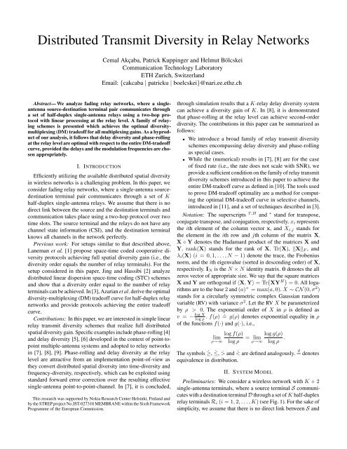
Preliminaries: We consider a wireless network with K + 2
single-antenna terminals, where a source terminal S communicates
with a destination terminal D through a set of K half-duplex
relay terminals R i (i = 1, 2, . . . , K) (see Fig. 1). For the sake of
simplicity, we assume that there is no direct link between S and

{f i}
S
source
R 1
R 2
· · ·
{h i}
D
destination
where z (when conditioned on h) is a circularly symmetric
Gaussian noise vector with E{z|h} = 0 and E{zz H |h} =
I N . In the remainder of the paper, we shall √be interested in
ρ
the ρ → ∞ case where
≈ ρ
1+‖h‖
. With
2
H eff =
√
ρ
1+||h|| 2
K∑
h i f i G i , we can now rewrite the inputoutput
relation (3) as
√
1+ρ(1+‖h‖ 2 )
i=1
R K
relay terminals
y = H eff x + z. (4)
Fig. 1.
Two-hop relay network with K single-antenna relay terminals.
D. The channels 1 S → R i , denoted as f i , and R i → D, denoted
as h i , (i = 1, 2, . . . , K), are i.i.d. CN (0, 1). We define the
column vectors f = [f 1 f 2 · · · f K ] T and h = [h 1 h 2 · · · h K ] T .
Communication takes place over two time slots. In the first
time slot, S transmits N symbols consecutively. The relay
terminals process the received length-N sequence using a linear
transformation and transmit the result during the second
time slot to D, while S remains silent. We assume that S and
the relay terminals do not have CSI, whereas D knows f i , h i
(i = 1, 2, . . . , K) perfectly. For simplicity, we further assume
perfect synchronization and ignore the impact of shadowing and
pathloss.
Signal model: The vectors x, r i , y ∈ C N represent the
N-dimensional transmitted symbol sequence, received symbol
sequence at R i , and received symbol sequence at D, respectively.
The vector r i is then given by
r i = √ ρf i x + w i , i = 1, 2, . . . , K (1)
where ρ denotes the average signal-to-noise ratio (SNR) (for
all links) and w i is the N-dimensional noise vector at R i , with
i.i.d. CN (0, 1) entries. The w i are independent across i as well.
We assume an i.i.d. Gaussian codebook with covariance matrix
R xx = E{xx H } = I N .
R i applies the unitary transformation G i according to
q i = G i r i and scales the result to meet the power constraint
E{‖q i ‖ 2 } = 1. This results in the overall input-output relation
y =
K∑
i=1
ρ
√ ρ + 1
h i f i G i x + ˜z (2)
where the effective noise term ˜z (when conditioned on h) is
circularly symmetric complex Gaussian ( with E{˜z|h} = 0 and
E{˜z˜z H |h} = N oI ′ N where N ′ o = 1 + ρ
ρ+1
). ‖h‖2
Since we will be interested in the mutual information under
the assumption that D knows all the channels in the network
perfectly, we can divide (2) by √ N ′ o to obtain the effective
input-output relation
y =
ρ
√
1 + ρ(1 + ‖h‖2 )
K∑
h i f i G i x + z (3)
i=1
1 A → B denotes the link between terminals A and B.
III. ACHIEVING THE OPTIMAL DIVERSITY MULTIPLEXING
TRADEOFF
Under the assumptions stated in the previous section, it follows
that the mutual information of the effective channel in (4) is given
by
I(y; x|H eff ) = 1
N−1
∑
log(1 + λ n (H eff H H
2N
eff)) (5)
n=0
where the factor 1/2 is due to the half-duplex constraint. We
shall next compute the optimal DM-tradeoff curve [10] for the
effective channel H eff and provide a sufficient condition on
the unitary matrices G i to achieve the entire tradeoff curve.
Following the framework in [10], we define a channel outage
event to occur if the mutual information does not support a target
data rate of R = r log ρ (b/s/Hz). The probability of outage at
multiplexing rate r and signal-to-noise ratio (SNR) ρ is then
P O (ρ, r) = P[I(y; x|H eff ) < r log ρ] . (6)
Directly analyzing (6) is challenging for the problem at hand as
closed-form expressions for the eigenvalue distribution of H eff
do not seem to be available. However, noting that
where
I(y; x|H eff ) ≤ I J (y; x|H eff ) (7)
I J (y; x|H eff ) = 1 2 log (
1 + 1 N
N−1
∑
n=0
= 1 2 log (1 + 1 N ‖H eff‖ 2 F
λ n (H eff H H eff)
)
)
, (8)
we can resort to a technique developed in [11] to show that
the DM-tradeoff corresponding to I J (y; x|H eff ) equals that
corresponding to I(y; x|H eff ). The significance of this result
lies in the fact that the quantity ‖H eff ‖ 2 F lends itself nicely to
analytical treatment.
In the following, we will need the Gramian matrix for the set
Q = {G 1 , G 2 . . . , G K } defined as
⎡
Tr ( )
G 1 G H 1 · · · Tr ( ) ⎤
G K G H 1
K = 1 Tr ( )
G 1 G H 2 · · · Tr ( )
G K G H 2
⎢
⎥
N ⎣ . . .
Tr ( )
G 1 G H K · · · Tr ( ⎦ . (9)
)
G K G H K
Our main result can now be summarized as follows.

Theorem 1: For the half-duplex relay channel in (4), the
optimal DM-tradeoff curve is given by
d(r) = K(1 − 2r) + , r ∈ [0, 1 ]. (10)
2
Any linear relay processing scheme Q = {G 1 , G 2 . . . , G K }
satisfying rank(K) = K achieves the entire DM-tradeoff curve.
Proof: See Appendix A.
Discussion: Theorem 1 shows that the DM-tradeoff properties
of the half-duplex relay channel in (4) are equal to the “cooperative
upper bound” (apart from the factor 1/2 loss, which is
due to the half-duplex constraint) corresponding to a system
with one transmit and K cooperating receive antennas. The lack
of cooperation and noise forwarding at the relay level, hence,
do not impact the DM-tradeoff behavior, provided the matrices
{G i } K i=1 are chosen such that rank(K) = K. Azarian et al.
[3] propose a protocol that achieves the optimal DM-tradeoff of
the amplify-and-forward half-duplex relay channel and attains
orthogonality between the relay transmissions by allowing only
one relay to transmit in any given time slot. Our results show that
there exists a whole family of linear relay processing schemes
that are DM-tradeoff optimal and that rank(K) = K is sufficient
to achieve tradeoff optimality. Another immediate conclusion
that can be drawn from Theorem 1 is the DM-tradeoff optimality
of cyclic delay diversity [7] and phase-rolling [8], [9] at the relay
level, provided the delays and modulation frequencies are chosen
appropriately. This can be seen by noting that the cyclic delay
diversity scheme [7] can be cast into our framework by setting
G i = P i where P i denotes the permutation matrix that when
applied to a vector x cyclically shifts the elements in x up by i
positions.With
{
N, for i = j
〈P i , P j 〉 =
0, for i ≠ j
the Gramian of Q is given by K = I K which upon application of
Theorem 1 concludes the argument. In the case of phase-rolling
[8], [9], we have
⎡
G i =
⎢
⎣
⎤
e jθi[0] 0 0
.
. ..
⎥
. ⎦
0 0 e jθi[N−1]
which, choosing the modulation frequencies θ i [n] = 2πn(i−1)
N
gives
{
N, for i = j,
〈G i , G j 〉 =
0, for i ≠ j
and hence rank(K) = K, concludes the argument. While the
(numerical) results in [7], [8] are for the r = 0 case, our analysis
reveals optimality of cyclic delay diversity and phase-rolling for
the entire tradeoff curve.
Numerical results: We illustrate our results numerically using
a network consisting of K = 4 relays. Fig. 2 shows the outage
probability (obtained through Monte Carlo simulation) as a
function of SNR for the cyclic delay diversity scheme with
K = I 4 and for four other linear relay processing schemes with
rank(K) = 1, 2, 3, and 4, respectively, and nonzero spread of
the positive eigenvalues of K. We observe that both the cyclic delay
diversity scheme and the scheme with rank(K) = 4 achieve
a diversity order of 4. However, the delay diversity scheme offers
slightly better performance indicating that orthogonality between
the G i improves performance. Moreover, the numerical results
suggest that the diversity order achieved by the other schemes
is given by rank(K). However, at this point, we do not have a
proof of the latter statement.
Outage Probability
10 0 C. delay diversity
Rank 4 scheme
Rank 3 scheme
10 !1
Rank 2 scheme
Rank 1 scheme
10 !2
10 !3
10 !4
10 !5
10 !6
0 5 10 15 20 25 30
SNR(dB)
Fig. 2. Outage Probability vs. SNR for a delay diversity scheme and for four
other schemes with different ranks.
IV. CONCLUSIONS
We introduced a family of linear relay processing schemes
achieving the optimal DM-tradeoff of half-duplex relay channels.
Cyclic delay diversity and phase-rolling were shown to be special
(DM-tradeoff optimal) cases. Our results can be readily extended
to account for the presence of a direct link between the source and
the destination terminals. The DM-tradeoff framework seems to
be too crude to distinguish between different full-rank schemes
suggesting that a finer analysis is needed to quantify the impact
of the eigenvalue spread of the Gramian matrix of the G i .
APPENDIX A
PROOF OF THEOREM 1
We start by noting that an upper bound on the DM-tradeoff
curve can be obtained by applying the broadcast cut-set bound
[12] to the network in Fig. 1 and evaluating the corresponding
DM-tradeoff. It is shown in [12], [13] that the broadcast cut
amounts to a point-to-point link with a single transmit and K
(cooperating) receive antennas. Taking into account the factor
1/2 loss due to the half-duplex nature of the relay terminals,
it follows from the results in [10] that the DM-tradeoff curve
corresponding to the network analyzed in this paper is upperbounded
by
d(r) ≤ K(1 − 2r) + , r ∈ [0, 1 2 ].
In the following, we shall show that this upper bound is achievable
despite the lack of cooperation at the relay terminals provided
the matrices G i are chosen such that rank(K) = K. We
start by noting that
P O (ρ, r) ≥ P[J ] = P[I J (y; x|H eff ) < r log ρ] (11)

and defining the event
J = {H eff |I J (y; x|H eff ) < r log ρ} (12)
as “Jensen outage”. Since
⎛
1
N ‖H eff‖ 2 ρ
K∑
F =
N(1 + ‖h‖ 2 ) Tr ⎝
=
ρ
1 + ‖h‖ 2 ˜h H K˜h,
i=1 j=1
⎞
K∑
(h i f i )(h ∗ j fj ∗ )G i G H ⎠
j
where ˜h = h ◦ f, it follows that
[ (
) ]
1
P[J ] = P
2 log 1 + ρ˜h H K˜h
1 + ‖h‖ 2 < r log ρ . (13)
In what follows, we write |h i | 2 = ρ −ui and |f i | 2 = ρ −vi
where u i and v i are RVs; the choice of this transformation
will become clear later. Further, we define the events A =
{u i , v i | u i > δ, v i > δ, i ∈ {1, 2, . . . , K}} and Ā = {u i| u i ≤
δ, i ∈ {1, 2, . . . , K}} ∪ {v i | v i ≤ δ, i ∈ {1, 2, . . . , K}} for a
fixed δ > 0 . Using the law of total probability, we can write
P[J ] = P[A] P[J |A] + P [ Ā ] P [ J |Ā] (14)
and bound P[J ] according to
P[A] P[J |A] ≤ P[J ] ≤ P[A] P[J |A] + P [ Ā ] (15)
P[A] P[J |A] ˙≤ P[J ] ˙≤ P[A] P[J |A] (16)
P[J |A] ˙≤ P[J ] ˙≤ P[J |A] (17)
where (16) follows from the definition of the u i and the v i ,
log P[Ā]
log ρ
their independence and by noting that lim = 0. The
ρ→∞
double inequality (17) results from P[A] = (1 − exp[−ρ −δ ]) K ,
lim
ρ→∞
log P[A]
log ρ
= −δK, and the fact that δ can be made arbitrarily
small. We have thus shown that P[J ] = . P[J |A]. Next, denoting
the minimum and maximum eigenvalue of K as λ min and λ max ,
respectively, we get the upper bound
[ ( 1
P[J |A] ˙≤ P
2 log 1 + ρ λ ) ]
min
1 + K ‖˜h‖ 2 < r log ρ (18)
[ (
) ]
1
= P
2 log 1 + ρ λ K∑
min
|f i | 2 |h i | 2 < r log ρ (19)
1 + K
i=1
[ (
) ]
1
= P
2 log 1 + λ K∑
min
ρ 1−vi−ui < r log ρ , (20)
1 + K
i=1
and the lower bound
[ 1
(
P[J |A] ˙≥ P
2 log 1 + ρλ max ‖˜h‖ 2) ]
< r log ρ
[ (
) ]
1
= P
2 log ∑
K
1 + ρλ max |f i | 2 |h i | 2 < r log ρ
i=1
[ (
) ]
1
= P
2 log ∑
K
1 + λ max ρ 1−vi−ui < r log ρ
i=1
(21)
(22)
(23)
where the key steps (18) and (21) follow from the Rayleigh-Ritz
∑
theorem [14] and the fact that 1 ≤ 1 + K ρ −ui ≤ 1 + K
for u i > 0 (i = 1, 2, . . . , K) and ρ > 1. Note that due to the
assumption rank(K) = K, we have λ min > 0. We define the
following events
i=1
{
}
B = u i , v i |max(1 − v i − u i ) > 0
i
{ ∣ ( ∣∣∣ 1
U = u i , v i
2 log 1 + λ minρ maxi(1−vi−ui) ) }
< r log ρ
1 + K
{ ∣ ∣∣∣ 1
(
L = u i , v i
2 log 1 + Kλ max ρ maxi(1−vi−ui)) }
< r log ρ
where the max is taken over i = 1, 2, . . . , K in all three cases.
With these definitions, we arrive at
P[L] ˙≤ P[J |A] ˙≤ P[U] (24)
P[L ∩ B] + P [ L ∩ ¯B ] ˙≤ P[J |A] ˙≤ P[U ∩ B] + P [ U ∩ ¯B ]
where (24) follows from
P[L ∩ B] ˙≤ P[J |A] ˙≤ P[U ∩ B] + P [ ¯B]
(25)
K∑
ρ 1−vi−ui ≤ Kρ maxi(1−vi−ui) (26)
i=1
K∑
ρ 1−vi−ui ≥ ρ maxi(1−vi−ui) (27)
i=1
and the RHS of (25) follows from conditioning with respect to
event B. Now we can expand P[U ∩ B] as
[
]
P[U ∩ B] = P 0 < max(1 − v i − u i ) < 2r + ɛ 1 (28)
i
(
( )) K
1
1
= 1 − √ K 1 √ (29)
ρ
1−2r−ɛ 1 ρ
1−2r−ɛ 1
.
= ρ −K(1−2r)+ (30)
log(
1+K
λ min
)
where ɛ 1 =
log ρ
and K 1 (·) is the first-order modified Bessel
function of the second kind. Eq. (29) follows from
[
]
P 0 < max(1 − v i − u i ) < 2r + ɛ 1
i
( [
]) K ( [
= P |f 1 | 2 |h 1 | 2 1
<
− P |f 1 | 2 |h 1 | 2 < 1 ]) K
ρ 1−2r−ɛ1 ρ
and using the fact that the pdf of the square root of the product
of two Rayleigh distributed RVs is given by v(x) = xK 0 (x) for
x > 0, where K 0 (·) is the zeroth-order modified Bessel function
[15]. The exponential equality in (30) is proved using a Taylor
series expansion of f(x) = 1 − xK 1 (x) around x = 0 and
invoking asymptotic properties of the logarithmic function [16].
Similarly, one can show that
P [ ¯B] =
(
1 − 1 √ ρ
K 1
( 1 √ρ
)) K
.=
0. (31)

To complete the proof, we need to establish that P[L ∩ B] has
the same exponential behavior in ρ as P[U ∩ B]. Using the same
arguments as in (28)-(30), it follows readily that
P[L ∩ B] = P[0 < max i (1 − v i − u i ) < 2r − ɛ 2 ] (32)
(
( )) K
1
= 1 − √
1
K 1 √
(33)
ρ 1−2r+ɛ 2
ρ 1−2r+ɛ 2
.
= ρ −K(1−2r)+ (34)
where ɛ 2 = log(Kλmax)
log ρ
. We have thus shown that
ρ −K(1−2r)+ ˙≤ P[J ] ˙≤ ρ −K(1−2r)+ (35)
and hence
P[J ] = P J (ρ, r)
.
= ρ −K(1−2r)+ , r ∈ [0, 1 ].
2
(36)
Since P J (ρ, r) ≤ P O (ρ, r) as a result of (7), and since the
outage probability is a lower bound to the error probability
achieved by any code [10], we have
P J (ρ, r) ≤ P O (ρ, r) ≤ P e (ρ, r). (37)
Following the approach proposed in [11], we complete the proof
of the theorem by identifying a code which has
.
P e (ρ, r) = P J (ρ, r)
and hence a DM-tradeoff curve which equals the “Jensen” DMtradeoff
curve derived above. We start by writing
P e (ρ, r) = P[J ] P[error|J ] + P [ error, J ¯ ] (38)
≤ P[J ] + P [ error, J ¯ ] . (39)
Next, we upper-bound P [ error, ¯ J ] through the union bound
P [ error, ¯ J ] ≤ ρ 2Nr P [ x 0 → x 1 , ¯ J ] (40)
where P [ x 0 → x 1 , J ¯ ] denotes the maximum pairwise error
probability (over all codeword pairs) for ML decoding, and
we used the fact that the codebook has ρ 2Nr codewords. With
∆x = x 1 − x 0 , we have
( ) ||H∆x||F
P[x 0 → x 1 |H eff = H] = Q √ (41)
2
[
]
≤ exp − ||H∆x||2 F
(42)
4
⎡
N∆x 2 min λ K∑
⎤
min ρ 1−vi−ui
˙≤ exp ⎢
⎣ − i=1 ⎥
4(1 + K) ⎦ (43)
where ∆x 2 min = min i ||∆x i || 2 , and (43) follows from noting
that ∆x is Gaussian and hence U∆x d = ∆x for unitary U,
from applying the Rayleigh-Ritz theorem, and from inserting
|h i | 2 = ρ −ui and |f i | 2 = ρ −vi into (42). Next, we have
P [ x 0 → x 1 , J ¯ ] (44)
⎧ ⎡
⎪⎨ N∆x 2 min λ K∑
⎤ ⎫
min ρ 1−vi−ui
≤ E exp ⎢
⎣
⎪⎩
− ⎪⎬
i=1 ⎥ ∣ ¯
4(1 + K) ⎦ J P [ ]
J ¯
⎪⎭
≤ exp
[− N∆x2 min λ minρ 2r ]
P [ ]
J ¯
4(1 + K)
(45)
where (45) follows since the event J ¯ requires that
K∑
ρ 1−vi−ui ≥ ρ 2r . Finally, inserting (45) into (40), and
i=1
using P [ ]
J ¯ ≤ 1, we get
P [ error, ¯ J ] ˙≤ ρ 2Nr exp
[− N∆x2 min λ minρ 2r
4(1 + K)
]
. (46)
Choosing the codebook such that ∆x min > 0 the proof is
complete since (46) decays exponentially fast in ρ for any r > 0
and hence
P e (ρ, r) ≤ P[J ] + P [ error, J ¯ ]
[
]
˙≤ P[J ] + ρ 2Nr N
exp −
4(1 + K) ∆x2 minλ min ρ 2r
˙≤ P[J ] = P J (ρ, r).
which combined with (37) yields the desired result.
REFERENCES
[1] J. N. Laneman and G. W. Wornell, “Distributed space-time-coded protocols
for exploiting cooperative diversity in wireless networks,” IEEE Trans. Inf.
Theory, vol. 49, no. 10, pp. 2415 – 2425, Oct. 2003.
[2] Y. Jing and B. Hassibi, “Distributed space-time coding in wireless relay
networks,” IEEE Trans. Wireless Comm., vol. 5, no. 12, Dec. 2006.
[3] K. Azarian, H. El Gamal, and P. Schniter, “On the achievable diversitymultiplexing
tradeoff in half-duplex cooperative channels,” IEEE Trans.
Inf. Theory, vol. 51, no. 12, pp. 4152–4172, Dec. 2005.
[4] J. Guey, M. P. Fitz, M. R. Bell, and W. Kuo, “Signal design for transmitter
diversity wireless communication systems over Rayleigh fading channels,”
in Proc. IEEE VTC, vol. 1, Atlanta, GA, Apr./May 1996, pp. 136–140.
[5] A. Wittneben, “Basestation modulation diversity for digital SIMULCAST,”
in Proc. IEEE VTC, St. Louis, MO, May 1991, pp. 848–853.
[6] N. Seshadri and J. H. Winters, “Two signaling schemes for improving
the error performance of frequency-division-duplex (FDD) transmission
systems using transmitter antenna diversity,” Int. J. Wireless Information
Networks, vol. 1, pp. 49–60, Jan. 1994.
[7] S. B. Slimane and A. Osseiran, “Relay communication with delay diversity
for future communication systems,” in Proc. IEEE Vehicular Technology
Conference, Sept. 2006.
[8] I. Hammerström, M. Kuhn, and A. Wittneben, “Cooperative diversity by
relay phase rotations in block fading environments,” in Proc. Fifth IEEE
Workshop on Signal Processing Advances in Wireless Communications,
SPAWC 2004, July 2004, pp. 293–297.
[9] P. Kuppinger, “Transformation of distributed spatial into temporal diversity
by relay phase rotations,” M.Sc. Thesis, Imperial College London, Sept.
2006.
[10] L. Zheng and D. N. C. Tse, “Diversity and multiplexing: A fundamental
tradeoff in multiple-antenna channels,” IEEE Trans. Inf. Theory, vol. 49,
no. 5, pp. 1073–1096, May 2003.
[11] P. Coronel and H. Bölcskei, “Diversity multiplexing tradeoff in selective
MIMO fading channels,” in Proc. IEEE ISIT, submitted, 2007.
[12] M. Gastpar and M. Vetterli, “On the capacity of large Gaussian relay
networks,” IEEE Trans. Inf. Theory, vol. 51, no. 3, pp. 765–779, March
2005.
[13] H. Bölcskei, R. U. Nabar, O. Oyman, and A. J. Paulraj, “Capacity scaling
laws in MIMO relay networks,” IEEE Trans. Wireless Comm., vol. 5, no. 6,
pp. 1433–1444, Jun. 2006.
[14] R. A. Horn and C. R. Johnson, Matrix Analysis. New York, NY:
Cambridge Press, 1985.
[15] J. Salo, H. El-Sallabi, and P. Vainikainen, “The distribution of the product
of independent Rayleigh random variables,” IEEE Trans. Antennas and
Propagation, vol. 54, no. 2, pp. 639–643, Feb. 2006.
[16] M. Abramowitz and I. Stegun, Handbook of Mathematical Functions. New
York: Dover, 1965.