Quantum Field Theory (a few lectures)
Quantum Field Theory (a few lectures)
Quantum Field Theory (a few lectures)

You also want an ePaper? Increase the reach of your titles
YUMPU automatically turns print PDFs into web optimized ePapers that Google loves.
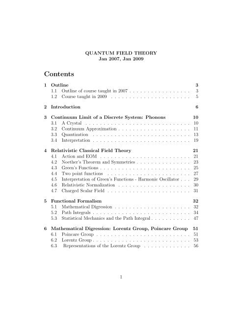
QUANTUM FIELD THEORY<br />
Jan 2007, Jan 2009<br />
Contents<br />
1 Outline 3<br />
1.1 Outline of course taught in 2007 . . . . . . . . . . . . . . . . . 3<br />
1.2 Course taught in 2009 . . . . . . . . . . . . . . . . . . . . . . 5<br />
2 Introduction 6<br />
3 Continuum Limit of a Discrete System: Phonons 10<br />
3.1 A Crystal . . . . . . . . . . . . . . . . . . . . . . . . . . . . . 10<br />
3.2 Continuum Approximation . . . . . . . . . . . . . . . . . . . . 11<br />
3.3 Quantization . . . . . . . . . . . . . . . . . . . . . . . . . . . 13<br />
3.4 Interpretation . . . . . . . . . . . . . . . . . . . . . . . . . . . 19<br />
4 Relativistic Classical <strong>Field</strong> <strong>Theory</strong> 21<br />
4.1 Action and EOM . . . . . . . . . . . . . . . . . . . . . . . . . 21<br />
4.2 Noether’s Theorem and Symmetries . . . . . . . . . . . . . . . 23<br />
4.3 Green’s Functions . . . . . . . . . . . . . . . . . . . . . . . . . 25<br />
4.4 Two point functions . . . . . . . . . . . . . . . . . . . . . . . 27<br />
4.5 Interpretation of Green’s Functions - Harmonic Oscillator . . . 29<br />
4.6 Relativistic Normalization . . . . . . . . . . . . . . . . . . . . 30<br />
4.7 Charged Scalar <strong>Field</strong> . . . . . . . . . . . . . . . . . . . . . . . 31<br />
5 Functional Formalism 32<br />
5.1 Mathematical Digression . . . . . . . . . . . . . . . . . . . . . 32<br />
5.2 Path Integrals . . . . . . . . . . . . . . . . . . . . . . . . . . . 34<br />
5.3 Statistical Mechanics and the Path Integral . . . . . . . . . . . 47<br />
6 Mathematical Digression: Lorentz Group, Poincare Group 51<br />
6.1 Poincare Group . . . . . . . . . . . . . . . . . . . . . . . . . . 51<br />
6.2 Lorentz Group . . . . . . . . . . . . . . . . . . . . . . . . . . . 53<br />
6.3 Representations of the Lorentz Group . . . . . . . . . . . . . 56<br />
1
7 Dirac <strong>Field</strong> 61<br />
7.1 Classical Dirac Equation and Solutions . . . . . . . . . . . . . 61<br />
7.2 Various Properties of the solutions . . . . . . . . . . . . . . . 63<br />
7.3 Gamma Matrix Properties . . . . . . . . . . . . . . . . . . . . 64<br />
7.4 Quantization of the Dirac <strong>Field</strong> . . . . . . . . . . . . . . . . . 66<br />
7.5 Properties of spin 1 states . . . . . . . . . . . . . . . . . . . . 67<br />
2<br />
7.6 Green’s Function . . . . . . . . . . . . . . . . . . . . . . . . . 69<br />
8 Discrete Symmetries:C,P,T 70<br />
8.1 P, T, C in QFT: . . . . . . . . . . . . . . . . . . . . . . . . . 72<br />
9 Functional Formalism for <strong>Field</strong> Theories 74<br />
9.1 Interactions - Functional Formalism: Z[J] . . . . . . . . . . . . 75<br />
9.2 Perturbative Evaluation of Z λ [J] . . . . . . . . . . . . . . . . 77<br />
9.3 Green’s Functions . . . . . . . . . . . . . . . . . . . . . . . . . 78<br />
9.4 Feynman Diagrams and Rules . . . . . . . . . . . . . . . . . . 80<br />
10 Functional Formalism for Fermions 82<br />
10.1 Grassmann Calculus . . . . . . . . . . . . . . . . . . . . . . . 82<br />
10.2 Dirac Action . . . . . . . . . . . . . . . . . . . . . . . . . . . . 85<br />
10.3 Application: Yukawa Interaction . . . . . . . . . . . . . . . . . 86<br />
11 Application to Particle Physics:S-Matrix 87<br />
11.1 LSZ Reduction Formula . . . . . . . . . . . . . . . . . . . . . 93<br />
11.2 S Matrix element for φ 4 . . . . . . . . . . . . . . . . . . . . . 94<br />
11.3 Scattering Cross Section . . . . . . . . . . . . . . . . . . . . . 95<br />
12 Application to Critical Phenomena 99<br />
13 Loops 102<br />
14 Renormalization 110<br />
14.1 Philosophy . . . . . . . . . . . . . . . . . . . . . . . . . . . . . 110<br />
14.2 Systematic Procedure . . . . . . . . . . . . . . . . . . . . . . . 112<br />
14.3 Renormalizing φ 4 theory . . . . . . . . . . . . . . . . . . . . . 113<br />
15 Wilson’s Interpretation 117<br />
2
16 Renormalization Group 123<br />
16.1 β function and evolution of coupling . . . . . . . . . . . . . . 123<br />
16.2 Wilson’s Renormalization group, Universality in Critical Phenomena<br />
. . . . . . . . . . . . . . . . . . . . . . . . . . . . . . 125<br />
16.3 Callan-Symanzik Equation . . . . . . . . . . . . . . . . . . . . 131<br />
17 <strong>Quantum</strong> Electrodynamics 131<br />
17.1 Canonical Analysis . . . . . . . . . . . . . . . . . . . . . . . . 132<br />
17.2 Green’s Function and Functional Formalism . . . . . . . . . . 133<br />
17.3 Canonical Quantization . . . . . . . . . . . . . . . . . . . . . . 136<br />
17.4 Generating Functional for QED . . . . . . . . . . . . . . . . . 137<br />
17.5 Tree Level Processes . . . . . . . . . . . . . . . . . . . . . . . 139<br />
17.6 One Loop Diagrams, Renormalization, beta-function . . . . . 139<br />
17.6.1 One Loop Graphs . . . . . . . . . . . . . . . . . . . . . 140<br />
17.7 Ward Identities . . . . . . . . . . . . . . . . . . . . . . . . . . 140<br />
1 Outline<br />
1.1 Outline of course taught in 2007<br />
Part I:<br />
1. Introduction. Why field theory and some intuition<br />
2. Concrete example: Phonons in a crystal and the continuum limit<br />
→Students should now have a physical picture of <strong>Quantum</strong><br />
<strong>Field</strong> <strong>Theory</strong><br />
3. Relativistic Classical <strong>Field</strong> <strong>Theory</strong>, EOM, Noether charge etc<br />
4. Other aspects: Green’s fn. two point correlators, relativistic normalization<br />
of states etc<br />
5. Causality, commutators<br />
6. Complex scalar field<br />
→ Students now know all about free relativistic scalar field<br />
theory<br />
Part II:<br />
3
7. Mathematical digression: Lorentz Group and its reps.<br />
8. Dirac Equation, gamma matrices, Weyl, Majorana etc.<br />
9. Quantization of Dirac <strong>Field</strong><br />
10. C,P,T<br />
Part III:<br />
11. Maxwell action, Gauge Invariance and Quantization, propagator..<br />
→Now students know all the usual free relativistiv QFT’s<br />
Part IV:<br />
12. Interactions - various kinds<br />
13. Perturbation theory, Interaction picture, Wick’s theorem<br />
14. Feynman Diagrams<br />
15. S-Matrix, Cross Section<br />
16. LSZ Reduction Formula, in states, out states etc.<br />
→ At this point students can in principle calculate S-matrices<br />
for all the usual QFT’s<br />
Part V:<br />
17. QED - some processes. tree level.<br />
Part VI:<br />
18. Functional formalism for free scalars, fermions and gauge theories,<br />
gauge fixing<br />
19. Fnl formalism for interacting theories. generating functional and Γ.<br />
20. One loop φ 4 theory.<br />
21. Renormalization: bare vs ren flds and parameters.<br />
Part VII:<br />
22. One loop QED - explicit calculations<br />
4
23. Ward Identities and BRS symmetry<br />
→ At this point the students knows how to do loop calculations<br />
and renormalize.<br />
1.2 Course taught in 2009<br />
The emphasis in 2009 was to teach a course that would be useful both for<br />
the high energy physicist as well as the low energy physicist. <strong>Field</strong> theory as<br />
used in particle physics is almost identical to what is used in for intance critical<br />
phenomena/ statistical physics. The functional integral (in D space +1<br />
time dimensions) after a Euclideanization (Wick rotation, which is done for<br />
calculational purposes anyway in particle physics) is the classical statistical<br />
mechanics partition function in D+1 space dimensions. The only difference<br />
is that in a particle physics courses the ostensible aim of calculating correlation<br />
functions is to calculate the S-matrix, whereas in statistical mechanics<br />
a major aim is to calculate critical exponents. Thus the entire package of<br />
field theory techniques is common to both disciplines. This however requires<br />
that we use the functional formalism. That was what was done in 2009. Two<br />
sections, one on S-matrix and one on critical phenomena, explains briefly the<br />
applications of the formalism to both disciplines.<br />
Note that Wick contractions and the usual operator method of perturbation<br />
theory in the interaction formalism was not done. If the Dirac theory<br />
and rep of Lorentz group are done away with, a couple of <strong>lectures</strong> on this<br />
can be included.<br />
1. Part 1<br />
Thus in 2009 the first two (out of three) parts of the course dealt with<br />
scalar field theory. The free theory was motivated by the crystal lattice<br />
example and the continuum limit taken. Canonical quantization<br />
was done. Green’s functions defined. Subsequently path integrals were<br />
introduced since the students had not done that. The functional formalism<br />
for field theories was developed. The connection to the usual<br />
Heisenberg and Schroedinger picture was made. The generating functional<br />
and the technique of Feynman diagrams for a perturbative evaluation<br />
was derived. The actual evaluation of integrals is done later.<br />
2. Part II<br />
5
A calculation of the scattering cross section is then given as an application<br />
to particle physics and as an application to critical pheneomena<br />
Landau theory for ferromagnetism with a scalar field (magnetization)<br />
as an order parameter is introduced. Critical exponents are defined<br />
and the role of ”mass” parameter in fld theory as the inverse correlation<br />
length in stat mech is explained.<br />
Loop integrals are evaluated and renormalization is described. The beta<br />
function and running coupling constant is explained. Wilson’s picture<br />
is given and the understanding of bare coupling and renormalized coupling<br />
as parameters defined at two widely different scales is explained.<br />
This gives an RG explanation for the process of renormalizing infinities<br />
by adding counterterms that the particle physicist is familiar with.<br />
Wilson’s idea of integrating out momentum shells to obtain a theory<br />
with a lower cutoff and a modified coupling constant is described. An<br />
explicit example of the free scalar field is given in some detail and the<br />
concept of relevant, irrelevant and marginal operators is explained in<br />
the context of this free scalar theory. The non trivial fixed point of φ 4<br />
theory in less than 4 dimensions is shown. (4-5 <strong>lectures</strong> were spent of<br />
these aspects of RG) Universality in critical phenomena is explained.<br />
3. Part III<br />
Electrodynamics. Gauge invariance and the Fadeev Popov procedure<br />
for gauge fixing is described. Photon propagator is derived. Canonical<br />
quantization in Coulomb gauge is done. Ward identities are introduced<br />
- using functional methods.<br />
One lecture on rep of Lorentz roup was given. Dirac theory. Green’s<br />
functions are defined. Quantization with anticommutators is introduced.<br />
Functional formalism form with Grassmann variables is defined<br />
and the generating functional is set up.<br />
Tree level processes in QED are calculated. One loop renormalization.<br />
beta function. Ward-Takahashi identitites.<br />
2 Introduction<br />
1. Introduction<br />
6
• Why field theory? ANS: Start with the example of electromagnetic<br />
phenomena. Classical electromagnetic phenomena is well<br />
described by the introduction of the concept of an electromagnetic<br />
field. E(x, ⃗ y, z, t), B(x, ⃗ y, z, t). There the introduction of<br />
the field allows you to do away with “action at a distance”. i.e.<br />
a charge acts on another charge through the medium of an electric<br />
field that it creates everywhere. Very useful. Makes it local.<br />
The existence of electromagnetic waves - prediction of Maxwellmakes<br />
the idea of a field more ’real’. It is hard to describe wave<br />
phenomena without the idea of a field pervading space.<br />
Other examples: whenever there is a continuous medium that has<br />
dynamical properties eg water, air, it is useful to introduce the<br />
idea of a field to describe properties of the material as a function<br />
of space and time. eg. pressure p(x, y, z, t), density ρ(x, y, z, t)<br />
..etc.<br />
The idea of a field in electromagnetism is a little different from<br />
the idea of a field in fluid mechanics. In the former we believe it<br />
to be an exact description. In the latter it is an approximation.<br />
But the techniques of classical field theory are applicable to both.<br />
But what about quantum field theory?<br />
It is now a fundamental idea and all fundamental entities in particle<br />
physics are described as fields. The application of quantum<br />
mechanics to particle physics requires quantum field theory.<br />
• Connection with Statistical Mechanics- If we Wick rotate<br />
t → −it we get a Euclidean theory that can be related to<br />
stat mech where becomes kT . This remarkable fact allows<br />
all the techniques and concepts of QFT to be used in understanding<br />
Critical Phenomena in Condensed matter systems. This connection<br />
is easiest to see in the ”feynman path integral” approach<br />
to field theory, (which is definitely the most flexible approach).<br />
Thus we can use the computational techniques of <strong>Quantum</strong> field<br />
theory to calculate correlation functions. In practice even in particle<br />
physics these calculations are done in Euclidean space (this is<br />
just the mathematical trick of analytic continuation). At the end<br />
of the day we rotate back to Minkowski space and interpret these<br />
in terms of scattering amplitudes. The same calculation can be<br />
done in studying critical phenomena where statistical fluctuations<br />
7
eplace quantum fluctuations and the field is an order parameter<br />
- an effective object rather than something fundamental.<br />
• Importance of space time continuum: Not really fundamental.<br />
can be thought of as a mathematical idealization. Useful<br />
because differential equations are understood better than difference<br />
equations. Thus even though we know that water is made<br />
up of discrete entitities - water molecules - we introduce the notion<br />
of ρ(x, y, z, t) (density) as if it is a continuous function. This<br />
is useful because in practice things are reasonably continuous in<br />
some approximation.<br />
We used to believe that space time is really a continuum - but<br />
nowadays it is not taken as sacroscanct - esp in theories of quantum<br />
gravity.<br />
• quantum versus classical: we believe that everything is quantum<br />
mecahnical. Therefore all dynamical variables should be<br />
treated as quantum mechanical - including the fundamental fields.<br />
These need not be true for effective fields - which may be described<br />
by classical mechanics. This means that after the problem<br />
has been treated quantum mecahnically the resultant theory is described<br />
by some convenient dynamical variables that obey some<br />
differential equations. These can be treated as classical. In practice<br />
we may write down these final equations directly by observing<br />
nature at macroscopic scales. we just assume that there is a fundamental<br />
quantum mechanical description from which these can<br />
be derived. Thus the elctromagnetic field is quantum mechanical.<br />
The density waves in air are classical.<br />
• particles versus fields: when a field is quantized we get discrete<br />
excitations of the field. These are photons. Thus field becomes<br />
an operator that creates photons out of the vacuum. The formalism<br />
thus allows particle production and destruction. Whenever<br />
these process are important - as in relativistic particle physics -<br />
field theory is useful. Ordinary quantum mechanics formalism is<br />
clumsy.<br />
• inasmuch as they are extremely useful to describe nature we can<br />
say that they are real (in the ontological sense) entities.<br />
2. Electromagnetic <strong>Field</strong>:<br />
8
• As a motivation for the formalism let us start with the familiar<br />
example of em - photons. Consider an em wave moving in the +z<br />
direction. ω = kc. Assume the el fld is in the x-direction.<br />
E x (z, t) = ae i(kz−ωt) + a ∗ e −i(kz−ωt)<br />
Intensity ∝ |a| 2 .It is an exptl fact that the number of photons ∝<br />
intensity.So treat a as a harmonic oscillator (annihilation) operator<br />
and then a ∗ a becomes the number operator on quantization.<br />
So interpretaion of a † is - creation operator - creates a photon. In<br />
this case this photon has wave number k. Thus if |0〉 is the ground<br />
state of the harmonic oscillator - which means no photons, then<br />
|1〉 = a † |0〉 is the state with one photon and |2〉 = a † a † |0〉 becomes<br />
a state with two photons. Thus the formalism allows you to deal<br />
with varying number of particles.<br />
• Relativistic quantum field theory is the way to do QM relativistically.Otherwise<br />
there are at least suerficially clashes between QM<br />
and causality.<br />
• The notion of an em field has implicit in it the notion of a space<br />
time continuum. Thus E(x, t) - here x, t are real numbers.This<br />
creates problems because it suggests that an em wave can have arbitrarily<br />
small wavelength and therefore arbitrarily high wavenumber.<br />
The photon then has arbitrarily high momentum and energy.<br />
Also one can fit an infinite number of standing waves in a cavity.<br />
All these “infinities” cause problems. So we tend to assume in the<br />
intermediate stages of the calculation that things are discrete and<br />
later take the “continuum limit”. This is subtle.<br />
• In order to illustrate the issues involved in the continuum approximation<br />
to a discrete system we will start with a discrete system<br />
and derive a continuum description. A crystal where the atoms<br />
vibrate about their mean position. These vibrational waves are<br />
the pressure waves and the corresponding particles obtained on<br />
quantizing them are called phonons. Just like photons from em<br />
waves.<br />
9
3 Continuum Limit of a Discrete System: Phonons<br />
3.1 A Crystal<br />
We start by studying a model of a crystal.<br />
conditions for simplicity. q 1 = q N+1 . 1<br />
Impose periodic boundary<br />
L = 1 N∑<br />
˙q i 2 − 1 2 2 ΣN i=1ν 2 (q i+1 − q i ) 2 (1)<br />
i=1<br />
ν is a constant that has dimensions of frequency. Eqn of Motion (EOM)<br />
∂L(t)<br />
∂q i (t) − d ∂L(t)<br />
dt ∂ ˙q i (t) = 0 (2)<br />
−ν 2 (q i+1 − q i ) + ν 2 (q i − q i−1 ) + ¨q i (3)<br />
¨q i = −ν 2 (2q i − q i+1 − q i−1 ) (4)<br />
Try: q m (t) = Q K (t)e imK - Plane wave<br />
¨Q K (t)e imK = −2ν 2 Q K (t)e imK (2sin 2 K 2 ) (5)<br />
¨Q K (t) = −4ν 2 sin 2 K 2 Q K(t) (6)<br />
The solution is:<br />
Q K (t) = Q K (0)e −iω Kt<br />
; (7)<br />
ω K = ±2νsin K 2<br />
Our normal mode solutions are q m (t) = Q K (0)e −iω Kt e imK (8)<br />
1 Some redefinitions of variables have been done that are illustrated by the single harmonic<br />
oscillator Lagrangian. If we start with L = 1 2 mẊ2 − 1 2 kX2 and define √ mX = q,<br />
we get 1 2 ( ˙q2 − k m X2 ) = 1 2 ( ˙q2 − ν 2 q 2 )<br />
10
Allowed values of K will be fixed by boundary condns (bc).<br />
Let N be total no.Since q N+1 = q 1 , we must have e iNK = 1. So<br />
K = ± 2πn<br />
N<br />
. with n = 0, 1, ..N − 1. Step size is 2π . As N → ∞, K becomes continuous.<br />
N<br />
If a is the lattice spacing between atoms and L is the length of the crystal,<br />
then N = L.<br />
a<br />
K = 2πna<br />
L<br />
= ka = 2π λ a<br />
Since ma denotes a position, we can let ma = x.<br />
The normal mode solutions look like:<br />
We can then write:<br />
q m (t) = Q K (0)e<br />
2πn<br />
i( L<br />
)(ma) e −iω kt = e ikx e −iω kt<br />
q(x, t) = Q(k)e i(kx−ω kt)<br />
These are sound waves in the solid crystal. ω k = 2νsin ka<br />
2<br />
Finally, by linearity the final solution is a superposition:<br />
q(x, t) = ∑ k<br />
Q k e i(kx−ω kt) + cc (9)<br />
Since q(x, t) is real, we must add cc.<br />
3.2 Continuum Approximation<br />
• From a distance we don’t see the graininess of a crystalline solid.<br />
If a is very small , i.e. a
•<br />
q i+1 − q i = q(x + a) − q(x) ≈ a ∂q<br />
∂x<br />
Let us adopt the following convention for interpolating between two<br />
lattice points: any function F (x) that has the value F (ma) at x = ma<br />
and F ((m + 1)a) at x = (m + 1)a, keeps the value F (ma) for ma ≤<br />
x < (m + 1)a. (Step approximation). Then<br />
1<br />
lim<br />
a→0 a<br />
⇒<br />
∫ x+a<br />
x<br />
N∑<br />
F (ma) = 1 a<br />
m=1<br />
Thus we see that ∫ dx = a ∑ i . Also<br />
∑ ∂<br />
(q j ) = ∑ ∂q<br />
i i<br />
i<br />
dxF (x) = F (ma)<br />
∫ L<br />
0<br />
dxF (x)<br />
δ ij = 1 (10)<br />
Letting ia = x and ja = y, so that q i = q(x) and q j = q(y) and also<br />
δ(x − y) = 1 a δ ij<br />
because<br />
we see that<br />
a ∑ i<br />
∫<br />
∫<br />
1 ∂<br />
(q j ) =<br />
a ∂q i<br />
dx δ(x − y) = a ∑ i<br />
dx<br />
∫<br />
δ<br />
δq(x) q(y) =<br />
1<br />
a δ ij = 1<br />
dx δ(x − y) = 1<br />
from which we also get the relation between the functional derivative<br />
and ordinary derivative. Now write action in terms of q(x).<br />
∫<br />
1 L<br />
2a [<br />
0<br />
= 1 ∫ L<br />
2a [<br />
dx ( ˙q(x) 2 − ν 2 a 2 ( ∂q<br />
∂x )2 )]<br />
0<br />
dx ( ˙q(x) 2 − c 2 ( ∂q<br />
∂x )2 )]<br />
12
• The last step is to redefine the dynamical variable q to get rid of the<br />
negative power of a in front. Let φ(x) = √ 1<br />
a<br />
q(x). We get<br />
= 1 2 [ ∫ L<br />
0<br />
dx ( ˙φ(x) 2 − c 2 ( ∂φ<br />
∂x )2 )]<br />
This last step involving defining a rescaled field variable is called in<br />
technical jargon “wave function renormalization” or ”field renormalization”.<br />
• EOM: δS = ∂2 φ<br />
− c 2 ∂2 φ<br />
= 0<br />
δφ ∂t 2 ∂x 2<br />
• There can be many discrete versions for the same continuum version.<br />
Try adding (2q i − (q i+1 + q i−1 )) 2 to the crystal action. Does the continuum<br />
limit change? This is the issue of “universality” in the theory of<br />
critical phenomena. More on this later.<br />
3.3 Quantization<br />
• Step 1: Write as a sum of decoupled HO<br />
• Step 2 “Quantize” each mode<br />
• Step 3: Superpose “quantum” normal modes to get “quantum” field.<br />
• Step 4: take a → 0 and L → ∞ limits.<br />
Preliminary Simple Harmonic Oscillator:<br />
Classical:<br />
L = 1 2ẋ2 − 1 2 ω2 x 2<br />
H = 1 2 p2 + 1 2 ω2 x 2<br />
x(t) = Asin ωt + Bcos ωt<br />
x(0) = B ; ẋ(0) = ωA.<br />
So x(t) = p(0) sin ωt + x(0)cos ωt ω<br />
13
This can be written as:<br />
1 { [ √ ωx(0) − i p(0) √ ω<br />
√ √ ]<br />
2ω 2<br />
} {{ }<br />
a ∗<br />
e iωt + [√ ωx(0) + i p(0) √ ω<br />
√ ] 2<br />
} {{ }<br />
a<br />
e −iωt}<br />
Thus x(t) = 1 √<br />
2ω<br />
[<br />
a ∗ (0)e iωt + ae −iωt] ≡ 1 √<br />
2ω<br />
[a ∗ (t) + a(t)]<br />
Also p = ẋ and<br />
H = ωa ∗ a<br />
√ <strong>Quantum</strong> √ HO: Quantize [x, p] = i ⇒ [a, a † ] = Rescale a, a †<br />
a, a † to get [a, a † ] = 1.<br />
→<br />
Also H = 1 2 ω(aa† + a † a) = ωa † a + 1ω ≡ (N + 1 )ω. N is called the<br />
2 2<br />
number operator.<br />
————————————————————————–<br />
Digression: Schroedinger Formalism and Heisenberg Formalism<br />
In S.. formalism time dependence is in the wave function. In H.. formalism<br />
it is in the operator.<br />
Schroedinger Picture<br />
x, p satisfy the usual comm. relns. there is no reference to time. If we<br />
work in the x basis, we have wave functions ψ(x, t) on which p acts as −i ∂<br />
∂x .<br />
ψ evolves in time as |ψ, t〉 = e −iHt |ψ, 0〉.<br />
Heisenberg Picture The time dependence is in the operator.<br />
Time evolution:<br />
i ∂O<br />
∂t<br />
= [O, H]<br />
- heisenberg eqns.<br />
Thus a † (t) = e iωt a(0) follows from this. In general O(t) = e iHt O(0)e −iHt .<br />
Thus the “equal time commutation relations” hold, if they hold at t = 0. i.e<br />
[x(t), p(t)] = i, [a(t), a † (t)] = 1<br />
Connection between the two:<br />
14
|ψ, t〉 S = e −iHt |ψ, 0〉 S = e −iHt |ψ〉 H<br />
Thus at t = 0 the Heisenberg and Schroedinger states are the same. Also<br />
S〈ψ, t|O S |ψ, t〉 S = S 〈ψ, 0|e iHt O S e −iHt |ψ, 0〉 S = H 〈ψ|e iHt O H (0)e −iHt |ψ〉 H = H 〈ψ|O H (t)|ψ〉 H<br />
O H (t) = e iHt O S e −iHt .<br />
End of digression<br />
————————————————————————-<br />
Now we can perform the four steps of quantization.<br />
• Step 1: Normal mode decomposition:<br />
q m (t) =<br />
2π∑<br />
K=0<br />
Q K (0)e −iω Kt e imK + c.c<br />
K = 2πn<br />
N .K max = 2π (when n = N).<br />
One finds that (Using ∑ m eim(K+K′) = δ K,−K ′)<br />
∑<br />
qm(t) 2 = N<br />
m<br />
n=+ 1 2 N ∑<br />
n=− 1 2 N {<br />
− ω<br />
2<br />
K [Q K Q −K + Q ∗ KQ ∗ −K] + ω 2 K[Q K Q ∗ K + c.c] }<br />
The factor N comes from the number of sites.<br />
Similarly one finds that<br />
ν 2 ∑ m<br />
n=+<br />
∑<br />
1 2 N<br />
(q m+1 −q m ) 2 = Nν 2<br />
n=− 1 2 N {<br />
(e iK −1)(e −iK −1)[Q K Q −K +Q ∗ KQ ∗ −K]<br />
+(e iK − 1)(e −iK − 1)[Q K Q ∗ K + c.c] }<br />
Using (e iK − 1)(e −iK − 1) = 4sin 2 K 2 ,<br />
ν 2 ∑ m<br />
(q m+1 −q m ) 2 = N<br />
n=+ 1 2 N ∑<br />
n=− 1 2 N ω 2 K<br />
{<br />
[QK Q −K +Q ∗ KQ ∗ −K]+[Q K Q ∗ K +c.c] }<br />
15
Adding we get:<br />
1<br />
2<br />
∑<br />
q m (t) 2 + 1 ∑ 2 ν2 m<br />
m<br />
(q m+1 − q m ) 2 = N ∑ K<br />
ω 2 K[Q K Q ∗ K + c.c]<br />
Finally rescaling :<br />
a K = √ N2ω K Q K<br />
we get<br />
H = 1 ∑<br />
ω K [a K a ∗ K + c.c.]<br />
2<br />
K<br />
q M (t) = √ 1<br />
n=+<br />
∑<br />
1 2 N<br />
√ [a K (t)e imK +cc] ; p m (t) = ˙q m (t) (11)<br />
N 2ωK<br />
n=− 1 2 N 1<br />
END OF STEP 1.<br />
• Step 2: Quantize each mode:<br />
a K (0) → √ a K<br />
a ∗ K(0) → √ a † K<br />
. [a K , a † K ] = δ K,K ′ ; H = ∑ K<br />
ω K (a K a † K + a† K a K)<br />
(IMP: Zero point energy = ∞ (as N → ∞)!!!)<br />
END of STEP 2<br />
• Step 3: Superpose:<br />
Calculate [q m (0), p m ′(0)] using the com relns of a, a † and eqn (11) and<br />
also using ∑ K ei(m−m′ )K = Nδ m,m ′ we get [q m , p m ′] = iδ m,m ′<br />
and other commutators [q, q]; [p, p] = 0.<br />
16
Using time evolution one gets [q m (t), p m ′(t)] = iδ m,m ′<br />
Equal Time Commutator (ETC) of QFT.<br />
END of STEP 3.<br />
Summary of what has been done so far: We start off with q m which<br />
is the displacement of an individual atom of the crystal. There are<br />
N of these. We could just demand that q m , p m have the usual comm<br />
reln. But instead we preferred to first separate into normal modes.<br />
The amplitude of a normal mode (travelling wave with a definite<br />
wave number) is our new position coordinate. There are N such modes<br />
and thus N of these coordinates. (So either way we have N dynamical<br />
variables and their conjugate momenta.) It has the advantage that it<br />
has the dynamics of a harmonic oscillator, which we can easily quantize.<br />
We prefer to work with creation and annihilation operators for this<br />
harmonic oscillator rather than its position and momentum. These are<br />
a K , a † K . This is then quantized. When we work our way back to q m, p m<br />
we find that they also obey the standard comm relns.<br />
Interpretation of q m is easy. Interpretation of a † K<br />
- creates an excitation<br />
corresponding to a wave with definite wave number. Collective mode.<br />
The wave is the sound wave and these discrete excitations ae phonons.<br />
This is the usual particle - wave duality of QM. Analog of this for EM<br />
is a photon.<br />
All that is left is to take the continuum limit, a → 0<br />
Exercise:1. Understand why ω K → 0 as K → 0 2. What would<br />
happen if we add a term 1 2 µ ∑ m q2 m to H of the crystal? What would<br />
this represent physically?<br />
• Step 4: Continuum Limit:<br />
Let a → 0 and L → ∞.<br />
We defined φ(x, t) = 1 √ a<br />
q(x, t) = 1 √ a<br />
q m (t) with x = ma.<br />
Π(x, t) = 1 √ a<br />
p(x, t) = 1 √ a<br />
p m (t) = 1 √ a ˙q m (t) = ˙φ(x, t) =<br />
Then<br />
δL<br />
δ ˙φ(x,t)<br />
Define<br />
[φ(x, t), Π(x ′ , t)] = 1 a [q m(t), p m ′(t)] = 1 a δ m,m ′<br />
17
What is lim a→0<br />
1<br />
a δ m,m ′?<br />
1<br />
lim<br />
a→0 a δ m,m ′ = 0, m ≠ m′<br />
= ∞, m = m ′<br />
= δ(x − x ′ )<br />
Check: Using ∫ dx δ(x − x ′ ) = a ∑ m<br />
δ m,m ′<br />
a<br />
= 1 We see thus that<br />
[φ(x, t), Π(x ′ , t)] = δ(x − x ′ )<br />
Now go to momentum space:<br />
φ(x, t) = √ 1 q m (t) = 1 ∑ 1<br />
√ √ [a K e imK + a †<br />
a<br />
K<br />
Na e−imK ]<br />
2ωK<br />
K<br />
Use K=2πn<br />
N , k = K a = 2πn<br />
L and also ∆k = 2π L ⇒ ∑ K = ∑ k = L ∫ π a<br />
−π<br />
a<br />
dk<br />
2π<br />
φ(x, t) = √ 1 L 1 ∫ π<br />
a<br />
√<br />
L 2ωK<br />
−π<br />
a<br />
dk<br />
2π [a Ke imK + a † K e−imK ]<br />
Finally let a K<br />
√<br />
L = a(k) , a<br />
†<br />
K√<br />
L = a † (k)<br />
We get [a(k), a † (k ′ )] = Lδ K,K ′. lim L→∞ Lδ K,K ′ = cδ(k − k ′ ) . For some<br />
c. ∫ ∑<br />
dk cδ(k − k ′ ) = 2π L k Lδ k,k ′ = 2π So ⇒ c = 2π. Thus<br />
we get [a(k), a † (k ′ )] = 2πδ(k − k ′ )<br />
φ(x, t) = √ 1 ∫ π<br />
a<br />
2ωk<br />
−π<br />
a<br />
dk<br />
2π (a(k, t)eikx + a † (k, t)e −ikx )<br />
18
End of Step 4<br />
= √ 1 ∫ π<br />
a<br />
2ωk<br />
3.4 Interpretation<br />
−π<br />
a<br />
dk<br />
2π (a(k)e−iωt+ikx + a † (k)e iωt−ikx ) (12)<br />
• We have a quantum theory of a crystal. We also have the continuuum<br />
limit of this. This gives us a “<strong>Quantum</strong> <strong>Field</strong> <strong>Theory</strong>”.<br />
• The physical interpretation for the various objects was also given.<br />
φ(x, t) is a field whose value gives the displacement of the atom. a(k) †<br />
is the creation operator for the harmonic oscillator labelled by the wave<br />
number k. These are normal modes of the original system. Because it<br />
is quantized we have discrete amounts of excitations in each mode. We<br />
call these particles.<br />
• Thus let |0〉 p be the ground state of the harmonic oscillator asssociated<br />
with wave number p. Then a † (p)|0〉 p ≡ |1〉 p is a state with one “particle”<br />
with wave number p (or momentum p). a † (p)a † (p)|0〉 p is a state<br />
with two particles. The HO is in it’s second excited state.<br />
• The state |1〉 p is what in ordinary QM we call |p〉 - a momentum<br />
eigenstate for the given particle. It’s wave function is proportional<br />
to e ikx−iωkt . What about |2〉 p ? It describes two particles. In ordinary<br />
QM we would introduce two coordinates and two momenta and label<br />
the wave functions as ψ(x 1 , x 2 ) or the kets as |p 1 , p 2 〉 or |x 1 , x 2 〉 etc. In<br />
this notation the state |2〉 p is |p, p〉. Note that both momenta are the<br />
same.<br />
• If we want particles with different momenta, we have to consider two<br />
different normal modes and thus two different HO’s. Thus we consider<br />
the state |0, 0〉 p1 ,p 2<br />
≡ |0〉 p1 ⊗ |0〉 p2 in the direct product Hilbert<br />
Space - which is the ground state of the combined system. Then<br />
a † (p 1 )a † (p 2 )|0, 0〉 p1 ,p 2<br />
≡ a † (p 1 )|0〉 p1 ⊗ a † (p 2 )|0〉 p2 = |1, 1〉 p1 ,p 2<br />
• Note an important difference with ordinary QM. The state a † (p)a † (p) =<br />
√<br />
2|2〉p is a two particle state. In field theory it is in the Hilbert space<br />
of one HO. Whereas |1, 1〉 p1 ,p 2<br />
(also a two particle state) is in a direct<br />
19
product Hilbert space of two HO’s. In ordinary QM both these states<br />
belong to the direct product Hilbert space (of two particles).<br />
• Thus in field theory the state |n〉 p is in the Hilbert space of one HO<br />
labelled by the wave number p, whereas in ordinary QM it would be in<br />
the direct product Hilbert space of n particles: |p〉 ⊗ |p〉 ⊗ |p〉 ⊗ ...|p〉.<br />
} {{ }<br />
n times<br />
Direct product space enters in field theory when we consider different<br />
wavenumbers, because there is one HO for each wave number. Thus if<br />
all n particles have different momenta, then we would be in the direct<br />
product space: |1〉 p1 ⊗ |1〉 p2 ⊗ .....|1〉 pn would be the state |p 1 , p 2 , ...., p n 〉<br />
in ordinary QM.<br />
• Consider the discrete space where there are N possible wavenumbers<br />
and hence N oscillators. The ground state of this system is<br />
|0〉 ≡ |0〉 −N<br />
2<br />
⊗ |0〉 −N−1<br />
2<br />
⊗ ......|0〉 N−1<br />
2<br />
⊗ |0〉 N<br />
2<br />
This state is annihilated by all the operators a K , ∀K i.e. a K |0〉 = 0.<br />
Then<br />
a † K |0〉 = |0〉 −N 2<br />
⊗ |0〉 −N−1<br />
2<br />
⊗ ...|1〉 K ⊗ ...|0〉 N−1<br />
2<br />
⊗ |0〉 N<br />
2<br />
we can use the label |K〉 for this state. It describes a phonon with wave<br />
number K.<br />
All the excitations of the system (with arbitrarily large number of particles)<br />
belong to the direct product Hilbert space of these N HO’s. This<br />
is called the Fock Space.<br />
• Now we can go back and see what φ(x, t) is precisely. It satisfies (using<br />
the mode expansion for φ and the properties of a’s:<br />
〈0|φ(x, t)|p〉 = 〈0|φ(x, t)a † (p)|0〉 = 1 √ 2ωp<br />
e −iωt+ikx<br />
Thus we can say that φ(x, t) is an operator that annihilates a particle at<br />
time t and position x. Thus φ † (x, t) creates a particle at x, t. φ(x, t) † |0〉<br />
is a state with a particle at x, t. It undergoes the usual time evolution<br />
20
given by the Schroedinger equation. In the Heisenberg formalism however<br />
the time dependence is in the operator. Thus the Schroedinger<br />
state of a particle at x is denoted by |x, t〉. In the Heisenberg picture<br />
we just take the state at time t = 0 and stay with that.<br />
Note that if φ is a real field then φ = φ † so φ can both create and<br />
annihilate particles at a point.<br />
• In the example of the crystal the field had a geometric interpretaion as<br />
a displacement of an atom. And the waves were thus sound waves and<br />
the particles are phonons. In particle physics for every particle that is<br />
observed in nature, we introduce a field. It usually does not have such<br />
a geometric interpretation. The only thing we care about is that the<br />
field operators create and destroy a particle.<br />
4 Relativistic Classical <strong>Field</strong> <strong>Theory</strong><br />
4.1 Action and EOM<br />
• Action: S = ∫ dt L = ∫ d 4 x L (L is Lagrangian, L is Lagrangian<br />
density)<br />
•<br />
∫<br />
=<br />
if δφ| B = 0.<br />
∫<br />
δS =<br />
d 4 ∂L<br />
x {<br />
∂φ(x, t) δφ + ∂L<br />
∂(∂ µ φ) δ(∂ µφ)} = 0<br />
d 4 ∂L<br />
x {<br />
∂φ(x, t) δφ − ∂ ∂L<br />
µ<br />
∂(∂ µ φ) δφ + ∂ ∂L<br />
µ[<br />
∂(∂ µ φ) δφ] }<br />
} {{ }<br />
Surface term<br />
⇒<br />
∂L<br />
∂φ(x, t) − ∂ ∂L<br />
µ<br />
∂(∂ µ φ) = 0<br />
These are the Lagrangian EOM. In “scalar field theory” L = − 1 2 ∂ µφ∂ µ φ<br />
then EOM is ∂ µ ∂ µ φ = 0 or ∂ 2 t φ−c 2 ∂ 2 i φ = 0. Relativistic wave equation.<br />
• Hamiltonian:<br />
H = ∑ m<br />
p m ˙q m − L(q m , ˙q m ) = ∑ m<br />
1<br />
2 p2 m(t) + 1 2 ν2 (q m+1 (t) − q m (t)) 2<br />
21
• Continuum limit:<br />
H = [ 1 2<br />
∫ dx<br />
a [p(x, t)2 + ν}{{}<br />
2 a 2 ∂q(x, t)<br />
( ) 2 ]<br />
∂x<br />
c 2<br />
Using p = √ aΠ, q = √ aφ we get<br />
= 1 ∫<br />
dx[Π 2 (x, t) + c 2 ∂φ(x, t)<br />
( ) 2<br />
2<br />
∂x<br />
In 3-space dim H = ∫ d 3 x [Π 2 (x, t) + |∇φ(x, t)| 2 ].<br />
where Π(x, t) =<br />
∫<br />
H =<br />
∂L<br />
∂ ˙φ(x,t)<br />
d 3 x [Π(x, t) ˙φ(x, t) − L(φ, ∂ µ φ)]<br />
• Heisenberg formalism operators are time dependent: O(t) = e iHt O(0)e −iHt .<br />
Thus formally the Hamiltonian is too but H(t) = H in the time independent<br />
case.<br />
• If L = − 1 2 ∂ µφ∂ µ φ − 1 2 m2 φ 2 then H will have an additional term :<br />
+ 1 2 m2 φ 2 . m can be shown to correspond to the mass of the particle.<br />
Study dispersion relation: find that E 2 = ⃗p.⃗p + m 2 c 4 .<br />
• Pts to emphasize: 1. Functional derivatives versus ordinary derivatives<br />
∫<br />
Thus<br />
dx 1 ∫<br />
∂q m<br />
=<br />
a ∂q n<br />
∑ ∂q m<br />
= ∑ ∂q<br />
m m ′<br />
m<br />
dx 1 ∫<br />
∂q(x)<br />
a ∂q(x ′ ) = } {{ }<br />
change of notation<br />
∫<br />
δ<br />
δq(x ′ )<br />
δ mm ′ = 1 (13)<br />
dx δq(x)<br />
δq(x ′ )<br />
∫<br />
=<br />
This can be obviously generalized:<br />
∫<br />
δ<br />
dx L(q(x)) = ∂L(x′ )<br />
δq(x ′ )<br />
∂q(x ′ )<br />
22<br />
dx δ(x − x ′ ) = 1<br />
(14)<br />
dx q(x) = 1 (15)<br />
(16)
2. H in Schr. form has no t. 3. Surface terms. 4. metric convention.<br />
5. = c = 1 convention.<br />
4.2 Noether’s Theorem and Symmetries<br />
Sometimes the action is invariant under global symmetries. In that case the<br />
equation of motion is left unchanged. Sometimes the Lagrangian is invariant,<br />
sometimes the Lagrangian density itself is invariant.<br />
• Infinitesimal symmetry transf: φ(x) → φ ′ (x) = φ(x) + δφ(x). e.g.:<br />
1. φ → φ + w. So δφ = w.<br />
2. If φ is complex, φ → e iω φ φ ∗ → e −iω φ ∗ . δφ = iωφ<br />
3. x µ → x µ − a µ = x ′µ and φ(x) → φ(x + a) = φ + a µ ∂ µ φ. Then<br />
δ a φ = a µ ∂ µ φ. Note: We take φ to be a scalar so that φ(x) =<br />
φ ′ (x ′ ) = φ ′ (x − a) or φ(x + a) = φ ′ (x). In this case the Lagrangian<br />
density is not invariant L → L + a µ ∂ µ L but the action is.<br />
• Noether’s theorem: for each such symmetry there is a conserved current<br />
and a conserved charge. To find the current a simple method is to<br />
consider a local variation :δ v φ where v(x) is some parameter. Thus<br />
δ v L = ∂L<br />
∂φ δ vφ +<br />
∂L<br />
∂(∂ µ φ) ∂ µ(δ v φ)<br />
Note that δ v ∂ µ φ ≡ ∂ µ δ v φ. Integrating by parts<br />
= [ ∂L<br />
∂φ − ∂ ∂L<br />
µ<br />
∂(∂ µ φ) ] ∂L<br />
δ v φ + ∂ µ [<br />
∂(∂<br />
} {{ }<br />
µ φ) δ vφ]<br />
= 0 by EOM<br />
= ∂ µ [vj µ ] = v∂ µ j µ + ∂ µ vj µ<br />
The action is invariant for constant v, then the total change in the<br />
Lagrangian density must be of the form ∂ µ [vN µ ]. Thus we find for<br />
constant v<br />
v∂ µ j µ = v∂ µ N µ<br />
So<br />
∂ µ J µ = 0]<br />
23
where J µ = j µ − N µ .<br />
This also defines j µ ∂L<br />
as the coefficient of ∂ µ v when we evaluate ∂ µ [ δ ∂(∂ µφ) vφ]<br />
. Note that the conservation of J µ is only after using EOM. Also note<br />
that if the Lagrangian density L is invariant then N µ is zero and in<br />
that case j µ is the conserved Noether current. If we define Q = ∫ d 3 xj 0<br />
then dQ = 0 is easy to see. This is the conserved Noether charge. In<br />
dt<br />
the examples above:<br />
1. j µ = ∂ µ φ<br />
2. j µ = i[φ∂ µ φ † − φ † ∂ µ φ]<br />
N is zero for the usual scalar Lagrangians.<br />
3. If scale invariant then δL = ∂ µ (ɛx µ L) = ∂ µ (a µ L) with a µ = ɛx µ .<br />
Dilatation Current in more detail: We are considering: x ′µ =<br />
1<br />
λ xµ We let λ = 1 + ɛ with ɛ 1, this means the new coordinates are smaller.<br />
This means the unit of length is bigger. System has shrunk. Momenta<br />
are stretched.)<br />
Let δ D φ(0) = dφ(0) - the field has a scaling dimension d. (If<br />
d > 0 it is like momentum.) Define RX = 1 X the finite abstract<br />
λ<br />
transformation. φ ′ (X ′ ) = φ ′ (RX) = Rφ(X) = λ d φ(x). Thus φ is<br />
not a scalar under this transf.<br />
φ ′ (x) = Rφ(R −1 x)<br />
φ ′ (x) − φ(x) = δ D φ = λ d φ(λx) − φ(x)<br />
δ D φ(x) = ɛ(d + x. ∂ )φ(x) (17)<br />
∂x<br />
Now consider a Lagrangian density L. If ∫ d 4 x L is to be invariant:<br />
4. In this case δL = a µ ∂ µ L = a ν ∂ µ [g ν µ L]. Thus The curren t N ν µ ≡<br />
g ν µ L corresponds to the transformation a ν . j ν µ = ∂L ∂ ∂(∂ µφ) νφ and<br />
thus<br />
J ν µ =<br />
∂L<br />
∂(∂ µ φ) ∂ νφ − g ν µ L<br />
Note that the role of the index ν is to label the transformation (a ν )<br />
and µ is the usual vector index associated with the current. For<br />
24
internal symmetries ν will be replaced by some internal index. The<br />
current defined above is in fact the energy momentum tensor<br />
T µ ν .<br />
Note that the charge associated with a 0 (time translation) is ∫ d 3 x T 0 0 =<br />
∫<br />
d 3 x [Π∂ t φ − L] = ∫ d 3 x H - Hamiltonian - as one would expect.<br />
4.3 Green’s Functions<br />
•<br />
L = − 1 2 ∂ µφ∂ µ φ − 1 2 m2 φ 2 + Jφ<br />
We have added a source - external force for a harmonic oscillator.<br />
EOM<br />
−∂ µ ∂ µ φ + m 2 φ = J<br />
Green’s fn G(x, x ′ )<br />
[−∂ µ ∂ µ + m 2 ]G(x, x ′ ) = δ 4 (x − x ′ )<br />
• Soln: Then<br />
∫<br />
φ(x) = φ 0 (x) +<br />
d 4 x ′ G(x − x ′ )J(x ′ )<br />
where φ 0 (x) is a soln of the hom eqn and satisfies the bc and then G<br />
goes to zero at the boundary. Eg. If bc is the value of φ(x, 0) then set<br />
φ 0 (x, 0) = φ(x, 0). Then G(x, x ′ ) should vanish at t = 0.<br />
• Momentum space:<br />
∫<br />
G(x, x ′ ) =<br />
∫<br />
δ 4 (x − x ′ ) =<br />
d 4 p<br />
(2π) 4 eip(x−x′) G(p)<br />
d 4 p<br />
(2π) 4 eip(x−x′ )<br />
⇒ [p µ p µ + m 2 ]G(p) = [−p 2 0 + p 2 i + m 2 ]G(p) = 1<br />
G(p) =<br />
1<br />
p 2 + m 2<br />
25
So<br />
∫<br />
G(x − x ′ ) =<br />
d 4 p e ip(x−x′ )<br />
∫<br />
(2π) 4 p 2 + m<br />
∫c<br />
= − dp 0<br />
2 2π<br />
d 3 p e −ip 0(x−x ′ ) 0 +ip i (x−x ′ ) i<br />
(2π) 3 (p 0 − E p )(p 0 + E p )<br />
Here E p = √ (p i ) 2 + m 2 .<br />
The contour c needs to be specified and will decide bc obeyed by G.<br />
1. C 1 Contour goes beneath both poles. If x 0 > x ′0 then convergence<br />
requires closing below so no poles are included. So G(x − x ′ ) = 0<br />
if x 0 > x ′0 . Propagates backwards in time. Hence G advanced .<br />
∫<br />
G adv (x−x ′ ) = iθ(x ′0 −x 0 )<br />
d 3 p<br />
(2π) 3 (e iEp(x−x′ ) 0 − e −iEp(x−x′ ) 0 )e ipi (x−x ′ ) i<br />
2E p<br />
2. C 2 Contour goes over both poles. Thus G is non zero only when<br />
x 0 > x ′0 . Thus we get G retarded .<br />
∫<br />
G ret (x−x ′ ) = iθ(x 0 −x ′0 )<br />
d 3 p<br />
(2π) 3 (e −iEp(x−x′ ) 0 − e iEp(x−x′ ) 0 )e ipi (x−x ′ ) i<br />
2E p<br />
Note that G ret and G adv are both real. G r is what is used in class<br />
mech. It is causal. G a answers the question of what should the<br />
fields be now in order to reach such and such state in the future.<br />
This is an unusual question in CM. We usually ask what is the<br />
state in the future given it is such and such now.<br />
3. C 3 Contour goes below −E p and above E p . This gives: x 0 > x ′0<br />
∫<br />
i<br />
d 3 −iE p (x − x ′ ) 0<br />
p 1 } {{ }<br />
e<br />
(2π) 3 +ve<br />
2E p<br />
+ip i (x−x ′ ) i<br />
and when x ′0 > x 0 we get<br />
∫<br />
i<br />
d 3 iE p (x − x ′ ) 0<br />
p 1 } {{ }<br />
e<br />
(2π) 3 −ve<br />
2E p<br />
+ip i (x−x ′ ) i<br />
26
Thus positive energy modes go forward in time and negative energy<br />
modes go backward in time. It can be written as:<br />
∫<br />
d 3 p 1<br />
G F eynman = i<br />
e −iEp|(x−x′ ) 0 |+ip i (x−x ′ ) i<br />
(2π) 3 2E p<br />
This contour prescription is equivalent to m 2 → m 2 − iɛ.<br />
This is the Green’s fn that one uses in QM.<br />
4.4 Two point functions<br />
• These Green functions of the classical theory can be related to “two<br />
point correlators” of QFT. (Expand on the idea of correlation functions<br />
- also Stat Mech connection.)<br />
Thus consider<br />
.<br />
∫<br />
φ(x, t) =<br />
∫<br />
φ(x ′ , t ′ ) =<br />
〈0|φ(x, t)φ(x ′ , t ′ )|0〉<br />
d 3 p 1<br />
√ [a<br />
(2π) 3 p e −iEpt+ip.x + a † pe +iEpt−ip.x ]<br />
2Ep<br />
d 3 q<br />
(2π) 3 1<br />
√<br />
2Eq<br />
[a q e −iEqt′ +iq.x ′ + a † qe +iEqt′ −iq.x ′ ]<br />
We get<br />
∫<br />
d 3 ∫<br />
p<br />
(2π) 3<br />
d 3 q<br />
(2π) 〈0| 1<br />
√ a 3 p e −iEpt+ip.x 1<br />
√ a † qe +iEqt′ −iq.x ′ |0〉<br />
2Ep 2Eq<br />
∫<br />
〈0|φ(x, t)φ(x ′ , t ′ )|0〉 =<br />
d 3 p 1<br />
e −iEp(t−t′ )+ip.(x−x ′) ≡ D(x − x ′ )<br />
(2π) 3 2E p<br />
Note that in this notation<br />
G ret (x−x ′ ) = iθ(t−t ′ )[D(x−x ′ )−D(x ′ −x)] = iθ(t−t ′ )〈0|[φ(x, t), φ(x ′ , t ′ )]|0〉<br />
27
• Similarly<br />
G F eynman (x − x ′ ) = i[θ(t − t ′ )D(x − x ′ ) + θ(t ′ − t)D(x ′ − x)]<br />
= i〈0|T (φ(x, t)φ(x ′ , t ′ ))|0〉<br />
where ”T ” stands for time ordering, i.e.<br />
time is to the right.<br />
the operator at the earlier<br />
• Finally consider 〈0|[φ(x, t), φ(x ′ , t ′ )]|0〉 when x, x ′ are spacelaike separated.<br />
In that case we can choose a frame where t = t ′ - D is Lorentz<br />
invariant. Therefore D(x − x ′ ) = D(x ′ − x) because one can perform a<br />
rotation, and D is only a fn of the distance. Therefore the commutatot<br />
vanishes for spacelike separation. ( If not spacelike one cannot relate<br />
x − x ′ and x ′ − x by a rotation/boost). This means φ(x) and φ(x ′ ) as<br />
operators can be simultaneously diagonalized. Measuring one doesn’t<br />
affect the other. This is required by causality. One can think of the<br />
influence going from x to x ′ - by particle propagation and anti particle<br />
(=particle going from x ′ to x), which cancel each other. <strong>Field</strong>s at<br />
spacelike separation are uncorrelated.<br />
• D(r) for spacelike r is ∫<br />
d 3 p<br />
(2π) 3 1<br />
2E p<br />
e ip.(x−x′ )<br />
This can be evaluated:<br />
∫ p 2 ∫<br />
dpd(cos θ) 1<br />
e iprcos θ =<br />
(2π) 3 2E p<br />
p 2 dp 1 e ipr − e −ipr<br />
(2π) 2 2E p ipr<br />
Using<br />
= − i<br />
4π 2 ∫ ∞<br />
−∞<br />
dp<br />
p<br />
r √ p 2 + m 2 eipr ≈ 1<br />
2π 2 r<br />
∫ ∞<br />
m<br />
p<br />
dp√ p2 − m 2 e−pr<br />
we get<br />
∫ ∞<br />
u<br />
xe −µx<br />
√<br />
x2 − u dx = uK 1(uµ) ≈ u√ 1 e −uµ<br />
2 uµ<br />
√ m<br />
r e−mr<br />
u → ∞<br />
≈ 1 r<br />
for large r.<br />
28
4.5 Interpretation of Green’s Functions - Harmonic<br />
Oscillator<br />
Consider the following equations for a HO<br />
d 2 y<br />
dt 2 + ω2 y = j(t) y(0) = y(T ) = 0 (18)<br />
This is the kind of bc that path integral requires. Consider different kinds<br />
off Green’s fns:<br />
• G Ret (t, t ′ ) : G Ret (t, t ′ ) = 0 ∀t < t ′<br />
• G Adv (t, t ′ ) : G Adv (t, t ′ ) = 0 ∀t > t ′<br />
• G F ey (t, t ′ ) : G F ey (0, t ′ ) = G(T, t ′ ) = 0 ∀t, t ′<br />
Let us construct these:<br />
G ret (t, t ′ ) = Asin ωt + Bcos ωt t > t ′<br />
G Ret (t, t ′ ) = 0 t < t ′ (19)<br />
Continuity requires that G(t ′ , t ′ ) = 0. Thus B = 0. A is fixed by ĠRet| t′ +ɛ<br />
t ′ −ɛ =<br />
1. So Aω = 1. A = 1 ω . Thus<br />
G Ret = 1 ω sinω(t − t′ )θ(t − t ′ ) (20)<br />
.<br />
G Adv can be obtained similarly. The continuity condn is G Adv (t ′ , t ′ ) = 0<br />
and ĠAdv(t, t ′ )| t′ +ɛ<br />
t ′ −ɛ<br />
= 1. This gives<br />
Let us work out G F ey :<br />
G Adv = − 1 ω sin ω(t − t′ )θ(t ′ − t)<br />
G F ey = A 1 sin ωt + B 1 cos ωt t > t ′<br />
= A 2 sin ωt + B 2 cos ωt t < t ′ (21)<br />
A 1 sin ωT + B 1 cos ωT = 0 and also B 2 = 0 are the bc’s. Continuity at<br />
t = t ′ gives:<br />
A 1 sin ωt ′ + B 1 cos ωt ′ = A 2 sin ωt ′<br />
29
and the remaining condition on derivatives is<br />
ωA 1 cos ωt ′ − ωB 1 sin ωt ′ − ωA 2 cos ωt ′ = 1<br />
We have three equations for three unknowns. Solve. Get<br />
G F =<br />
1<br />
sin ωT sin ω(t − T )sin ωt′ t > t ′<br />
1<br />
=<br />
sin ωT sin ω(t′ − T )sin ωt t < t ′ (22)<br />
This result will be useful later when we do path integrals.<br />
These Green’s function can be seen to be 0+1 dimensional versions of the<br />
field theory Green’s functions constructed earlier.<br />
4.6 Relativistic Normalization<br />
• δ 4 (p − q) is Lorentz scalar. δ 3 (p − q) is not but 2E p δ 3 (p − q) is where<br />
E p = + √ ⃗p.⃗p + m 2 .<br />
p ′ z = γ(p z + βE), E ′ = γ(E + βp z ).<br />
Use dp′ z<br />
dp z<br />
dp z δ(p z − q z ) = dp ′ zδ(p ′ z − q ′ z)<br />
δ(p z − q z ) = dp′ z<br />
dp z<br />
δ(p ′ z − q ′ z)<br />
= γ(1 + β dE<br />
dp z<br />
) = γ(1 + β pz<br />
) = E′<br />
E E<br />
• 〈q|p〉 = (2π) 3 δ 3 (p−q) in N.Rel QM. Define Rel 〈q|p〉 Rel = (2π) 3 2E p δ 3 (p−<br />
q)<br />
Thus |p〉 Rel = √ 2E p |p〉 NonRel = √ 2E p a † p|0〉<br />
• ∫ d 4 p is rel inv but not ∫ d 3 p. ∫ d 3 p<br />
2E p<br />
Thus<br />
∫<br />
1 =<br />
d 3 ∫<br />
p<br />
(2π) |p〉〈p| = 3<br />
is.<br />
d 3 p 1<br />
|p〉<br />
(2π) 3 rel<br />
2E p<br />
rel 〈p|<br />
Finally<br />
• ∫ d 3 p<br />
(2π) 3 2E p<br />
= ∫ d 4 p<br />
2πδ(p 2 − m 2 )|<br />
(2π) 4 p 0 >0 (Using 2xδ(x 2 − y 2 ) = δ(x − y))<br />
30
4.7 Charged Scalar <strong>Field</strong><br />
• Here φ = φ 1 + iφ 2 is complex, so one can just treat it as two real fields<br />
and be done. But typically the Lagrangian is invariant under φ → e iΛ φ<br />
and there is a conserved charge and current. Thus<br />
.<br />
L = 1 2 ∂ µφ ∗ ∂ µ φ − 1 2 m2 φ ∗ φ<br />
• The Noether current: J µ = i[φ∂ µ φ ∗ − φ ∗ ∂ µ φ]. Noether charge<br />
∫<br />
Q = d 3 x i[φ∂ t φ ∗ − φ ∗ ∂ t φ]<br />
∫<br />
=<br />
d 3 x [Πφ − Π ∗ φ ∗ ]<br />
• Mode expand:<br />
∫<br />
φ(x, t) =<br />
d 3 p<br />
(2π) 3 1<br />
√ 2ωp<br />
[a(p)e −iωpt+ip.x + b † (p)e iωpt−ip.x ]<br />
Note that coeff of +ve freq part is the annihilation operator. Since<br />
field is complex there is no reason for b = a. Thus φ destroys a type<br />
particles and creates b type particles.<br />
• One can check that<br />
∫<br />
d 3 p<br />
Q =<br />
(2π) 3 [a† (p)a(p) − b † (p)b(p)] = N a − N b<br />
Thus the two particles are of opposite charge, and same mass. Since<br />
they are part of the same field we can call them particles and antiparticles.<br />
•<br />
[φ(x), φ † (y)] = D(x − y) − D(y − x) = 0<br />
for spacelike separataion. One of the D’s is from a and the other is<br />
from b. One can think of it as a cancellation between particles going<br />
from y to x and anti particles from x to y. The mass thus has to be<br />
the same. In local cft particle is always accompanied by same mass<br />
antiparticle. If the fld is real, then particle = antiparticle.<br />
31
5 Functional Formalism<br />
This is a generalization of Feynman’s Path Integral formulation of quantum<br />
mechanics. Much more intuitive and conceptually simpler. Also more<br />
flexible. We will use the functional formalism for field theories. Begin with<br />
some mathematical preliminaries and then path integral formulation of QM.<br />
5.1 Mathematical Digression<br />
Gaussian Integrals<br />
1. ∫ ∞<br />
dx e − (x−x 0 )2<br />
2σ 2 = √ 2πσ 2<br />
−∞<br />
∫ ∞<br />
−∞<br />
dx (x − x 0 ) 2 e − (x−x 0 )2<br />
2σ 2 = √ 2πσ 2 σ 2<br />
σ 2 is the standard deviation and x 0 is the mean.<br />
From now on range of integration is assumed to (−∞, ∞) unless otherwise<br />
indicated.<br />
2. ∫<br />
dxe − 1 2 ax2 +jx =<br />
√<br />
2π<br />
a e 1 2 j 1 a j<br />
Trick: extremize the exponent wrt x: Get −ax + j = 0. x = j a .<br />
Plug this back into the exponent and get the answer. ”Semiclassical”<br />
approximation is the same as this.<br />
3.<br />
∫<br />
dx 1<br />
∫<br />
dx 2 e − 1 2 (a 1x 2 1 +a 2x 2 2 )+j 1x 1 +j 2 x 2<br />
=<br />
√<br />
2π<br />
a 1<br />
√<br />
2π<br />
a 2<br />
e 1 2 (j 1 1<br />
a 1<br />
j 1 +j 2<br />
1<br />
a 2<br />
j 2 )<br />
4. If A is a diagonal N × N matrix:<br />
⎛<br />
A =<br />
⎜<br />
⎝<br />
⎞<br />
a 1 0<br />
.<br />
.<br />
0 a N<br />
32<br />
⎟<br />
⎠ (23)
∫<br />
∫<br />
dx 1 ....<br />
dx N e − 1 2 xT Ax+j T x =<br />
(√ 2π) N<br />
√<br />
a1 a 2 ...a N<br />
e 1 2 jT (A −1 )j<br />
5. If A is a general real symmetric N × N matrix. Then let A = O T A D O<br />
be a diagonalization by an orthogonal matrix. Then x T Ax = y T D D y<br />
where y = Ox. The Jacobian of the tranformation of the integration<br />
measure [dy i ] = || ∂y i<br />
∂x j<br />
||[dx j ] is just Det O = 1. Thus we can use the<br />
previous formula and write:<br />
∫<br />
∫<br />
dx 1 ....<br />
6. Continuum Integrals<br />
∫<br />
I =<br />
dx N e − 1 2 xT Ax+j T x = (√ 2π) N<br />
Dx(t)e − 1 2<br />
Det 1 2 A e 1 2 jT (A −1 )j<br />
R<br />
dt<br />
R<br />
dt ′ x(t)A(t,t ′ )x(t ′ )+ R dt j(t)x(t)<br />
∫<br />
To make sense of this - discretize: t = jɛ and t ′ = kɛ. dt → ɛΣj<br />
x(t) = x(j) = x j and A(t, t ′ ) = A(j, k) = A j,k . x(t) becomes a column<br />
vector and A(t, t ′ ) becomes a matrix - very large N × N matrix. Take<br />
N → ∞ in the end as ɛ → 0.<br />
∫<br />
I =<br />
Π j dx j e − 1 2 ɛ2 Σ j,k x j A j,k x k +ɛΣ k J k x k<br />
where Σ k A −1<br />
j,k A k,l = δ j,l .<br />
= e 1 2 Σ j,kJ k (A −1 ) j,k J k<br />
√Det( 2π A )<br />
= e 1 2<br />
R R 1 dt dt<br />
ɛ 2 ′ J(t)(A −1 ) j= t<br />
ɛ<br />
,k= t′ J(t ′ )<br />
ɛ<br />
Define a A −1 (t, t ′ ) ≡ 1 A −1<br />
ɛ 2 j,k where t = jɛ and t′ = kɛ.<br />
√<br />
I = e 1 2<br />
R<br />
dt<br />
R<br />
dt ′ J(t)A −1 (t,t ′ )J(t ′ )<br />
Det( 2π A )<br />
Note also that<br />
Σ k A −1<br />
j,k A k,l = δ j,l<br />
33
∫ dt<br />
⇒ ɛ 2 ′<br />
ɛ A−1 (t, t ′ )A(t ′ , t”) = δ j,l<br />
where: jɛ = t, kɛ = t ′ , lɛ = t”. Thus<br />
∫<br />
dt ′ A −1 (t, t ′ )A(t ′ , t”) = δ j,l<br />
≡ δ(t − t”)<br />
ɛ<br />
7. Example: A(t, t ′ ) = A(t)δ(t − t ′ )<br />
So A j,k = A jδ j,k<br />
. A −1<br />
ɛ j,k = ɛ<br />
A j<br />
δ j,k . A −1 (t, t ′ ) = 1 A j<br />
δ j,k ɛ = δ(t−t′ )<br />
. Verify<br />
A(t)<br />
that ∫ A(t, t ′ )A −1 (t ′ , t”)dt = δ(t − t”) Thus<br />
∫<br />
√<br />
De − 1 R<br />
2 dt x 2 (t)A(t)+ R dt J(t)x(t) = e 1 R J(t) 2<br />
2 dt A(t)<br />
Det( 2π A )<br />
5.2 Path Integrals<br />
1. Instead of starting with a wave function one defines directly a probability<br />
amplitude for a particle to go from a point X i at time t i to a point<br />
X f at time t f . Call it K(X f , t f ; X i , t i ). Feynman defined the following<br />
formula for it: Motivation: double slit experiment.<br />
K(X f , t f ; X i , t i ) =<br />
∫ x(tf )=X f<br />
x(t i )=X i<br />
Dx(t) exp(+ i ∫ tf<br />
dtL(x(t), x(t)) ˙<br />
} {{ } t i<br />
sum over paths<br />
(24)<br />
Note that this is not the probability amplitude of a measurement, it is<br />
the probability amplitude of an event.<br />
2. Draw pictures and show classical limit. Principle of stationary phase.<br />
Derive Lagrange’s eqn.<br />
3. How do you actually calculate: What does Dx(t) mean? Divide t f − t i<br />
into N intervals ɛ = t j+1 − t j with t 0 = t i and t f = t N . Let x j = x(t j ).<br />
Then Dx(t) ≈ dx 1 dx 2 ....dx j ...dx N−1 There will in general a constant of<br />
proportionality (possibly infinite). Thus<br />
K(f, i) = K(X f , t f ; X i , t i ) = N<br />
∫ xN =X f<br />
x 0 =X i<br />
[dx 1 dx 2 ...dx N−1 ]e i S(f,i)<br />
Where S is the action and N is a normalization constant.<br />
34
4. The composition law K(a, b) = ∫ dx c K(b, c)K(c, a) : Draw figure. K<br />
is called Kernel. This can be iterated.<br />
5. Get<br />
∫<br />
K(X f , t f ; X i , t i ) =<br />
dx 1<br />
∫<br />
∫<br />
dx 2 ...<br />
dx N−1 K(f, N−1)K(N−1, N−2)...K(j+1, j)...K(1, i)<br />
(25)<br />
6. Do the integral ∫ dX i K(j + 1, j)K(j, j − 1)<br />
e i m<br />
<br />
2 [ x j+1 −x j<br />
ɛ<br />
] 2 + mɛ<br />
2 [ x j −x j−1<br />
ɛ ] 2<br />
=<br />
e im ɛ [(x j− x j+1 +x j−1<br />
2 ) 2 +( x j+1 −x j−1<br />
2 ) 2<br />
= √<br />
iɛ2π<br />
2m e i2ɛm<br />
2 ( x j+1 −x j−1<br />
) 2ɛ 2<br />
This is clearly proportional to K(j + 1, j − 1). The factor in square<br />
root is the normalization factor.<br />
Suppose the initial wave function corresponds to a particle with zero<br />
momentum. So ψ(X i , t i ) = √ 1<br />
V<br />
where V is the volume of space. After<br />
evolution the wave function is ψ(X f , t f ) = ∫ dX i K(X f , t f ; X i , t i ) √ 1<br />
V<br />
(see point 5 below). We know on physical grounds that ψ(X f , t f ) =<br />
√1<br />
V<br />
. Thus ∫ dX i K(X f , t f ; X i , t i ) = 1. Thus if we use the Gaussian<br />
normalization factor for each of the unit K’s , i.e. √ m<br />
final result √ m<br />
2π2ɛi e i2ɛm<br />
2 ( x j+1 −x j−1<br />
) 2ɛ 2<br />
which has the correct normalization.<br />
2πɛi<br />
, we get the<br />
Clearly this process can be iterated to replace 2ɛ by Nɛ = t f − t i . Thus<br />
√<br />
i(t<br />
m<br />
K(X f , t f ; X i , t i ) =<br />
2π(t f − t i )i e f −t i )m<br />
( (x f −x i )<br />
2<br />
(t f −t i ) )2 (26)<br />
35
7. Relation to wave functions - evolution operator.<br />
∫<br />
ψ(X f , t f ) = e −i R t f<br />
t Hdt i ψ(X i , t i ) =<br />
K(X f , t f ; X i , t i )ψ(X i , t i )dX i (27)<br />
8. Expansion of K(X f , t f ; X i , t i ) in terms of wave functions<br />
K(X f , t f ; X i , t i ) = ∑ n<br />
ψ n (X f )ψn(X ∗ i )e −i En(t f −t i )<br />
<br />
9. Derivation of Schroedinger’s eqn.<br />
Consider infinitesimal evolution from t to t + ɛ. The evolution operator<br />
is<br />
K(X f , t f ; X i , t i ) = ∫ x(t f )=X f<br />
x(t i )=X i<br />
We set t f = t i + ɛ to get<br />
ψ(X f , t i +ɛ) =<br />
∫ x(ti +ɛ)=X f<br />
x(t i )=X i<br />
∫<br />
Dx(t) exp(+ i tf<br />
} {{ }<br />
t i<br />
dtL(x(t), x(t)) ˙<br />
sum over paths<br />
Dx(t) exp( i ∫ ti +ɛ<br />
dtL(x(t), x(t))ψ(X ˙<br />
} {{ }<br />
i , t i )dX i<br />
t i<br />
sum over paths<br />
For infinitesimal evolution<br />
∫<br />
ψ(X f , t i + ɛ) = N<br />
e i m<br />
2 ɛ[ X f −X i<br />
ɛ<br />
] 2 ψ(X i , t i )dX i<br />
N is chosen so that the gaussian integral gives 1. bLHS is ψ(X f , t i ) +<br />
ɛ ∂ψ<br />
∂t i<br />
. Letting X f − X i = y and ψ(X f , t i ) = ψ(X i , t i ) + y ∂ψ + y2 ∂ 2 ψ<br />
(we<br />
∂y 2 ∂y 2<br />
get (linear term vanishes by symmetry)<br />
i ∂ψ = − 2 ∂ 2 ψ<br />
∂t i 2m ∂y 2<br />
(After multiplying by on both sides.) This is SE. QED.<br />
Note that K(X f , t f ; X i , t i ) satisfies SE. Also the bc lim tf →t i<br />
K(X f , t f ; X i , t i ) =<br />
δ(X f − X i ).<br />
36
10. getting semi classical energy, momentum. Using √ i(t<br />
m<br />
e f −t i )m<br />
( (X f −X i )<br />
2 (t f −t i ) )2<br />
2π(t f −t i )i<br />
we can understand semi classical limit : Change in phase wrt change in<br />
X f gives momentum and change wrt t f gives energy. Use K(X f , t f ; X i , t i )<br />
and study variation wrt X f . Prove that ∂ S ∂x cl = p.<br />
a)<br />
δS =<br />
S + δS =<br />
∫ tb<br />
t a<br />
b)Same thing for energy:<br />
∫ tb<br />
t a<br />
∫<br />
d<br />
dt [δx∂L ∂ẋ ]dt +<br />
S + δS =<br />
L(x + δx, ẋ + δẋ)dt<br />
δS = δx ∂L<br />
∂ẋ |t b<br />
tb<br />
∂S<br />
∂x b<br />
= ∂L<br />
∂ẋ |t b<br />
tb<br />
= P b<br />
∫ tb +δt b<br />
t a<br />
dt[eqn of motion]<br />
dtL(t, x ′ cl, ẋ ′ cl)<br />
x ′ is the modified classical solution. x ′ cl (t b + δt b ) = x cl (t b ) = x b .<br />
=<br />
S + δS =<br />
∫ tb<br />
t a<br />
δS = δt b L(x ′ cl, ẋ ′ cl) +<br />
∫ tb +δt b<br />
t a<br />
L(x ′ cl, ẋ ′ cl)dt<br />
L(x ′ cl, ẋ ′ cl) + δt b L(x ′ cl, ẋ ′ cl)<br />
∫ tb<br />
t a<br />
[L(x ′ cl, ẋ ′ cl) − L(x cl , ẋ cl )]dt<br />
The term in square brackets is after integrating by parts and using<br />
equations of motion δx cl<br />
δL<br />
δẋ .<br />
Using bc we get x ′ cl (t b) + ẋ ′ clδt b = x cl . So x ′ cl − x cl = −ẋ ′ clδt b . All this<br />
gives:<br />
δS = Lδt b +<br />
∫ tb<br />
dt[L(t, x<br />
′<br />
cl , ẋ ′ cl) − L(t, x cl , ẋ cl )<br />
37
= Lδt b + ∂L<br />
∂ẋ (x′ cl − x cl ) = Lδt b − pẋ cl δt b = −Eδt b .<br />
m<br />
c) Understand normalization: dx = P (b)dx.<br />
2πT<br />
mb<br />
T<br />
m(b + dx)<br />
< p <<br />
T<br />
Range of momentum dp = mdx . Thus the probability is of the form<br />
T<br />
1<br />
P (p)dp = const dp where const is<br />
11. Do the Gaussian slit - Feynman - and repeat results of wave packet<br />
spreading etc. - Perhaps as HW.<br />
12. Include potential term V (x). Harmonic oscillator approx. Add<br />
−V (x(t)) to L. Then calculate PI all over again. Stationary phase<br />
gives the usual classical equations of motion. In general cannot<br />
2π .<br />
be done exactly. Expand V (x) in power series near minimum. Quadratic<br />
term gives harmonic oscillator. Can be done exactly.<br />
The kernel for the harmonic oscillator can be found exactly:<br />
∫ X(T )=Xf<br />
X(0)=X i<br />
DX(t)e im R T<br />
2 0 (ẋ2 −ω 2 x 2 )dt<br />
(28)<br />
Expand X(t) = X classical (t) + y(t), where x cl (t) is the classical solution<br />
that satisfies the boundary conditions. Expand. Purely classical piece<br />
give the classical action. This is<br />
imω<br />
exp{<br />
2sinωT [(X2 f + Xi 2 )cosωT − 2X f X i ]}<br />
What remains is a Gaussian integral over y(t)<br />
∫ Y (T )=0<br />
Y (0)=0<br />
DY (t)e im R T<br />
2 0 (Ẏ 2 −ω 2 Y 2 )dt<br />
Expand y(t) = ∑ n a nsin( nπt<br />
T )<br />
KE = T ∑ n<br />
a 2 1<br />
n<br />
2 (nπ T )2<br />
38
P E = T ∑ n<br />
1<br />
2 a2 nω 2<br />
Do integral over a n (Jacobian is a constant) : the integral is of the form<br />
e consta2 nπ<br />
n (( T )2 −ω 2) . The constant is independent of ω and has the same<br />
value when ω = 0. This integral is const ′ × (1 − ω2 T 2<br />
) − 1 n 2 π 2 2 .Product over<br />
all n gives ( sinωT<br />
ωT )−1/2 . Comparing with free particle gives const ′ =<br />
( m<br />
2πiT )1/2 .<br />
The final result:<br />
mω<br />
imω<br />
(<br />
2πisinωT )1/2 exp{<br />
2sinωT [(X2 f + Xi 2 )cosωT − 2X f X i ]}<br />
13. Do with forcing function. Only classical action will be different. The<br />
equation of motion is<br />
m d2 x<br />
dt 2 + mω2 0x = j(t) (29)<br />
Here j(t) is the time dependent force. Thus we need to solve for the<br />
Green’s function satisfying<br />
d 2 G(t, t ′ )<br />
dt 2 + ω 2 0G(t, t ′ ) = δ(t − t ′ ) (30)<br />
For QM we need the Green’s function that satisfies G(T, t ′ ) = G(0, t ′ ) =<br />
0,i.e. it vanishes at some initial and some final time. This was derived<br />
earlier.<br />
1<br />
G F =<br />
sin ωT sin ω(t − T )sin ωt′ t > t ′<br />
=<br />
1<br />
sin ωT sin ω(t′ − T )sin ωt t < t ′ (31)<br />
The HO with forcing function has as kernel :<br />
∫ X(T )=Xf<br />
X(0)=X i<br />
DX(t)e im R T<br />
2 0 (ẋ2 −ω 2 x 2) e + i R T<br />
0 dt j(t)x (32)<br />
This is the same as eqn (28) except for the addition of the source,<br />
and can be done with the same techniques. Write x(t) = X cl (t) + y(t)<br />
39
where X cl now satisfies the classical equation with source, and satisfies<br />
the required boundary conditions on x. Thus<br />
d 2 X cl<br />
dt 2<br />
Solution without source:<br />
+ ω 2 X cl + d2 y<br />
dt + 2 ω2 y = j(t)<br />
m<br />
X cl = X fsinωt − X i sinω(t − T )<br />
sinωT<br />
Solution for y with source (and satisfying y(0) = y(T ) = 0):<br />
(33)<br />
y(t) = 1 m<br />
∫ T<br />
0<br />
G F (t, t ′ )j(t ′ ) (34)<br />
We will set m = 1 from now on for convenience. Thus we get<br />
K(X f , t f ; X i , t i ) =<br />
∫ y(T )=0<br />
y(0)=0<br />
Dy e i [ ω<br />
2sinωT [(X2 f +X2 i )cosωT −2X iX f ]<br />
e i [ X f<br />
sinωT<br />
R T<br />
0 dt j(t)sinωt− X R<br />
i T<br />
sinωT 0<br />
R T<br />
0<br />
e i <br />
dt 1 2 [ẏ2 −ω 2 y 2 ]+j(t)y<br />
dt j(t)sinω(t−T )]<br />
(35)<br />
The integral over y remains to be done. This is the same integral that<br />
was done earlier except for the term linear in y. This gives the same<br />
prefactor as before (as in any Gaussian integral):<br />
mω<br />
(<br />
2πisinωT )1/2<br />
The exponent is modified due to j. This contribution is obtained by<br />
solving for y(t) using the Green function and plugging the solution into<br />
the action. The solution is<br />
y(t) =<br />
∫ T<br />
0<br />
dt G F (t, t ′ )j(t ′ ) (36)<br />
The action can be written after an integration by parts (and using the<br />
bc) as<br />
∫ T<br />
dt − 1 y<br />
2 y[d2 dt − 2 ω2 y] + jy<br />
0<br />
40
Using the EOM and (36) we get<br />
∫<br />
1 T<br />
dt<br />
2 0<br />
∫ T<br />
Thus putting all these ingredients together we get<br />
mω<br />
K(X f , t f ; X i , t i ) = (<br />
2πisinωT )1/2 e i [ ω<br />
0<br />
dt ′ j(t)G F (t, t ′ )j(t ′ ) (37)<br />
2sinωT [(X2 f +X2 i )cosωT −2X iX f ]<br />
e i [ X f<br />
sinωT<br />
R T<br />
0 dt j(t)sinωt− X R<br />
i T<br />
sinωT 0<br />
e i R T<br />
2 0<br />
dt R T<br />
0 dt′ j(t)G F (t,t ′ )j(t ′ )<br />
dt j(t)sinω(t−T )]<br />
(38)<br />
Ground state-Ground state amplitude: We can use this result<br />
to calculate the amplitude for the Forced HO to start at t = 0 in the<br />
ground state and end in the ground state at t = T ( has been set to<br />
1 in some places):<br />
∫ ∫<br />
dX i dX f e − 1 2 ωX2 i e<br />
− 1 2 ωX2 f K(Xf , t f ; X i , t i )<br />
This is a Gaussian integral of the form:<br />
(<br />
[<br />
− 1 (X 2 fX i ) A] 0 X 1<br />
@ f<br />
1<br />
A+(X f X i ) sin ωT<br />
} {{ } X i<br />
X<br />
e<br />
i ∫ T<br />
0<br />
j(t)sin ωt<br />
)<br />
−i ∫ T<br />
j(t)sin ω(t − T ))<br />
0<br />
} {{ }<br />
J(t)<br />
with<br />
A =<br />
( −<br />
ω<br />
2<br />
−<br />
iωcos ωT<br />
+ − ω<br />
2sin ω ωT 2sinωT<br />
− ω 2sin ωT 2<br />
+<br />
iωcos ωT<br />
2sin ωT<br />
This is a Gaussian integral of the form<br />
∫<br />
dXe − 1 2 XT AX+X T J = e 1 2 J T A −1J Det − 1 2<br />
)<br />
A<br />
(39)<br />
DetA = ω2 − i ω2 cos ωT<br />
= ω2 [ eiωT ]. We are primarily interested in the<br />
2 2sin ωT 2 sin ωT<br />
j-dependence so the prefactors do not matter. (They can be obtained<br />
41
y some normalization requirements. But the phase factor e − iωT<br />
2 is<br />
noteworthy as it gives the ground state energy).The answer is:<br />
e −i ωT e<br />
− 1 R T<br />
2ω 0<br />
= e −i ωT e<br />
− 1 R T<br />
4ω 0<br />
dt R t<br />
0 ds j(t)e−iω(t−s) j(s)<br />
dt<br />
R T<br />
0 ds j(t)e−iω|t−s| j(s)<br />
(40)<br />
Note that the exponentials in the jj term are of the form e −i|ωt| . This is<br />
what was encountered in the field theory Feynman Green function. It<br />
was interpreted as propagating +ve energy forward in time or negative<br />
energy backward in time. The HO is a ”zero (space) dimensional” field<br />
theory.<br />
14. Repeat the above in fourier space to mimic the field theory calculation:<br />
We evaluated:<br />
∫ ∫<br />
dX f dX i ψ 0 (X f )ψ 0 (X i )K(X f , t f ; X i , t i )e i <br />
R t f<br />
t i<br />
dt j(t)x(t)<br />
Let us take t i → −∞ and t f → +∞. Thus we are calculating<br />
〈ψ 0 |U(+∞, −∞)|ψ 0 〉 j<br />
(41)<br />
≡ 〈ψ 0 , ∞|ψ 0 , −∞〉 j ≡ Z[j] (42)<br />
This is the ”gnd state to gnd state” amplitude in the presence of a<br />
source. In a fld theory this would be called the ”vac to vac amplitude”<br />
in the presence of a source. The physically interesting thing in fld<br />
theory is actually Z[j] - the normalized quantity.<br />
Z[0]<br />
*Explain why this is physically interesting/useful*<br />
The following can be used to recast Z[j]:<br />
ψ 0 (X i )ψ 0 (X f ) = e − 1 2 ω 0X 2 i +ω 0X 2 f<br />
= limɛ−→0 e − 1 2 ɛ R ∞<br />
−∞ dt ω 0x 2 (t)e −ɛ|t|<br />
(Assume x(−T ) = X i and x(+T ) = X f for T large and that ẋ = 0 for<br />
|t| > T . Then split the integral from 0, T and T, ∞ after integrating<br />
by parts. Choose ɛT
Thus the effect of the ground state wave fn is to replace ω0 2 → ω0 2 − iɛ.<br />
Introduce x(t) = ∫ dω ˜X(ω)e −iωt .<br />
2π<br />
∫<br />
Z[j] =<br />
Dx(ω)e i <br />
R ∞<br />
−∞<br />
dω<br />
2π { 1 2 [ω2 −ω 2 0 +iɛ]| ˜X(ω)| 2 +j(ω)X(−ω)}<br />
Using our formula for Gaussian integrals (A(ω) =<br />
and J(ω) = i j(ω) . So<br />
2π<br />
Reintroducing j(t) we get<br />
Z[j] = e − i R dω<br />
2 2π<br />
√<br />
j(ω)j(−ω)<br />
ω 2 −ω<br />
0 2+iɛ Det 2π<br />
} {{<br />
A<br />
}<br />
Z[0]<br />
i<br />
4π [−ω2 + ω0 2 − iɛ]<br />
(44)<br />
− 1 R R [θ(t − t ′ )e −iω 0(t−t ′) + θ(t ′ − t)e −iω 0(t ′ −t) ]<br />
2 dt j(t) dt ′ j(t ′ )<br />
} 2ω {{ }<br />
〈0|T [x(t)x(t<br />
Z[j] = Z[0]e<br />
′ )]|0〉<br />
(45)<br />
We recognize in the exponent the Feynman two point function introduce<br />
in our fld theory discussion. It is also the same expression we<br />
found when we discussed the HO with forcing function above - working<br />
entirely in the time domain and with the interval being 0, T rather than<br />
−∞, +∞.<br />
15. What is the point of calculation Z[j]? It describes the amplitude to go<br />
from a specific state to a specific state (gnd state) but in the presence<br />
of an arbitrary disturbance. That means we can start at t = −∞ in the<br />
ground state and excite the oscillator to any particular state by means<br />
of special forcing function and then let it evolve and later at large time<br />
we can dexcite it by means of some other specific forcing function to the<br />
ground state. In this way we can recover the amplitude to go from any<br />
state at early times to any other state at late times. Mathematically if<br />
we differentiate wrt j we bring down powers of x. x contains creation<br />
and annihilation operators that can act on the gnd state and create an<br />
excited state at some early time. Similarly one can bring down powers<br />
of x at late times to introduce the appropriate number of annihilation<br />
operators.<br />
43
While this may seem contrived in QM this is precisely what is done in<br />
QFT. Note:<br />
δ 2 ∫<br />
Z[j]<br />
δj(t 1 )δ(t 2 ) | j=0 = Dx(t) x(t 1 )x(t 2 ) e i R<br />
dt L(x,ẋ)<br />
= H 〈0, +∞|T [x H (t 1 )x H (t 2 )]|0, −∞〉 H (46)<br />
The subscript H indicates Heisenberg picture. (More on this below.)<br />
Thus |0, −∞〉 H corresponds to the history that has the property that<br />
at t = −∞ it is the grnd state. The time ordered product emerges<br />
naturally because in the path integral we do the integrals in the correct<br />
time order so whichever x occurs earlier is first integrated over.These<br />
time ordered correlation functions are the basic entities that one needs<br />
in a QFT because all physical quantities can be evaluated using these.<br />
This is also true in the statistical mechanics applications described in<br />
the next section.<br />
16. Schroedinger/Heisenberg formalisms: The PI evaluates the following:<br />
K(X f , t f ; X i , t i ) = 〈X f |e −iH(t f −t i ) |X i 〉<br />
We need to distinguish between various kinds of objects and explain<br />
notation:<br />
(a) |X 1 〉 is the eigenstate of the usual X operator of QM with ev X 1 .<br />
(X is also the Scroedinger operator X S .) i.e. X|X 1 〉 = X 1 |X 1 〉.<br />
(b) The Heisenberg operator X H (t) = e iHt X H (0)e −iHt where X H (0) =<br />
X S .<br />
(c) The Heisenberg state denoted by |X 1 , t〉 H is defined to be the<br />
eigenstate of X H (t) i,e, X H (t)|X 1 , t〉 H = X 1 |X 1 , t〉. Note that by<br />
H- state we mean a history. This history is labelled by describing<br />
it at some time (usually zero)- here - at time t this state is the<br />
eigenstate of X H (t) with ev X 1 which means at time t it is the ket<br />
|X 1 〉 in the usual sense.<br />
Thus we can say that |X〉 H = |X, 0〉 H = |X〉 S = |X〉 at t = 0,<br />
whereas |X, t〉 H = |X〉 S = |X〉 at t = t.<br />
44
(d) The dependence on t of |X 1 , t〉 = e iHt |X 1 , 0〉 (not e −iHt |X 1 , 0〉 H .<br />
It is not the time evolved state of |X 1 , 0〉 Check:<br />
X H (t)|X 1 , t〉 H = e iHt X H (0)e −iHt e iHt |X 1 , 0〉 H =<br />
e iHt X H (0)|X 1 , 0〉 H = e iHt X 1 |X 1 , 0〉 H = X 1 |X 1 , t〉 H<br />
Thus it is not a real time evolution.( In any case it is a Heisenberg<br />
state.) It is just a statement of how different states labelled by<br />
the time parameters t, t ′ are related.<br />
In pictures: look at the history of some state A, which can be<br />
called |A, 0〉, because at t = 0 it is the state A: Time progresses<br />
towards the left: t = −2T at the far right and t = +2T at the far<br />
left:<br />
e −iH2T A e −iHT A A e iHT A e iH2T A<br />
Compare with the history |A, T 〉.<br />
e −iHT A A e iHT A e i2HT A e i3HT A<br />
which is in state A at time T . Clearly |A, T 〉 = e iHT |A, 0〉.<br />
(e) Thus one needs to distinguish between two statements: One is<br />
that e iHt i<br />
|X〉 H = |X, t i 〉 is the history that looks like |X〉 at time<br />
t = t i and the other is that e −iHt i<br />
|X〉 H is what the history |X〉 H<br />
looks like to an observer at our time t = t i (and his clock reads<br />
zero).<br />
Thus for instance e −iHt i<br />
|X, t i 〉 H is what it (i.e. history |X, t i 〉 H )<br />
looks like to an observer at t = t i . Check: e −iHt i<br />
|X, t i 〉 H =<br />
e −iHt i<br />
e iHt i<br />
|X〉 H = |X〉 H . In other words the observer whose clock<br />
reads zero at our time t = t i , will see this history as |X〉 H . Equivalently<br />
the Schroedinger state at time t = t i is |X〉. This is indeed<br />
what it should be.<br />
(f) Thus we have the following different notations all standing for the<br />
same object:<br />
K(X f , t f ; X i , t i ) = 〈X f |e −iH(t f −t i ) |X i 〉 = S 〈X f |e −iH(t f −t i ) |X i 〉 S<br />
= H 〈X f , 0|e −iHt f<br />
e iHt i<br />
|X i , 0〉 H<br />
45
= H 〈X f , t f |X i , t i 〉 H<br />
Now let us understand different notations for the following<br />
∫ x(tf )=X f<br />
x(t i )=X i<br />
Dx(t) x(t 1 )x(t 2 )e i S<br />
〈X f |e −iH(t f −t 1 ) x e −iH(t 1−t 2 ) x e iH(t 2−t i ) |X i 〉 t 1 > t 2<br />
= S 〈X f |e −iH(t f −t 1 ) x S e −iH(t 1−t 2 ) x S e −iH(t 2−t i ) |X i 〉 S<br />
= H 〈X f , 0|e −iH(t f −t 1 ) x H (0) e −iH(t 1−t 2 ) x H (0) e −iH(t 2−t i ) |X i , 0〉 H<br />
= H 〈X f , t f | x H (t 1 ) x H (t 2 ) |X i , t i 〉 H<br />
In general as explained earlier we get the time ordered product<br />
= H 〈X i , t f | T [x H (t 1 )x H (t 2 )] |X f , t i 〉 H<br />
17. Consider<br />
H〈0, +∞|T [x H (t 1 )x H (t 2 )]|0, −∞〉 H (47)<br />
Since |0, t〉 is the vacuum state of the full theory, it evolves by a phase<br />
factor. Thus |0, −∞〉 and |0, 0〉 differ by a phase |0, −∞〉 = e iE 0∞ |0, 0〉.<br />
Thus if we calculate<br />
H〈0, +∞|T [x H (t 1 )x H (t 2 )]|0, −∞〉 H<br />
H〈0, +∞|0, −∞〉 H<br />
= H 〈0, 0|T [x H (t 1 )x H (t 2 )]|0, 0〉 H<br />
H〈0, 0|0, 0〉 H<br />
(48)<br />
Assuming the states are correctly normalized:<br />
= H 〈0, 0|T [x H (t 1 )x H (t 2 )]|0, 0〉 H<br />
which is what we normally write as:<br />
= H 〈0|T [x H (t 1 )x H (t 2 )]|0〉 H (49)<br />
Thus dividing by the gnd state to gnd state amplitude is a good thing<br />
to do - it provides the correct normalization.<br />
46
18. Perturbation <strong>Theory</strong><br />
∫<br />
K(X f , t f ; X i , t i ) =<br />
Dx(t)e i <br />
R tb<br />
ta dt [ m 2 ẋ2 −V (x(t),t)]<br />
= ∫ x(t f )=X f<br />
x(t i )=X i<br />
∫<br />
Dx(t) exp(+ i tf<br />
} {{ }<br />
t i<br />
dtL(x(t), x(t))[1− ˙ i ∫ tb<br />
ds [V (x(s), s)]+<br />
t a<br />
sum over paths<br />
∫<br />
1<br />
tb<br />
2 (−i ) ds [V (x(s), s)]( −i ∫ tb<br />
t a<br />
) ds ′ [V (x(s ′ ), s ′ )] (50)<br />
t a<br />
Consider the second term. Rewrite as:<br />
− i ∫ tb<br />
∫<br />
ds Dx(t)e i R tb<br />
ta dt [ m 2 ẋ2] [V (x(s), s)] (51)<br />
<br />
t a<br />
The integrand of ∫ ds is an ordinary free path integral, except at the<br />
time t = s when V (x(s), s) multiplies the whole thing. Let us call this<br />
time t = s = t c and x(s) = x c . So we have free propagation from<br />
t a to t c . Then multiply by V (x c , t c ) then propgagate to t b . x c has to<br />
be integrated. Finally the whole thing is a fn of t c and this has to be<br />
integrated. Thus we get<br />
− i ∫ ∫<br />
dt c dx c K 0 (b, c)V (x c , t c )K 0 (c, a) (52)<br />
<br />
Give diagram and illustrate higher order terms and Feynman rules.<br />
19. Several degrees of freedom. K(x f , X f , t f ; x i , X i , t i ). The convenience<br />
of the formalism. Separable systems. S(x, X) = S 1 (x) + S 2 (X).<br />
The concept of “integrating out” degrees of freedom. When would<br />
you want to do that: unobservables : eg ren group - effective actions,<br />
thermodynamic heat bath or the rest of the universe,<br />
5.3 Statistical Mechanics and the Path Integral<br />
The path integral makes particularly clear two connections with Statistical<br />
Mechanics.<br />
I. Classical Statistical Mechanics<br />
47
Take the Feynman Path Integral for a free particle and substitute t = −iτ.<br />
We get<br />
∫<br />
Dx(τ)e − 1 R iT<br />
0 dτ 1 2 ( dx<br />
dτ )2<br />
We analyticllay continue t to pure imaginary so that τ is real and let T =<br />
−iL. So we get ∫<br />
Dx(τ)e − 1 R L<br />
0 dτ 1 2 ( dx<br />
dτ )2 (53)<br />
This is a partition function of a string or a polymer of length L. The<br />
expenent is to be identified with − H = −βH (where here T is the temperature).<br />
Thus the Hamiltonian is ∫ L<br />
dτ 1( dx<br />
kT<br />
0 2 dτ )2 and kT = . Thus quantum<br />
fluctuations that are important when is large compared to the typical action<br />
is replaced by thermal fluctuatuations which are important when kT is<br />
larger than typical energies in the system.<br />
Note that the time direction has become a space direction. In general if<br />
we start with a D +1 dimensional quantum theory (1 time D space)<br />
and rotate t = −iτ we get the (equilibrium) stat mech of theory in<br />
D+1 space dimenions. Note that we are dealing with a system in thermal<br />
equilibrium so there is no need for a time variable.<br />
II. <strong>Quantum</strong> Statistical Mechanics<br />
1.Elementary <strong>Quantum</strong> Stat Mech: Expectation value of an operator in<br />
equilibrium<br />
∑<br />
so that states are weighted with Boltzmann factor < A >=<br />
i p iA i where p i = 1 Z e−βE i<br />
Z The partition fn. Free energy.F (T, V, N)or E(S, V, N).<br />
2.Other infmn P (x)? Need the unintegrated form of the partition fn i.e.<br />
density matrix.<br />
∑<br />
3. P (x) = 1 Z i φ∗ i (x)φ i (x)e −βE i<br />
Similarly<br />
< A >= 1 ∑<br />
A i e −βE i<br />
Z<br />
i<br />
= 1 ∑<br />
φ ∗ i (x)Aφ i (x)e −βE i<br />
= 1 ∑<br />
< φ i | A | φ i > e −βE i<br />
Z<br />
Z<br />
Define<br />
i<br />
ρ(x ′ , x) = ∑ i<br />
i<br />
φ i (x ′ )φ ∗ i (x)e −βE i<br />
ρ = ∑ i<br />
| φ i >< φ i | e −βE i<br />
48
“Density Matrix”.<br />
= ∑ | φ i >< φ i |<br />
i<br />
} {{ }<br />
1<br />
= 1.e −βH<br />
< A >= 1 Z T r[Aρ] = ∫<br />
where Z = T r[ρ] = ∫ dxρ(x, x)<br />
4. Consider<br />
e −βH<br />
dxAρ(x ′ , x)δ(x − x ′ )<br />
K(X f , t f ; X i , t i ) = ∑ n<br />
ψ n (X f )ψ ∗ n(X i )e − i En(t f −t i )<br />
If we let i(t f − t i ) = β we have the density matrix!<br />
Thus can use path integral with it replaced by u to evaluate ρ:<br />
∫<br />
ρ(x ′ , x) = K(x ′ , β; x, 0) =<br />
(exp{− 1<br />
x(0)=x,x(β)=x <br />
′<br />
∫ β<br />
0<br />
[ m 2 ẋ2 (u)+V (x)]du})Dx(u)<br />
To calculate Z = T r[ρ] set x ′ = x and integrate over x, i.e. sum over all<br />
periodic paths.<br />
Thus with the substitution i(t f −t i ) = β and t = −iu the quantum<br />
mechanics of a D+1 (space-tme) dimensional system becomes<br />
the equilibrium quantum stat mech of a D-(space) dimensional system.<br />
If we keep periodic paths (effectively the Euclidean time is a circle)<br />
then we get the partition function.<br />
Free particle<br />
Replace T → −iβ to get<br />
∫<br />
Z =<br />
K(X f , T ; X i , 0) = e i<br />
2<br />
m(X f −X i ) 2<br />
T<br />
√ m<br />
2πT i<br />
(54)<br />
ρ(x ′ , x) = e − m(X′ −X) 2<br />
2β 2 √ m<br />
2πβ 2 (55)<br />
∫<br />
dx ρ(x, x) =<br />
√ √<br />
m mkT<br />
dx<br />
2πβ = L (56)<br />
2 2π 2<br />
49
L being the size of the box and T here is the temperature.<br />
5. Density operator in general:<br />
a) Pure case : ρ k =| ψ k >< ψ k |. Assume normalized. ρ 2 = ρ. T rρ = 1.<br />
In terms of some energy eigenstates (say):| ψ k >= ∑ ∑<br />
n c n | φ n > with<br />
n c∗ nc n = 1. So<br />
ρ k = ∑ c ∗ nc m | φ m >< φ n |<br />
n,m<br />
T rρ = 1 clearly. Off diagonal elements are “coherences”.<br />
Time evolution: ρ k (t) =| ψ k (t) >< ψ k (t) | So dρ = 1 [H, ρ].<br />
dt i<br />
Note that only coherences have non zero time dependence.<br />
b) Mixed case<br />
ρ = ∑ k<br />
p k ρ k<br />
p k is a probability : ∑ k p k = 1. Motivation for this can be from thermo or<br />
from integrating out.<br />
T rρ = 1 obviously. But ρ 2 ≤ ρ. Equals sign only in pure case.<br />
Time evolution: same as pure case. In the case of e −βH obviously time<br />
dependence is not there.<br />
6. Several variables and partial traces - that discussion can be carried<br />
over to density matrices. Tensor product. In general the density matrix is<br />
not a direct product of two density matrices. If the systems are physically<br />
independent it will be a direct product.<br />
i)Direct product:ρ = ρ φ ⊗ ρ ξ<br />
ρ φ = p 1 | φ 1 >< φ 1 | +p 2 | φ 2 >< φ 2 |<br />
ρ ξ = q 1 | ξ 1 >< ξ 1 | +q 2 | ξ 2 >< ξ 2 |<br />
Partial trace over φ gives ρ ξ and vice versa.<br />
ii) Consider<br />
ρ = p 1 | φ 1 >| ξ 1 >< φ 1 |< ξ 1 | +p 2 | φ 2 >| ξ 2 >< φ 2 |< ξ 2 |.<br />
T r φ ρ = ρ ξ defined above, and vice versa but this ρ is not a direct product.<br />
1<br />
iii) Start with pure state dm: √2 (| φ 1 >| ξ 1 > + | φ 2 >| ξ 2 >)(< φ 1 |<<br />
ξ 1 | + < φ 2 |< ξ 2 |) √ 1<br />
2<br />
This is a pure state. But T r φ ρ = 1(| ξ 2 1 >< ξ 1 | + | ξ 2 >< ξ 2 |)<br />
which is not a pure state.<br />
50
6 Mathematical Digression: Lorentz Group,<br />
Poincare Group<br />
Note: A good concise mathematical description of the Lorentz<br />
Group and its representations is given in Ramond’s book - which<br />
is followed here. Also Weinberg’s book has a very logically complete<br />
description of the Little Group and the implementation of<br />
symmetries in the context of QFT<br />
The Lorentz group along with translations is the Poincare Group. These<br />
are symmetries of (flat) space-time. Hence it is useful to consider fields<br />
that have well defined transformation properties under these symmetries.<br />
Generalization of the rotation group (or Galilean group) in non rel qm. In<br />
general we take fields to transform as follows: Let x ′ = Rx be the action of<br />
a group element R on x.<br />
Φ ′ (x ′ ) = ˜RΦ(x)<br />
Here R represents the way coordinates transform. Thus for the Lorentz group<br />
they are 4-vectors and R represents the usual four by four matrices. ˜R on<br />
the other hand are matrices that correspond to any of the infinite number of<br />
representations of the Lorentz group. Thus<br />
If we want a scalar field φ we let<br />
. For a vector field A we would have<br />
etc.<br />
6.1 Poincare Group<br />
• Generators: (Hermitian)<br />
Φ ′ (x) = ˜RΦ(R −1 x)<br />
φ ′ (x) = φ(R −1 x)<br />
A ′ (x) = RA(R −1 x)<br />
P µ = −i ∂ M<br />
∂x µ µν = −i(x µ ∂ ν − x ν ∂ µ ) + S<br />
} {{ } }{{} µν = x µ P ν − x ν P µ + S µν<br />
Spin<br />
Orbital<br />
51
Commutation:<br />
[M µν , P ρ ] = −ig µρ P ν + ig νρ P µ , [M µν , M ρσ ] = ig µρ M νσ − ig µσ M νρ + ...<br />
We will use M µν = iJ µν where J is anti Hermitian.<br />
• Casimirs: i) P 2<br />
ii) Another manifest 4-vector is 1 2 ɛµνρσ P ν M ρσ . This is the Pauli Lubanski<br />
vector. For a massive particle in the rest frame P 0 = m, P i = 0<br />
and it reduces to 1 2 mɛijk M jk = mS i which is just proportional the ordinary<br />
spin angular momentum. One can check that [W µ , P α ] = 0. This<br />
uses the antisymmetry of ɛ symbol. Since W is manifestly a four vector,<br />
W.W commutes with M. Thus W.W commutes with the Poincare<br />
Group generators and is a Casimir.<br />
• If P 2 = m 2 , then W 2 = m 2 S.S = m 2 s(s + 1). So it is the usual spin as<br />
mentioned before. Thus one can go to rest frame and this configuration<br />
is left invariant by S i and therefore the states are in reps of S. This is<br />
called the ”little group” and is SO(3) in this case.<br />
• If P 2 = m 2 = 0, then taking the m → 0 limit of the previous case<br />
we see that W 2 = 0. Also W.P = 0 (using antisymmetry of ɛ). Thus<br />
W and P are proportional. eg let P 0 = P 3 = p. Then pW 0 = pW 3 .<br />
Thus W 0 = W 3 . Since W 2 = 0 the other componenets of W are zero.<br />
Also W 3 = −M 12 P 0 = +M 12 P 0 = S 3 P 0 . Thus W is proportional to<br />
the spin in the direction of motion (z-axis in this example) and the<br />
proportionality is the energy. This config is left invariant only by S z<br />
and states are simply reps of S z which are one dimensional. Spin in<br />
the direction of motion is called helicity. The little group is SO(2).<br />
• The physical degrees of freedom of the particle are classified by the<br />
little group. The other generators merely boost the particle etc. Thus<br />
the Lor Gr is non unitary and its unitary reps are infinite dimensional.<br />
They require all the x-dependence to form unitary a rep - a wave fn of a<br />
particle. However the little group is compact and has finite dimensional<br />
unitary reps - they classify the nature of the wave fn for physical states<br />
at a point. The fields don’t have to be unitary reps of the Lorentz<br />
group. Since we need to construct Actions from the fields we need to<br />
study the reps of the Lor Group.<br />
So we begin by classifying all the representations ˜R for the Lorentz gr<br />
52
6.2 Lorentz Group<br />
• The Lorentz group is the group of transformations that leave the proper<br />
distance invariant:<br />
η is the flat space metric tensor.<br />
⎛<br />
s 2 = x i x i − t 2 = x ′i x ′i − t ′2<br />
η µν =<br />
⎜<br />
⎝<br />
- viewed as a matrix equation<br />
x µ x ν η µν = s 2<br />
−1 0 0 0<br />
0 1 0 0<br />
0 0 1 0<br />
0 0 0 1<br />
x ′ = Λ x<br />
(x ′ = γ(x − βt), t ′ = γ(t − βx)) in units where c = 1.<br />
Thus<br />
viewed as a tensor equation.<br />
viewed as a matrix equation.<br />
This also implies det Λ = ±1.<br />
Λ ρ<br />
µ η ρσ Λ σ<br />
ν = η µν<br />
ΛηΛ T = η<br />
• Near the identity : Λ ν<br />
µ = δ ν<br />
µ + ɛ ν<br />
µ .<br />
Substitute to get<br />
⎞<br />
(δµ ρ + ɛµ ρ )η ρσ (δν<br />
σ + ɛν σ ) = η µν<br />
⎟<br />
⎠ (57)<br />
This gives<br />
ɛ µν + ɛ νµ = 0.<br />
Thus we get (i, j stand for space indices):<br />
ɛ0 i = ɛi<br />
0 and ɛ j<br />
i = −ɛj<br />
i<br />
these six matrices parametrixe the Lie Algebra of SO(3,1).<br />
53
• The three boost generators have the form<br />
⎛<br />
⎞<br />
0 1 0 0<br />
J 01 = ⎜ 1 0 0 0<br />
⎟<br />
⎝ 0 0 0 0 ⎠ (58)<br />
0 0 0 0<br />
J 02 =<br />
J 03 =<br />
⎛<br />
⎜<br />
⎝<br />
⎛<br />
⎜<br />
⎝<br />
0 0 1 0<br />
0 0 0 0<br />
1 0 0 0<br />
0 0 0 0<br />
0 0 0 1<br />
0 0 0 0<br />
0 0 0 0<br />
1 0 0 0<br />
• And the rotation generators have the form<br />
J 23 =<br />
J 12 =<br />
J 13 =<br />
⎛<br />
⎜<br />
⎝<br />
⎛<br />
⎜<br />
⎝<br />
⎛<br />
⎜<br />
⎝<br />
0 0 0 0<br />
0 0 0 0<br />
0 0 0 −1<br />
0 0 1 0<br />
0 0 0 0<br />
0 0 −1 0<br />
0 1 0 0<br />
0 0 0 0<br />
0 0 0 0<br />
0 0 0 −1<br />
0 0 0 0<br />
0 1 0 0<br />
⎞<br />
⎟<br />
⎠ (59)<br />
⎞<br />
⎟<br />
⎠ (60)<br />
⎞<br />
⎟<br />
⎠ (61)<br />
⎞<br />
⎟<br />
⎠ (62)<br />
⎞<br />
⎟<br />
⎠ (63)<br />
54
• If we adopt the convention that J µν = −J νµ they obey the commutation<br />
relations:<br />
[J µν , J ρσ ] = η µν J ρσ + η νσ J µρ − η µσ J νρ − η νρ Jn µσ<br />
• Note that the rotation group generators (compact) are anti Hermitian<br />
whereas boost generators (non compact) are Hermitian. Thus e J ij<br />
is<br />
unitary whereas e J 0i<br />
is not. This is because the non compact generators<br />
cannot be represented by finite dimensional unitary matrices. SO(3,1)<br />
is a non compact form of SO(4) - rotations in 4 Euclidean dimensions.<br />
• Change notation: J 0i = iK i (K i is now anti Hermitian) s and 1 2 ɛ ijkJ jk =<br />
−iJ i . J i is Hermitian and obeys the same comm relns as 1 2 σ i (Pauli<br />
matrices):<br />
Further<br />
[J i , J j ] = iɛ ijk J k<br />
[J i , K j ] = iɛ ijk K k<br />
which shows that K i are a vector under rotations. Finally,<br />
[K i , K j ] = −iɛ ijk J j<br />
This shows that K i are elements of SO(3,1) . The negative sign in the<br />
SO(3)<br />
structure constant is achieved by multiplying by i- which makes K<br />
antiHermitian. Thus e iK is not unitary and this is because K are non<br />
compact generators of the Lorentz group - the boosts.<br />
• One can make two mutually commuting sets of generators: N i = 1 2 (J i +<br />
iK i ) and N † i = 1 2 (J i − iK i )<br />
[N i , N j ] = iɛ ijk N k<br />
[N † i , N † j ] = iɛ ijkN † k<br />
[N i , N † j ] = 0<br />
N defines SU(2) L and N † defines SU(2) R . Thus SO(3, 1) = SU(2) L ⊗<br />
SU(2) R .<br />
Complex conjugation interchanges left and right. (Note: If the group<br />
had been SO(4) the two SU(2)’s would have been independent.)<br />
55
6.3 Representations of the Lorentz Group<br />
• Since we know the representations of SU(2) can be labelled by the<br />
“spin” i.e. 0, 1/2, 1, 3/2... we can use these same labels for SU(2) L ⊗<br />
SU(2) R i.e. they are labelled by two numbers (n, m) where 2n, 2m ∈<br />
Z. Thus (0, 0) is the scalar - one dimensional trivial representation.<br />
(0, 1/2) and (1/2, 0) are two (complex) dimensional representations.<br />
They are two dimensional spin half representations. They are left or<br />
right handed spinors. (0, 1) + (1, 0) are six real (or three complex +c.c)<br />
dimensional representation. The two index antisymmetric tensor F µν =<br />
−F νµ is an example of this. (1/2, 1/2) has four real components and<br />
corresponds to the four vector. The SU(2) properties can be made<br />
manifest by combining the components of a four vector into a 2 X 2<br />
matrix: A µ (σ µ ) α ˙β.<br />
Here σ µ = (1, σ x , σ y , σ z ). An SU(2) L group element<br />
acts by multiplying on the left by a 2X2 matrix. It acts on the undotted<br />
index. Similarly SU(2) R acts by right multiplication and acts on the<br />
dotted index.<br />
• The spinor representation. The group elements can be represented<br />
by Pauli matrices. Thus J i = 1 2 σ i can act as the rotation group. K i can<br />
be represented by i 2 σ i. Thus Λ L = e i 2 ⃗σ.(⃗ω+i⃗ν) and Λ R = e i 2 ⃗σ.(⃗ω−i⃗ν) . Note<br />
that Λ L and Λ R act on different spaces. Thus they should be thought<br />
of as (<br />
ΛL 0<br />
0 Λ R<br />
)<br />
Also note that Λ −1<br />
L = Λ† R .<br />
In Euclidean space SO(4) both J, K would be compact and represented<br />
by 1 2 σ i. In that case Λ L = e i 2 ⃗σ.(⃗ω+⃗ν) and Λ R = e i 2 ⃗σ.(⃗ω−⃗ν) would be<br />
completely independent.<br />
Some useful properties:<br />
1.<br />
. Thus σ 2 is unitary.<br />
(σ 2 ) † = σ 2<br />
σ 2 σ i σ 2 = −(σ i ) ∗<br />
Therefore:<br />
σ 2 Λ L σ 2 = Λ ∗ R<br />
56
2.<br />
So L and R spinors can be related by complex conjugation:<br />
σ 2 ψ ∗ L → σ 2 Λ ∗ Lψ ∗ L = σ 2 Λ L σ 2 σ 2 ψ ∗ L = Λ R σ 2 ψ ∗ L<br />
Thus χ R = σ 2 ψ ∗ L transforms like a right handed spinor (0, 1 2 )<br />
whereas ψ L is ( 1 2 , 0).<br />
3. σ 2 is an invariant tensor:<br />
So Λ T L σ2 Λ L = σ 2<br />
σ 2 Λ T Lσ 2 = (Λ ∗ R) T = Λ † R = Λ−1 L<br />
4. Thus if χ L and ψ L are both ( 1 , 0) then,<br />
2<br />
χ T Lσ 2 ψ L → χ T LΛ T Lσ 2 Λ L ψ L = χ T Lσ 2 ψ L<br />
Thus χ T L σ2 ψ L is invariant. We can also set χ = ψ and make the<br />
invariant ψ T L σ2 ψ L .<br />
5. σ 2 = −iɛ αβ with ɛ 12 = 1 = −ɛ 21 . Thus −iχ α (ɛ αβ ψ β is manifestly<br />
invariant. The SU(2) group matrices are (Λ L ) α β . Complex conjugation<br />
changes: (ψ α ) ∗ = (ψ ∗ ) ˙α . Then (ψ ∗ ) ˙βiɛ<br />
˙α ˙β<br />
= (χ) ˙α converts<br />
it into a (0, 1). This is equivalent to the statement χ 2 R = σ 2 ψL<br />
∗<br />
made earlier.<br />
On the group matrices one finds similarly:<br />
(Λ β<br />
Lα<br />
)∗ = Λ ˙α˙β<br />
And now we need to raise and lower indices which can be done<br />
using iɛ tensor:<br />
iɛ ˙α ˙γ Λ ˙β<br />
˙γ iɛ ˙δ ˙β<br />
= (Λ R ) ˙δ<br />
˙α<br />
(We can adopt the convention that the right index is used to raise<br />
and lower: iɛ αβ A β = A α ,iɛ βα A α = A β . This is consistent with<br />
ɛɛ = −I.)<br />
This is equivalent to the earlier relation: (Use σ 2 = −iɛ = −σ2 T )<br />
σ 2 Λ L σ 2 = Λ ∗ R .<br />
6. Note that ɛ ab ɛ bc = −δ c a. Thus ɛ 12 = +1 = −ɛ 21 . This is also<br />
consistent with ɛ ab ɛ bc ɛ cd = −ɛ ad . Similar relns hold for the dotted<br />
indices.<br />
57
7. ψ Lα ɛ αβ ψ Lβ is invariant and non zero because ψ is Grassmann.<br />
8. Another invariant: Let χ L = σ 2 ψ ∗ R . The invariant χT L σ2 ψ L becomes<br />
(σ 2 ψ ∗ R) T σ 2 ψ L = ψ † R ψ L<br />
In terms of indices : (ψ R ˙α ) ∗ ψ Lα = (ψ ∗ R )α ψ Lα .<br />
9. Note that ψ L and ψ R are two independent fields. Thus one can<br />
form invariants with just one spinor or with two spinors.<br />
10. ψ L and ψ R are called Weyl Spinors. They have two components.<br />
One can make a four component Dirac spinor:<br />
( )<br />
ψL<br />
ψ D =<br />
ψ R<br />
This transforms as (0, 1 2 ) ⊕ ( 1 2 , 0).<br />
11. 4-vectors out of spinors:<br />
ψ † L¯σµ ψ L = (ψ † L , −ψ† L σi ψ L ) is a 4-vector.<br />
Under boost:<br />
ψ † L¯σµ ψ L → ψ † L e− 1 2 ⃗σ.⃗ν ¯σ µ e − 1 2 ⃗σ.⃗ν ψ L<br />
We can specialize to a boost in the y-direction and consider the<br />
0, 2 components. We use e − 1 2 σ2 ν 2 = cosh ν 2 − sinh ν 2 σ2 . So<br />
ψ † L ψ L → ψ † L (cosh ν − sinh ν σ2 )ψ L<br />
−ψ † L σ2 ψ L → −ψ † L (cosh ν σ2 − sinh ν )ψ L<br />
This is the usual Lorentz boost<br />
t → γ(t + βy) ; y → γ(y + βt)<br />
where γ = cosh ν and β = tanh ν<br />
On the other hand Λ R = e ⃗σ.⃗ν and transforms as<br />
ψ † R ψ R → ψ † R (cosh ν + sinh ν σ2 )ψ R<br />
ψ † R σ2 ψ R → ψ † R (cosh ν σ2 + sinh ν )ψ R<br />
Therefore, in order to get the same transformation law, we identify<br />
ψ † R σµ ψ R = (ψ † R ψ R, ψ † R σi ψ R ) as the 4-vector - without the minus<br />
sign.<br />
58
12. Working with Dirac spinors: Since ψ † R ψ L is Lorentz invariant the<br />
Hermitian combination ψ † L ψ R + ψ † R ψ L is a legitimate scalar. This<br />
is equal to ψ † D γ0 ψ D where γ 0 is the matrix<br />
( ) 0 1<br />
γ 0 =<br />
1 0<br />
ψ † D γ0 ψ D is commonly written as ¯ψ D ψ D . Similarly if we let<br />
( ) 0 σ<br />
γ µ µ<br />
=<br />
¯σ µ 0<br />
the four vector can be written as ¯ψ D γ µ ψ D .<br />
13. The four component Dirac spinor is built out of ψ L and an independent<br />
ψ R . If we chose ψ R to be σ 2 ψL ∗ - a legitimate choice -<br />
we get a four component object with the same fild content as a<br />
two component weyl spinor ψ L . This is called a Majorana representation.<br />
It can be made real by a unitary transformation. i.e 4<br />
real components instead of two complex components as in a Weyl<br />
spinor. Thus<br />
( )<br />
ψL<br />
ψ M =<br />
−σ 2 ψL<br />
∗<br />
14. One can define a spinor<br />
ψ c D =<br />
( σ 2 ψ ∗ R<br />
−σ 2 ψ ∗ L<br />
which is called a charge conjugate of ψ D . It has the opposite<br />
electric charge (because of complex conjugation), is otherwise a<br />
Dirac spinor, and also obeys (ψD c )c = ψ D . In the case of the<br />
Majorana spinor - it obeys ψM<br />
c = ψ M. The Majorana spinor is<br />
self conjugate. It must necessarily have no electric charge.<br />
15. The matrix iγ 0 γ 1 γ 2 γ 3 is called γ 5 .<br />
( ) −1 0<br />
γ 5 =<br />
0 1<br />
It has the property that ψ L has eigen value -1 and ψ R has ev +1.<br />
It measures “chirality” or handedness of a spinor.<br />
59<br />
)
16. The gamma matrices satisfy:<br />
{γ µ , γ ν } = −2g µν<br />
This is often used as the defn of gamma matrices. They are said<br />
to form a “Clifford Algebra”.<br />
17. Given that ¯ψ D γ µ ψ D is a four vector it is clear that ¯ψ D γ µ ∂ µ ψ D<br />
and ∂ µ ¯ψD γ µ ψ D are scalars. Thus i ¯ψ D γ µ ∂ µ ψ D is Hermitian upto<br />
a total derivative. The combination i ¯ψ D γ µ ∂ µ ψ D − i∂ µ ¯ψD γ µ ψ D<br />
is Hermitian. Note that γ 0 is not Hermitian but γ i are. (Since<br />
(γ 0 ) 2 = −1 it must have imaginary ev’s and hence cannot be<br />
Hermitian.)<br />
• The four vector ( 1 2 , 1 2 ): A µ and ∂ µ φ(x) where φ is a scalar are examples<br />
of 4-vectors.<br />
• Spin 3/2. This can be obtained by (1/2, 1/2) ⊗ ((0, 1/2) ⊕ (1/2, 0)).<br />
We have made it parity invariant by including both (0,1/2) and (1/2,0).<br />
(1/2, 1/2) ⊗ (1/2, 0) = (1, 1/2) ⊕ (0, 1/2). The (1,1/2) is the spin 3/2.<br />
It is thus represented by ψ µ L<br />
which is a spinor with a four vector index,<br />
provided we can get rid of the (0,1/2) extra spin 1/2 contamination.<br />
This can be done by imposing σ µ ψ Lµ = 0. In Dirac notation this<br />
becomes ψ µ with γ µ ψ µ = 0. This is also called the Rarita-Schwinger<br />
field. It occurs in supergravity theories.<br />
• Spin 2. This can be obtained as (1/2, 1/2) ⊗ (1/2, 1/2) = [(0, 0) ⊕<br />
(1, 1)] S ⊕ [(1, 0) ⊕ (0, 1)] A . The antisymmetric part of two spin 1/2<br />
gives a spin 0. Thus antisymmetrized on both spins gives an overall<br />
symmetrized piece - this is the subscript S. Thus A µν = A (µν) + A [µν] .<br />
The former gives the spin two part. The anti symmetric tensor is a spin<br />
one piece. The symmetric part has ten components, which includes a<br />
trace, which is actully a scalar. The graviton is an example of spin two.<br />
The metric tensor g µν = η µν + h µν . The fluctuation h µν represents a<br />
spin two field and is called a graviton.<br />
• String theories contain higher spin fields. But phenomenologically observed<br />
fundamental fields are only spins 1/2,1 and 2. A spin 0 field is<br />
required in the standard model but has not yet been observed.<br />
60
7 Dirac <strong>Field</strong><br />
7.1 Classical Dirac Equation and Solutions<br />
• We have already seen that i ¯ψ D γ µ ∂ µ ψ D is Lorentz invariant. So is<br />
m ¯ψ D ψ D . Thus we can write an action<br />
∫<br />
d 4 x ¯ψ(iγ µ ∂ µ − m)ψ<br />
The subscript D is dropped from now on. Weyl spinors will have the<br />
subscript L, R. {γ µ , γ ν } = −2g µν .<br />
( ) 0 1<br />
γ 0 =<br />
1 0<br />
( ) 0 σ<br />
γ i i<br />
=<br />
−σ i 0<br />
Thus γ 0 is Hermitian and the others are anti-Hermitian. This is also<br />
clear from the fact that (γ 0 ) 2 = 1 and so it’s ev’s are ±1 whereas the<br />
rest have ev’s ±i.<br />
• The Dirac eqn is<br />
i ∂<br />
∂x 0<br />
= −p 0 = +p 0 = E and i ∂<br />
∂x i<br />
(iγ 0 ∂<br />
∂x + ∂<br />
0 iγi ∂x − m)ψ = 0<br />
i<br />
= −p i = −p i . Thus the eqn becomes<br />
(γ 0 E − γ i p i − m)ψ = 0<br />
• Simple way is to solve in the rest frame and then boost to a moving<br />
frame. Remember that p µ = γm(1, β i ) Also γ = cosh η , |β| = tanh η<br />
so (p 0 , p z ) = m(cosh η, sinh η) for boosts in the z direction. This can<br />
be obtained by the matrix e ηJ 03<br />
= cosh η + J 03 sinh η. Thus<br />
⎛ ⎞ ⎛ ⎞<br />
m E<br />
e ηJ 03 ⎜ 0<br />
⎟<br />
⎝ 0 ⎠ = ⎜ 0<br />
⎟<br />
⎝ 0 ⎠<br />
0 p z<br />
61
The analogous boost on ψ L is performed by the matrix Λ L = e − 1 2 σzη =<br />
√<br />
e<br />
−σ z η<br />
and for ψ R , by Λ R = e 1 2 σzη = √ e σz η<br />
.<br />
√<br />
e<br />
−σ z η<br />
= 1 √ m<br />
√<br />
m(cosh η − sinh ησz ) = 1 √ m<br />
√<br />
p0 − p z σ z<br />
√<br />
1<br />
Thus the general boost matrix for ψ L is √ p0 m<br />
− p i σ i = √ 1 √ −pµ m<br />
σ µ<br />
1 √<br />
Similarly for ψ R it is √ m −pµ¯σ µ .<br />
• In the rest frame E = m, p i = 0, so the equation becomes<br />
( ) −1 1<br />
(γ 0 m − m)ψ = m<br />
ψ = 0<br />
1 −1<br />
Clearly it is satisfied by any spinor of the form<br />
( ) ξ<br />
u s s<br />
=<br />
ξ s<br />
Here s = 1, 2. We can choose<br />
( 1<br />
ξ 1 =<br />
0<br />
)<br />
and<br />
( 0<br />
ξ 2 =<br />
1<br />
)<br />
Thus there are two independent positive energy solutions.<br />
If we put the time dependence back in, and choose a convenient normalization<br />
factor √ m, the two solutions are:<br />
ψ s (t) = u s (m)e −imt = √ ( ) ξ<br />
s<br />
m<br />
ξ s e −imt , s = 1, 2<br />
• Interestingly there are also solutions with E = −m.<br />
becomes<br />
( ) −1 −1<br />
(−γ 0 m − m)ψ = m<br />
ψ = 0<br />
−1 −1<br />
The equation<br />
62
The solutions are correspondingly<br />
⎛<br />
ψ s (t) = v s (m)e +imt = √ m ⎝<br />
⎞<br />
η s ⎠ e +imt<br />
−η s<br />
with s = 1, 2. η s can be chosen the same as ξ s , but in fact we will make<br />
a different choice for later convenience:<br />
( ) 0<br />
η 1 =<br />
1<br />
and<br />
( 1<br />
η 2 =<br />
0<br />
)<br />
These are the famous negative energy solutions.<br />
• Both solutions can be generalized to the moving frame by multiplying<br />
the L component by √ 1 √ −pµ m<br />
σ µ and R componenets by √ 1 √<br />
m<br />
−pµ¯σ µ .<br />
Thus the solutions are<br />
ψ s (x, t) = u s (p)e ipx =<br />
( √ −pµ σ µ ξ s<br />
√ −pµ¯σ µ ξ s )<br />
e ipx , p 0 > 0<br />
( √ )<br />
ψ s (x, t) = v s (p)e ipx −pµ σ<br />
=<br />
µ η s<br />
− √ −p µ¯σ µ η s e ipx , p 0 < 0<br />
7.2 Various Properties of the solutions<br />
•<br />
ū(p) r u(p) s = u(p) r† γ 0 u(p) s = 2 √ −p µ σ µ√ −p µ¯σ µ ξ rT ξ s<br />
= 2 √ (p 0 ) 2 − (p i ) 2 δ rs = 2mδ rs<br />
•<br />
u(p) r† u(p) s = √ −p µ σ µ√ −p µ σ µ ξ rT ξ s + √ −p µ¯σ µ√ −p µ¯σ µ ξ rT ξ s<br />
= 2p 0 δ rs = 2E p δ rs<br />
63
•<br />
¯v(p) r v(p) s = v(p) r† γ 0 v(p) s = −2 √ −p µ σ µ√ −p µ¯σ µ η rT η s<br />
= −2 √ (p 0 ) 2 − (p i ) 2 δ rs = −2mδ rs<br />
•<br />
v(p) r† v(p) s = √ −p µ σ µ√ −p µ σ µ η rT η s + √ −p µ¯σ µ√ −p µ¯σ µ η rT η s<br />
= 2p 0 δ rs = 2E p δ rs<br />
• Spin sums<br />
∑<br />
u s (p)ū s (p) =<br />
s=1,2<br />
Similarly<br />
( √ −pµ σ µ√ √<br />
−p µ¯σ µ −pµ σ µ√ )<br />
−p µ σ<br />
√ µ<br />
−pµ¯σ µ√ √<br />
−p µ¯σ µ −pµ¯σ µ√ −p µ σ µ<br />
( )<br />
m −p.σ<br />
=<br />
= −γ µ p<br />
−p.¯σ m<br />
µ + m<br />
∑<br />
v s (p)¯v s (p) = −γ µ p µ − m<br />
s=1,2<br />
7.3 Gamma Matrix Properties<br />
• The matrices 1, γ µ , γ µν = 1 2 [γµ , γ ν ], γ [µ γ ν γ ρ] , γ [µ γ ν γ ρ γ σ] are irreps under<br />
the Lorentz group. (i.e. the Lor Gr doesn’t mix them up.) The total<br />
number of these is 1+4+6+4+1 =16. Thus any 4 × 4 real matrix Γ<br />
can be written in terms of these. Thus ¯ψΓψ can be written in terms<br />
of these and each is a well defined tesnor. Thus ¯ψγ µ ψ is a 4-vector.<br />
¯ψγ µν ψ is an antisymmetric tensor ( 6 dim rep of Lor gr.).<br />
1<br />
6 γ[µ γ ν γ ρ] = iɛ µνρσ γ σ γ 5<br />
1<br />
24 γ[µ γ ν γ ρ γ σ] = −iɛ µνρσ γ 5<br />
Thus the three index antisymmetric tensor ¯ψγ [µ γ ν γ ρ] ψ can be written<br />
in terms of ¯ψγ σ γ 5 ψ and the four index one in terms of ¯ψγ 5 ψ. These<br />
are thus equivalent to a 4 -vector and a scalar respectively. However<br />
because of the γ 5 in them thay have the opposite parity properties so<br />
they are called an axial vector and pseudo scalar respectively.<br />
64
• There is a “Majorana Representation” for gamma matrices. Since the<br />
Majorana spinor is real (in some basis) there must exist a basis where<br />
the Lorentz generators are all real. The Lor. generators are γ µν upto<br />
normalization. So either all the gamma’s are real or all imaginary. In<br />
the present representation γ 2 is imaginary and the rest ae real. Let<br />
γ′ 0 = γ 0 γ 2 , γ′ 1 = γ 2 γ 1 , γ′ 2 = −γ 2 and γ′ 3 = γ 2 γ 3 . Then γ′ 5 =<br />
−γ 5 γ 2 . This is a Majorana rep. The gamma matrices are all imaginary<br />
and the Lor gr generators are real.<br />
• Lorentz Gr generators in terms of gamma matrices (i.e. spin representation)<br />
S µν = i 4 [γµ , γ ν ]<br />
Incidentally this works in any dimension. These are Hermitian.<br />
{γ µ , γ ν } = −2g µν<br />
(eg. in 3 dimension {γ i , γ j } = −2δ ij is satisfied by γ i = iσ i . The Lor<br />
Gen are − i 4 [σi , σ j ] = 1 2 ɛijk σ k . This is as expected.)<br />
Λ = e − i 2 ωµνSµν<br />
[γ µ , S ρσ ] =<br />
Hermitian<br />
{ }} {<br />
(iJ ρσ ) µ ν γ ν<br />
• Terms of the form<br />
¯ψ(1 + γ 5 )γ µ ψ<br />
involve only the right handed part ψ R and are called chiral currents.<br />
¯ψγ µ ψ is called a vector current and ¯ψγ µ γ 5 ψ is called an axial current.<br />
• Fierz Identities: Using (σ µ ) αβ (σ µ ) γδ = 2ɛ αγ ɛ βδ = −(σ µ ) αδ (σ µ ) γβ to<br />
write<br />
ψ 1L σ µ ψ 2L χ 1L σ µ χ 2L = −ψ 1L σ µ χ 2L χ 1L σ µ ψ 2L<br />
65
7.4 Quantization of the Dirac <strong>Field</strong><br />
•<br />
∫<br />
L =<br />
d 3 x {ψ † i∂ t ψ + ψ † γ i i∂ i ψ − m ¯ψψ}<br />
∂L<br />
∂ψ = iψ†<br />
{ψ(x), iψ † (y)} = iδ 3 (x − y) x 0 = y 0<br />
Check:<br />
∫<br />
ψ(x) =<br />
d 3 p ∑<br />
(2π) 3<br />
s=1,2<br />
1<br />
√<br />
2Ep<br />
[<br />
a s (p)<br />
} {{ }<br />
u s (p)e ipx<br />
} {{ }<br />
annihilation +ve energy<br />
+ b †s (p)<br />
} {{ }<br />
creation<br />
v s (p)e −ipx ]<br />
} {{ }<br />
−ve energy<br />
∫<br />
ψ † (y) =<br />
d 3 q ∑<br />
(2π) 3<br />
s=1,2<br />
1<br />
√<br />
2Eq<br />
[a †s (q)u †s (q)e −iqy + b s (q)v †s (q)e +iqy ]<br />
Note that ψ is a 4-component spinor with index a which is being suppressed.<br />
So the anticommutation relns that we expect is actually:<br />
{ψ a (x), iψ † b (y)} = iδ3 (x − y)δ ab<br />
So assume {a s (p), a †s (q)} = (2π) 3 δ(p − q)δ rs = {b s (p), b †s (q)} we get<br />
∫<br />
d 3 p ∑ 1<br />
[u s (p)u †s e ip i(x−y) i + v s (p)v †s (p)e −ip i(x−y) i ]<br />
(2π) 3 2E p<br />
s=1,2<br />
Using the spin sums<br />
∑<br />
u s (p)u †s (p) = (−γ.p + m)γ 0<br />
s=1,2<br />
∑<br />
v s (p)v †s (p) = (−γ.p − m)γ 0<br />
s=1,2<br />
∫<br />
∴<br />
d 3 p 1<br />
[(−γ<br />
(2π) 3 0 p 0 −γ i p i +m)e ip i(x−y) i +(−γ 0 p 0 −γ i p i −m)e −ip i(x−y) i<br />
2E p<br />
66
(γ i p i and m cancel.)<br />
∫<br />
=<br />
All other anti comm =0.<br />
Finally:<br />
∫<br />
=<br />
∫<br />
H =<br />
d 3 p<br />
(2π) 3 eip i(x−y) i 1 = δ 3 (x − y)δ ab<br />
d 3 p ∑<br />
(2π) 3<br />
The vacuum is defnd. by<br />
d 3 p<br />
(2π) 3 [−iψ† γ 0 ⃗γ. ⃗ ∇ψ + m ¯ψψ]<br />
s=1,2<br />
E p (a †s (p)a s (p) + b †s (p)b s (p))<br />
a(p)|0〉 = b(p)|0〉 = 0<br />
and so the energy is positive. a † creates particles of positive energy and<br />
b † creates anti particles of positive energy.<br />
7.5 Properties of spin 1 2 states<br />
L = ¯ψ(iγ µ ∂ µ −m)ψ = ¯ψ(iγ 0 ∂ ∂<br />
∂t +iγi ∂x −m)ψ = i ψ† (i ∂ ∂t +iγ0 γ i ∂<br />
∂x i −mγ0 )ψ<br />
∂L<br />
∂ µ [<br />
∂(∂ µ φ) δ ωψ] = ∂ µ (ω A J µA )<br />
ω A J µA = iψ † δ ω ψ<br />
ψ → e − 1 2 ωµνSµν ψ<br />
δ ω ψ = − i 2 ω AS A ψ<br />
This is only the spin part. (The full orbital part + spin part - HW)<br />
Let ω 12 = −ω 21 = θ.<br />
δ θ ψ = −iθS 12 ψ<br />
S 12 = 1 ( ) σ<br />
3<br />
0<br />
2 ɛ123 0 σ 3 = 1 2 Σ3<br />
67
∴ δ θ ψ = −i θ 2 Σ3 ψ<br />
J 0 θ = θ 2 ψ† Σ 3 ψ<br />
Charge : ∫ d 3 xJ 0 θ = ∫ d 3 x 1 2 ψ† Σ 3 ψ = J 3 - spin-angular momentum.<br />
Mode expansion for ψ:<br />
∫<br />
ψ(x) =<br />
d 3 p 1<br />
√<br />
(2π) 3 2Ep<br />
2∑<br />
[a s (p)u s (p)e ipx + b †s (p)v s (p)e −ipx ]<br />
s=1<br />
∫<br />
ψ † (x) =<br />
d 3 p<br />
(2π) 3 1<br />
√<br />
2Ep<br />
2∑<br />
[a †s (p)u †s (p)e −ipx + b s (p)v †s (p)e ipx ]<br />
s=1<br />
Consider the state a †s′ (0)|0〉. We want J 3 a †s′ (0)|0〉. We can use the<br />
fact that J 3 |0〉 = 0|0〉 to convert this to [J 3 , a †s (0)]|0〉. Only terms in<br />
J 3 that involve a s (0) will contribute.<br />
∫<br />
∫<br />
d 3 x<br />
d 3 ∫<br />
p<br />
(2π) 3<br />
d 3 q 1 1<br />
√ √ [a †s (p)a r (q), a †s′ (0)]u †s (p) Σ3<br />
(2π) 3 2Ep 2Eq 2 ur (q)e −ipx e iqx |0〉<br />
x integral gives delta fn in p − q and commutator gives delta fn in p.<br />
So we get<br />
1<br />
2 δrs′ a †s (0)|0〉 1<br />
2m u†s (0)Σ 3 u r (0)<br />
Doing the spin sums over r:<br />
= 1 ∑<br />
a †s (0)|0〉(σ 3 ) ss′<br />
2<br />
This confirms the expected value of + 1 2 for s = 1 and − 1 2<br />
s<br />
for s = 2.<br />
Finally if we had started with b †s′ (0)|0〉 the calculation would have<br />
been exactly the same except for a minus sign: J 3 has b s (0)b †r (0). On<br />
anticommuting we get −b r† (0)b s (0) + infinite constant. The infinite<br />
constant doesn’t contribute to the commutator with b †s′ . Thus at the<br />
68
end of the day we get the same answer with an overall minus sign:<br />
s = 1 has spin − 1 2 and s = 2 has spin + 1 2 .<br />
This can be understood as follows: The state b †1 |0〉 can be thought of as<br />
the result of removing an electron with negative energy (−m) and spin<br />
+ 1 , and charge −e from the Dirac sea. Thus the state effectively has<br />
2<br />
positive energy m and spin − 1 and charge +e (positron with opposite<br />
2<br />
spin and charge).<br />
7.6 Green’s Function<br />
• Dirac eqn is<br />
(iγ µ ∂ µ − m)ψ = 0<br />
So the Green’s fn satisfies:<br />
(iγ µ ∂ µ − m)S(x, y) = Iδ 4 (x − y)<br />
Define<br />
∫<br />
d 4 p<br />
(2π) 4 eip(x−y) S(p) = S(x − y)<br />
⇒ (−γ µ p µ − m)S(p) = I<br />
1<br />
∴ S(p) = −<br />
γ µ p µ + m = γµ p µ − m<br />
p 2 + m 2<br />
As before one can get a retarded, advanced or Feynman propagator by<br />
choosing the contour suitably. The Feynman propagator is obtained<br />
also by changing m 2 → m 2 − iɛ.<br />
Finally the two point function 〈ψ(x) ¯ψ(y)〉 can be calculated exactly<br />
as in the case of the scalar and one finds the same function D(x − y)<br />
except for the factor of γ µ p µ − m:<br />
∫<br />
〈0|ψ(x) ¯ψ(y)|0〉 d 3 p γ µ p µ − m<br />
=<br />
e ip(x−y)<br />
(2π) 3 2E p<br />
And again as in the scalar case the time ordered two point fn gives the<br />
Feynman propagator.<br />
〈0|T (ψ(x) ¯ψ(y))|0〉 = iS F (x − y)<br />
69
with the importanat difference that there is a sign change when we<br />
change the order of the field:<br />
T (ψ(x) ¯ψ(y)) = θ(x 0 − y 0 )ψ(x) ¯ψ(y) − θ(y 0 − x 0 ) ¯ψ(y)ψ(x)<br />
8 Discrete Symmetries:C,P,T<br />
• Wigner’s Theorem says that if there is a symmetry one can think of<br />
it as viewpoints of two different observers, O and O’. O sees states<br />
R 1 , R 2 , ...R n and O’ sees correspondingly R ′ 1, R ′ 2, R ′ 3, ...R ′ n. Then P (R i →<br />
R j ) = P (R ′ i → R ′ j) i.e. the probabilities of transition must be equal.<br />
This means the operator U : R → R ′ must be either 1) Unitary and<br />
Linear or 2) Anti-unitary and Anti-linear. Thus either<br />
1.<br />
2.<br />
or<br />
〈Uφ|Uψ〉 = 〈φ|ψ〉,<br />
〈Uφ|Uψ〉 = 〈φ|ψ〉 ∗ ,<br />
U(ξφ + ηψ) = ξUφ + ηUψ<br />
U(ξφ + ηψ) = ξ ∗ Uφ + η ∗ Uψ<br />
• If L is linear<br />
〈φ|L † ψ〉 = 〈φ|L † |ψ〉 = 〈ψ|L|φ〉 ∗ = 〈ψ|Lφ〉 ∗ = 〈Lφ|ψ〉<br />
Note that LHS and RHS are both anti linear in φ. If L were anti linear<br />
then RHS would be linear in φ.<br />
For anti-linear we must have<br />
〈φ|A † |ψ〉 = 〈ψ|A|φ〉<br />
without ant complex conjugation. Thus<br />
•<br />
〈φ|A † ψ〉 = 〈ψ|A|φ〉 = 〈Aφ|ψ〉 ∗<br />
〈φ|A † |ψ〉 = 〈Aφ|AA † |ψ〉 ∗ = 〈Aφ|ψ〉 ∗<br />
This means AA † = I. Thus both for unitary and antiunitary UU † = I.<br />
70
• P, T<br />
Define<br />
P µ ν =<br />
⎛<br />
⎜<br />
⎝<br />
1<br />
This is a discrete element of the Poincare group. so is T below.<br />
T µ ν<br />
⎛<br />
⎜<br />
⎝<br />
−1<br />
−1<br />
• If this is a symmetry ∃P , a unitary operator, that commutes with H.<br />
The generators iJ µν and iP µ are mapped into themselves. Thus<br />
1<br />
−1<br />
1<br />
1<br />
−1<br />
⎞<br />
⎟<br />
⎠<br />
P iJ ρσ P −1 = P ρ µP σ νiJ µν<br />
and similary momentum and also for T .<br />
Special cases: H = P 0 .<br />
⎞<br />
⎟<br />
⎠<br />
P iHP −1 = iH,<br />
T HT −1 − iH<br />
If P is unitary then E → E. which is OK. If T is unitary then E → −E<br />
which is not OK. ∴ T must be antiunitary. It changes i to −i.<br />
• Let ψ k,σ be a state with ⃗ P = 0 spin σ.<br />
P ψ k,σ = η σ ψ k,σ<br />
. η is called intrinsic parity. Note J is an axial vector, so σ is not<br />
reversed.<br />
We can now act with a Lorentz boost: L(⃗p) . P L( ⃗ P )P −1 = L(P⃗p).<br />
Thus<br />
ψ p,σ = U(L(⃗p))ψ k,σ<br />
P ψ p,σ = P UP −1 P ψ p,σ = U(L(P⃗p))η σ ψ k,σ = η σ ψ P⃗p,σ<br />
Thus the intrinsic parity is a property of the particle.<br />
71
• Similarly T ψ k,σ = ξ σ ψ k,−σ - spin is reversed.<br />
•<br />
because of the i.<br />
T (J 1 + iJ 2 )T −1 = −J 1 + iJ 2<br />
T (J 1 − iJ 2 )T −1 = −J 1 − iJ 2<br />
•<br />
T (J 1 + iJ 2 )ψ k,σ = T √ (j − σ)(j + σ + 1)ψ k,σ+1 = T (J 1 + iJ 2 )T −1 T ψ k,σ<br />
= (−J 1 + iJ 2 )ξ σ ψ k,−σ = −ξ σ<br />
√<br />
(j − σ)(j + σ + 1)ψk,−σ−1<br />
Thus T ψ k,σ+1 = ξ σ+1 ψ k,−σ−1 Thus ξ σ+1 = −ξ σ .<br />
Now σ ranges from +j to −j. Thus if we let ξ j = ξ then ξ −j = ξ(−1) 2j<br />
and for general σ, ξ σ = ξ(−1) j−σ .<br />
• Unlike intrinsic parity ξ is not significant. Thus let e iθ ψ k,σ be the state.<br />
Then<br />
T e iθ ψ k,σ = e −iθ T ψ k,σ = e −iθ ξψ −k,−σ<br />
Choose θ so that e 2iθ = ξ. Then T e iθ ψ k,σ = e iθ ψ −k,−σ Thus we have<br />
intrinsic phase is zero and ξ = 1.<br />
• Note also that is 2j is odd integer then T 2 ψ k,σ = (−1) 2j ψ k,σ = −ψ k,σ .<br />
In particular T ψ ≠ ψ because if T ψ = ξψ then T 2 ψ = ψ -contradiction.<br />
This is important: Even if background E ⃗ is there so there is no rotational<br />
inv, there cannot be a dipole moment prop to spin. Because this<br />
would remove the degeneracy between + 1 and − 1 . But these states<br />
2 2<br />
have to be degenerate, if T is a good symmetry. This is Kramer’s<br />
degeneracy.<br />
8.1 P, T, C in QFT:<br />
P ψ ⃗p,σ = ηψ −⃗p,σ<br />
72
• spin 0<br />
∫<br />
φ(x) =<br />
∫<br />
φ † (x) =<br />
d 3 p 1<br />
√ [a(p)e ipx + b † (p)e −ipx ]<br />
(2π) 3 Ep<br />
d 3 p<br />
(2π) 3 1<br />
√<br />
Ep<br />
[a † (p)e −ipx + b(p)e ipx ]<br />
a † (p)|0〉 = ψ ⃗p,0 . P a † (p)|0〉 = ηψ −⃗p,0<br />
∴ P a † (p)P −1 P |0〉 = ηa † (−⃗p)|0〉<br />
⇒ P a † (p)P −1 = ηa † (−⃗p),<br />
P a(p)P −1 = η ∗ a(−⃗p)<br />
Similarly P b † (⃗p)P −1 = η b b † (−⃗p). Plugging into mode expansion, (and<br />
defining the integration ariable p ′ = −p where required) if η ∗ = η b the<br />
field φ has a well defined transformation : P φ(⃗x, t)P −1 = η ∗ φ(−⃗x, t).<br />
η is the intrinsic parity of the state.<br />
Note that requiring that the field φ have a well defined transformation<br />
under P relates the phase of the particle and antiparticle. This is one<br />
of the consequences of the field theory hypothesis.<br />
• spin 1 2 P ψ ⃗p, 1 2<br />
∫<br />
ψ(x) =<br />
= ηψ −⃗p,<br />
1 .<br />
2<br />
d 3 p 1<br />
√<br />
(2π) 3 2Ep<br />
2∑<br />
[a s (p)u s (p)e ipx + b †s (p)v s (p)e −ipx ]<br />
s=1<br />
∫<br />
ψ † (x) =<br />
d 3 p 1<br />
√<br />
(2π) 3 2Ep<br />
2∑<br />
[a †s (p)u †s (p)e −ipx + b s (p)v †s (p)e ipx ]<br />
s=1<br />
a †s<br />
p |0〉 is a fermion state. P a †s<br />
p (⃗p)P −1 = ηa †s<br />
p (−⃗p). We assume that the<br />
phase for b is η b :P b †s<br />
p (⃗p)P −1 = η b b †s<br />
p (−⃗p).<br />
∫<br />
P ψ(x)P −1 =<br />
d 3 p 1<br />
√<br />
(2π) 3 2Ep<br />
2∑<br />
[η ∗ a s (−⃗p)u s (p)e ipx +η b b †s (−⃗p)v s (p)e −ipx ]<br />
s=1<br />
73
( √ −p.¯σξ<br />
u s s<br />
(−⃗p) = √ −p.σξ<br />
s<br />
Similary v s (−⃗p) = −γ 0 v s (⃗p). Let ⃗p ′ = −⃗p<br />
P ψ(x)P −1 =<br />
∫ d 3 p ′<br />
(2π) 3 1<br />
√<br />
2E<br />
′<br />
p<br />
)<br />
= γ 0 u s (⃗p)<br />
2∑<br />
[η ∗ a s (⃗p ′ )γ 0 u s (p ′ )e −iEt−ip′x +η b b †s (⃗p ′ )(−γ 0 )v s (p ′ )e iEt+ip′x ]<br />
s=1<br />
So if we choose η ∗ = −η b we have the transf rule:<br />
P ψ(⃗x, t)P −1 = γ 0 ψ(−⃗x, t)<br />
The minus sign between η and η b implies that a fermion and anti<br />
fermion have opposite intrinsic parity. Thus a fermion anti fermion<br />
bound state will have intrinsic negative parity (if they are in s-wave).<br />
The parity due to orbital ang momentum is over and above this.<br />
Note that ¯ψγ 5 ψ is a pseudo scalar etc...<br />
9 Functional Formalism for <strong>Field</strong> Theories<br />
For a point particle (one degree of freedom) we wrote down an expression<br />
for the amplitude of propagation:<br />
K(X f , t f ; X i , t i ) = ∫ x(t f )=X f<br />
∫<br />
x(t i )=X i<br />
Dx(t) exp(+ i tf<br />
} {{ }<br />
t i<br />
dtL(x(t), x(t)) ˙<br />
sum over paths<br />
(64)<br />
There is also the more general case where there is an external force:<br />
K(X f , t f ; X i , t i ) j<br />
= ∫ x(t f )=X f<br />
x(t i )=X i<br />
Dx(t) exp(+ i<br />
} {{ }<br />
<br />
sum over paths<br />
∫ tf<br />
t i<br />
dt[L(x(t), ˙ x(t)) + j(t)x(t)]<br />
(65)<br />
This was explicitly worked out in the case of the HO. As explained<br />
there this contains all the information about correlation functions.<br />
We calculate the amplitude that the field at t = t i in some specific<br />
configuration φ i (x, y, z) evolves to another configuration φ f (x, y, z) at<br />
74
a later time t f . Note that the initial and final configuration in the case<br />
of a field is a function of x, y, z. In the point particle case it was a<br />
number (or a set of numbers) giving the coordinates of the particle.<br />
Thus the integral is one over all possible paths in configuration space.<br />
This is called a functional integral. Thus instead of ∫ Dx(t) we have<br />
∫<br />
Dφ(x, y, z, t).<br />
Thus<br />
K(φ f (x, y, z), t f ; φ i (x, y, z), t i ) =<br />
∫ φ(x,y,z,tf )=φ f (x,y,z)<br />
φ(x,y,z,t i )=φ i (x,y,z)<br />
Dφ(x, y, z, t)e i R t f<br />
t i<br />
As in the point particle case we can construct the vacuum to vacuum<br />
amplitude - where the gnd state is the gnd state of the free theory -<br />
and get<br />
〈0|U(+∞, −∞)|0〉 J ≡ H 〈0, +∞|0, −∞〉 H J<br />
∫<br />
= Dφ(x, y, z, t)e i R dt R d 3 x[− 1 2 ∂µφ∂µ φ− 1 2 (m2 −iɛ)φ 2 +Jφ]<br />
= Z[0]e i<br />
2<br />
= Z[0]e i R<br />
2<br />
d<br />
4 p<br />
(2π) 4<br />
J(p)J(−p)<br />
p 2 +m 2 −iɛ<br />
R<br />
d 4 x 1<br />
R<br />
d 4 x 2 J(x 1 )J(x 2 )G F (x 1 ,x 2 )<br />
= Z[J] (66)<br />
√<br />
2π<br />
Also from (44) Z(0) = Det . Furthermore:<br />
−(p 2 +m 2 −iɛ)<br />
1 δ 2 Z[J]<br />
Z[0] δJ(x 1 )δJ(x 2 ) | J=0 = iG F (x 1 , x 2 ) = 〈0, +∞|T [iφ(x 1)iφ(x 2 )]|0, −∞〉<br />
〈0, +∞|0, −∞〉<br />
Thus we recover the usual results.<br />
= −〈0|T (φ(x 1 )φ(x 2 ))|0〉 (67)<br />
R<br />
d 3 xL[φ,∂ µφ]<br />
9.1 Interactions - Functional Formalism: Z[J]<br />
We have seen how the vacuum to vacuum amplitude in the presence of<br />
an external source - Z[J]- can be calculated in the functional formalism<br />
for the free theory. We now proceed to do this in the interacting theory.<br />
75
This can be used to evaluate the expectation values of time ordered<br />
products of fields, which as we have seen, gives (via the LSZ theorem)<br />
the S-matrix. Also for statistical systems it gives the various correlation<br />
functions that are of interest.<br />
Thus let us consider the following action:<br />
∫<br />
S[φ] = d 4 x[− 1 2 ∂ µφ∂ µ φ − 1 2 m2 φ 2 − λ 4! φ4 ] (68)<br />
We define the Generating Functional Z[J]:<br />
∫<br />
Z[J] λ = Dφ(x, y, z, t)e i R dt R d 3 x[− 1 2 ∂µφ∂µ φ− 1 2 (m2 −iɛ)φ 2 − λ 4! φ4 +Jφ]<br />
(69)<br />
= 〈0, ∞|0, −∞〉 J<br />
Green’s functions can be evaluated by taking functional derivatives just<br />
as was done for the free case. Thus Z λ [J] contains all the information<br />
about the quantum theory. As in the free particle case the classical<br />
configuration is the one that gives the largest contribution to the functional<br />
integral and can be obtained by extremizing (minimizing) the<br />
action - and this gives the Euler-Lagrange equations of motion. One<br />
can also see the role of the equation of motion of the quantum theory<br />
by the following procedure: As an identity<br />
∫<br />
δ<br />
Dφ(x)<br />
δφ(y) eiS = 0<br />
This is assuming that the boundaries of field space (infinity) give zero<br />
contribution because the action is infinite. Or if the field is compact<br />
there is no boundary. This immediately gives:<br />
∫<br />
Dφ(x) iδS<br />
δφ(y) eiS<br />
= 〈0|T [ iδS<br />
δφ(y) ]|0〉 = 0<br />
Thus in the quantum theory the equation of motion holds as an expectation<br />
value. We can also consider insertions of φ:<br />
∫<br />
δ<br />
Dφ(x)<br />
δφ(y) [φ(z)eiS ] = 0<br />
76
∫<br />
=<br />
Dφ(x)[ iδS<br />
δφ(y) φ(z) + δ(z − y)]eiS = 0<br />
⇒ 〈0|T [ iδS φ(z)]|0〉 + δ(z − y) = 0<br />
δφ(y)<br />
For the free theory this would give:<br />
i(∂ µ ∂ µ − m 2 )〈0|T [φ(y)φ(z)]|0〉 + δ(z − y) = 0<br />
9.2 Perturbative Evaluation of Z λ [J]<br />
We will use perturbation theory to evaluate Z[J]. Thus<br />
∫<br />
Z[J] λ = Dφ(x, y, z, t)e i R dt R d 3 x[− 1 2 ∂µφ∂µ φ− 1 2 (m2 −iɛ)φ 2 +Jφ] [1+<br />
∫<br />
−<br />
d 4 x iλ ∫<br />
4! φ(x)4 +<br />
d 4 x<br />
−iλ ∫<br />
φ 4 (x)<br />
4!<br />
d 4 y −iλ φ 4 (y) + ....] (70)<br />
4!<br />
δ<br />
Now use the fact that brings down iφ(x) from the exponent. Thus<br />
δJ(x)<br />
the O(λ) term can be written as:<br />
− iλ ∫<br />
d 4 δ<br />
x (−i<br />
4! δJ(x) )4 Z[J] 0 (71)<br />
Similarly the O(λ 2 ) term can be written as<br />
[ −iλ ∫<br />
d 4 δ<br />
x (−i<br />
4!<br />
δJ(x) )4 ][ −iλ ∫<br />
d 4 δ<br />
y (−i<br />
4!<br />
δJ(y) )4 ]Z[J] 0 (72)<br />
It follows that<br />
Z[J] λ = e −i λ 4!<br />
where Z[J] 0 was evaluated earlier<br />
R<br />
d 4 x (−i<br />
δ<br />
δJ(x) )4 Z[J] 0 (73)<br />
Z[J] 0 = Z[0]e i 2<br />
R<br />
d 4 x 1<br />
R<br />
d 4 x 2 J(x 1 )G F (x 1 −x 2 )J(x 2 ) ≡ e iW 0[J]<br />
δ<br />
Thus we need to evaluate (−i<br />
δJ(x) )4 e iW0[J] . We need<br />
i δW 0<br />
δJ(x) = i ∫<br />
77<br />
d 4 y G F (x − y)J(y)
Figure 1: Feynman Diagrams<br />
and<br />
i δ2 W 0<br />
= iG(x − x)<br />
δJ(x)<br />
2<br />
These can be represented diagrammatically as ”Feynman Diagrams”.<br />
Rules for drawing these diagrams can be made. ”Feynman Rules”.<br />
Combinatoric rules can be made to get the combinatoric factors such<br />
as 3 and 6 multiplying these expressions.<br />
We can use these in:<br />
δ 4 Z[J]<br />
δJ(x) 4 = [3(iδ2 W 0<br />
δJ 2 )2 + 6i δ2 W 0<br />
δJ 2 (iδW 0<br />
δJ )2 + (i δW 0<br />
δJ )4 ]e iW 0[J]<br />
The argument x of J has been suppressed. Thus to O(λ), Z λ [J] is given<br />
by<br />
Z λ [J] = Z 0 [J] − i λ ∫<br />
d 4 x δ4 Z[J]<br />
4! δJ(x) = 4<br />
{1 − i λ ∫<br />
d 4 x [3( iδ2 W 0<br />
4! δJ 2 (x) )2 + 6i δ2 W 0<br />
δJ<br />
} {{ }<br />
2 (x) (i δW 0<br />
δJ(x) )2 + (i δW 0<br />
δJ(x) )4 ]}Z 0 [J]<br />
} {{ } } {{ }<br />
(1)<br />
(2)<br />
(3)<br />
(74)<br />
So to order λ:<br />
Z λ [J] = Z 0 [J][1 − i λ ((1) + (2) + (3)]<br />
4!<br />
9.3 Green’s Functions<br />
Having calculated Z λ [J] we can proceed to evaluate Green’s functions.<br />
Example: Calculate<br />
δ 4 Z 0 [J]<br />
δJ(x 1 )δJ(x 2 )δJ(x 3 )δJ(x 4 ) | J=0<br />
78
δZ 0<br />
δJ(x 1 ) = i δW 0<br />
δJ(x 1 ) eiW 0<br />
δ 2 Z 0 [J]<br />
δJ(x 1 )δJ(x 2 ) = (i δ 2 W 0 [J]<br />
δJ(x 1 )δJ(x 2 ) + i δW 0<br />
δJ(x 1 ) i δW 0<br />
δJ(x 2 ) )eiW 0<br />
δ 3 Z 0 [J]<br />
δJ(x 1 )δJ(x 2 )δJ(x 3 ) = (i δ 2 W 0 [J]<br />
δJ(x 1 )δJ(x 2 ) i δW 0<br />
δJ(x 3 ) +i δ 2 W 0 [J]<br />
δJ(x 1 )δJ(x 3 ) i δW 0<br />
δJ(x 2 ) +<br />
δ 2 W 0 [J]<br />
i<br />
δJ(x 3 )δJ(x 2 ) i δW 0<br />
δJ(x 1 ) )eiW 0<br />
δ 4 Z 0 [J]<br />
δJ(x 1 )δJ(x 2 )δJ(x 3 )δJ(x 4 ) = i δ 2 W 0 [J]<br />
δJ(x 1 )δJ(x 2 ) i δ 2 W 0 [J]<br />
δJ(x 3 )δJ(x 4 ) +<br />
δ 2 W 0 [J]<br />
i<br />
δJ(x 1 )δJ(x 3 ) i δ 2 W 0 [J]<br />
δJ(x 2 )δJ(x 4 ) +i δ 2 W 0 [J]<br />
δJ(x 1 )δJ(x 4 ) i δ 2 W 0 [J]<br />
δJ(x 2 )δJ(x 3 ) +terms involving δW 0<br />
δJ<br />
When we set J = 0 only the first three terms survive and what we get<br />
is:<br />
= iG(x 1 −x 2 )G(x 3 −x 4 )+iG(x 1 −x 3 )G(x 2 −x 4 )+iG(x 1 −x 4 )G(x 3 −x 2 )<br />
and what we have evaluated is 〈0|T [φ(x 1 )φ(x 2 )φ(x 3 )φ(x 4 )]|0〉.<br />
Diagrammatically:<br />
O(λ) contribution to G:<br />
Now we evaluate the O(λ) contribution to the Green’s function 〈0|T [φ(x 1 )φ(x 2 )φ(x 3 )φ(x 4 )]|0〉.<br />
Thus we have the sum of three terms. The first one is:<br />
δ 4<br />
δJ(x 1 )δJ(x 2 )δJ(x 3 )δJ(x 4 ) [(1)×Z δ 4 Z 0 [J]<br />
0[J]] = (1)×<br />
δJ(x 1 )δJ(x 2 )δJ(x 3 )δJ(x 4 )<br />
= 3(i) 2 (G(x − x)) 2 δ 4 Z 0 [J]<br />
δJ(x 1 )δJ(x 2 )δJ(x 3 )δJ(x 4 ) | J=0<br />
Since there are no J’s in (1). This term has already been evaluated<br />
above.<br />
Similarly acting on (2)Z 0 [J], two of the derivatives act on (2) and the<br />
remaining two act on Z 0 [J]:<br />
79
δ 4<br />
δJ(x 1 )δJ(x 2 )δJ(x 3 )δJ(x 4 ) [(2) × Z 0[J]] =<br />
6(i) 3 δ 2 W 0 [J]<br />
G(x − x)G(x − x 1 )G(x − x 2 )i<br />
δJ(x 3 )δJ(x 4 ) Z 0[J]| J=0 +<br />
two other permutations<br />
= 6G(x−x)G(x−x 1 )G(x−x 2 )G(x 3 −x 4 )Z 0 [0]+two other permutations<br />
The third term is (all derivatives act on (3)):<br />
δ 4<br />
δJ(x 1 )δJ(x 2 )δJ(x 3 )δJ(x 4 ) [(3)×Z 0[J]]| J=0 = 4!G(x−x 1 )G(x−x 2 )G(x−x 3 )G(x−x 4 )Z 0 [0]<br />
The first two terms are essentially forward scattering terms, i.e there is<br />
no interaction between the scattering particles. Only the last term is<br />
a genuine scattering and it contributes to the S-matrix. Thus the final<br />
result for this terms is<br />
∫<br />
−iλ d 4 x G(x − x 1 )G(x − x 2 )G(x − x 3 )G(x − x 4 )<br />
where we have divided by the vacuum to vacuum amplitude.<br />
9.4 Feynman Diagrams and Rules<br />
Above we have explicitly calculated Green functions and represented<br />
them diagrammatically. We can directly draw the diagrams if we observe<br />
some facts.<br />
1. At the end of the day we are always evaluating (−i) n δ n Z 0 [J]<br />
| δJ(1)δJ(2)...δJ(n) J=0.<br />
This is going to be some products of iδW 0<br />
iδ<br />
and<br />
2 W 0<br />
. When<br />
δJ δJ(1)δJ(2)<br />
we set J = 0, δW 0<br />
becomes zero. So we are left with products of<br />
δJ<br />
(−i) 2 iδ2 W 0<br />
= −iG δJ(1)δJ(2) F (x 1 − x 2 ). This called a ”contraction of two<br />
fields” since it represents a two point function. Thus all we have<br />
to do is to make all possible contractions.<br />
80
2. The δ comes from two sources: i) External fields: Thus if we<br />
δJ<br />
are evaluating 〈0|T [φ 1 φ 2 ..φ n ]|0〉 we will have products of n factors<br />
δ<br />
δJ i<br />
. ii) Vertices: The action contains S int [φ] = S int [−i δ ]. Thus<br />
∫<br />
δJ<br />
we get a factor of −i λ 4! d 4 x (−i) 4 δ4 from each such term. At<br />
δJ(x) 4<br />
n’th order we have (iS int) n<br />
.<br />
n!<br />
3. Thus we can draw a diagram:<br />
– Draw the external points x i with one line coming out of each<br />
of them.<br />
– Draw the location of the interaction terms,<br />
∫<br />
say x, y.. . Associated<br />
with each there is a factor −i λ 4! d 4 x ( or ∫ d 4 y ...).<br />
There are four lines coming out of each of these.<br />
– Make contractions between all lines. The contractions can be<br />
between any pair of points (a, b) where a, b can be an external<br />
point or an interaction vertex. Keep track of the combinatoric<br />
factors counting the different possible ways of making these<br />
contractions to get the same diagram.<br />
– For each contraction between a pair of points a, b associate a<br />
factor −iG F (a − b).<br />
With the above rules one can make diagrams in a simple way.<br />
4. Having drawn a diagram with all the numerical coefficients one can<br />
write it in momentum space. The factor −iG F (x − y) is replaced<br />
by . Momentum conservation is imposed at each vertex.<br />
−i<br />
p 2 +m 2 −iɛ<br />
If there are undetermined internal momenta, integrate ∫ d 4 p<br />
2π 4 .<br />
5. Connected and Disconnected diagrams<br />
When we evaluate a green’s function (or the generating functionsl)<br />
typically there are parts of the diagram that are not connected to<br />
each other. So the diagram can be separated into disconnected<br />
pieces. Eg Fig 3. If a diagram has no disconnected parts it is<br />
called connected.<br />
The disconnected diagram again may be of two types. If the external<br />
lines belong to different external parts, then these two sets<br />
of external lines do not see each other. These are typically either<br />
forward scattering (where each particle is unaffected) or products<br />
of two scattering processes involving smaller number of particles.<br />
81
These are not interesting (because they have been calculated already<br />
in a lower order term).<br />
Sometimes one of the disconnected pieces have no external legs<br />
(i.e. factors of J). These are called ”vacuum bubbles”. An eg<br />
of a vacuum<br />
∫<br />
bubble is Fig 4. It comes at O(λ) and it is equal<br />
to −i3 λ 4! d 4 xG F (x − x)G F (x − x). Since G F (x − x) = G(0) it<br />
doesn’t depend on x. So we end up getting −iV T × Y where Y<br />
is some number O(λ) and V T is the space time volume.<br />
At next order in λ we will have a product of two such terms - so<br />
(−iV T Y )2<br />
we get and at n ′ (−iV T Y )n<br />
th order we get . In fact they<br />
2! n!<br />
exponentiate to give e −iV T Y .<br />
The same argument can be made for any vacuum bubble: they<br />
all exponentiate. Thus at the end of the day the vacuum bubbles<br />
contribute a phase factor e −iV T (Y +Z+...) . They multiply all Green’s<br />
functions and is a common factor. In fact they also multiply<br />
the identity which means they are just the vacuum to vacuum<br />
amplitude that we have talked about. So dividing by the factor<br />
〈0, ∞|0, −∞〉 gets rid of vacuum bubbles. So we need not evaluate<br />
diagrams with vacuum bubbles.<br />
10 Functional Formalism for Fermions<br />
We have seen that for fermions we have anticommutation relations.<br />
This means that we cannot represent by ordinary functions in the<br />
functional formalism. We need the concept of Grassmann numbers<br />
or variables. These are anticommuting versions of ordinary variables.<br />
10.1 Grassmann Calculus<br />
1. Grassmann Variable<br />
θ : {θ, θ} = 0 ⇒ θ 2 = 0<br />
(Curly brackets denote anticommutators.)<br />
θ 1 , θ 2 : {θ 1 , θ 2 } = 0 ⇒ θ 1 θ 2 = −θ 2 θ 1 ; θ1 2 = θ2 2 = 0<br />
82
Similarly θ 1 , θ 2 , θ N for arbitrary N - maybe infinite.<br />
2. Differentiation:<br />
{ d dθ , θ} = 1<br />
function f(θ) = a + bθ (since higher powers are zero). b must be<br />
Grassmann in order for the function to be well defines - commuting<br />
- otherwise some part is commuting and some part of it is anti<br />
commuting.<br />
df<br />
dθ = d dθ bθ = −b d dθ θ = −b<br />
Similarly<br />
Also<br />
{ d<br />
dθ 1<br />
,<br />
d<br />
} = { d ,<br />
dθ 2 dθ 1<br />
d<br />
dθ 1<br />
θ 2 =<br />
d<br />
dθ 2<br />
θ 1 = 0<br />
d<br />
dθ 1<br />
} = 0<br />
3. Integration ∫<br />
dθ1 = 0<br />
∫<br />
dθθ = 1<br />
So integration = differentiation.<br />
∫<br />
dθ 1<br />
∫<br />
∫<br />
dθ 2 θ 1 θ 2 = −<br />
dθ 1 θ 1<br />
∫<br />
dθ 2 θ 2 = −1<br />
4. Integration over functions<br />
f(θ 1 , θ 2 ) = a 0 + a 1 θ 1 + a 2 θ 2 + a 12 θ 1 θ 2<br />
∫<br />
∫<br />
dθ 1<br />
dθ 2 f = −a 12<br />
This can be generalized in an obvious way.<br />
Consider<br />
e − 1 2 θT Mθ = e − 1 2<br />
If N = 2 this is<br />
P N<br />
i=1 θ iM ij θ j<br />
e − 1 2 θ 1M 12 θ 2 − 1 2 θ 2M 21 θ 1<br />
= e − 1 2 θ 1(M 12 −M 21 )θ 2<br />
= 1 − 1 2 θ 1(M 12 − M 21 )θ 2<br />
83
∫<br />
dθ 1<br />
∫<br />
dθ 2 e − 1 2 θT Mθ = 1 2 (M 12 − M 21 ) = M 12 = √ Det M<br />
Clearly only the antisymmetric part of M contributes. This can<br />
easily be generalized to larger values of N, so from now on we take<br />
M to be an antisymmetric matrix.<br />
∫<br />
dθ 1<br />
∫<br />
∫<br />
dθ 2 ...<br />
dθ N e − 1 2 θT Mθ = √ Det M<br />
5. Correlators<br />
∫<br />
=<br />
dθ 1<br />
∫<br />
∫<br />
dθ 1<br />
∫<br />
dθ 2 ...<br />
∫<br />
∫<br />
dθ 2 ...<br />
dθ N θ k θ l e − 1 2 θT Mθ<br />
dθ N − 2 d e − 1 2 θT Mθ = −2<br />
d √<br />
Det M<br />
dM kl dM kl<br />
= √ DetM(M −1 ) kl<br />
6. Add Grassmann sources:<br />
∫<br />
Z[χ] =<br />
dθ 1<br />
∫<br />
∫<br />
dθ 2 ...<br />
dθ N e − 1 2 θT Mθ+χ T θ<br />
Shift variables: θ ′ = θ + M −1 χ:<br />
θ ′ T Mθ ′ = θ T Mθ − 2χ T θ − χ T M −1 χ<br />
So substitute for θ T Mθ, (dropping the primes on θ)<br />
∫ ∫ ∫<br />
Z[χ] = dθ 1 dθ 2 ... dθ N e − 1 2 θT Mθ− 1 2 χT M −1χ = √ Det Me − 1 2 χT M −1 χ<br />
〈θ k θ l 〉 = δ2<br />
δχ k χ l<br />
Z[χ] = √ DetM(M −1 ) kl<br />
7. Complex notation<br />
Let θ = θ 1+iθ 2 √2 and θ ∗ = θ 1−iθ 2 √2 .<br />
84
Then as before<br />
∫ ∫<br />
dθ θ =<br />
dθ ∗ θ ∗ = 1 ;<br />
∫<br />
dθ ∗<br />
∫<br />
dθ (θ ∗ θ) = −1<br />
∫<br />
dθ ∗ 1<br />
∫<br />
dθ 1<br />
∫<br />
dθ ∗ 2<br />
∫<br />
dθ 2 e −b 1θ ∗ 1 θ 1−b 1 θ ∗ 2 θ 2<br />
= b 1 b 2<br />
which generalizes to<br />
∫<br />
dθ ∗ 1<br />
∫<br />
dθ 1<br />
∫<br />
dθ ∗ 2<br />
∫<br />
∫<br />
dθ 2 .....<br />
dθ ∗ N<br />
∫<br />
dθ N e −θ∗T Bθ = DetB<br />
And adding complex Grassmann sources:<br />
∫<br />
dθ ∗ 1<br />
∫<br />
dθ 1<br />
∫<br />
dθ ∗ 2<br />
∫<br />
∫<br />
dθ 2 .....<br />
dθ ∗ N<br />
∫<br />
dθ N e −θ∗T Bθ+η ∗T θ+θ ∗T η<br />
= DetB e η∗T B −1 η<br />
10.2 Dirac Action<br />
Apply this to the Dirac theory we get<br />
∫<br />
Z[η, ¯η] = D ¯ψDψe i R d 4 x ¯ψ(iγ µ ∂ µ−m)ψ+¯ηψ+ ¯ψη<br />
(75)<br />
In the above B = −i(iγ µ ∂ µ − m) and B −1 = S F (x − y) and in momentum<br />
basis B −1 =<br />
−i<br />
γ µ p µ+m<br />
. Also note that our sources are i¯η and iη.<br />
So<br />
1 δ<br />
i δη = − ¯ψ 1 δ<br />
,<br />
i δ¯η = ψ<br />
and<br />
Z[η, ¯η] = DetB e R d 4 R<br />
x 1 d 4 x 2 ¯η(x 1 )S F (x 1 −x 2 )η(x 2 )<br />
(76)<br />
Also<br />
= Det[−i(iγ µ ∂ µ − m)] e i R d 4 p<br />
(2π) 4 ¯η(p) 1<br />
γ µ pµ+m η(−p)<br />
1 δ 2 Z<br />
i 2 δ¯η(x)δη(y) = −〈0|T (ψ(x) ¯ψ(y))|0〉 = −S F (x − y)<br />
⇒<br />
δ2 Z<br />
δ¯η(x)δη(y) = 〈0|T (ψ(x) ¯ψ(y))|0〉 = S F (x − y)<br />
85
10.3 Application: Yukawa Interaction<br />
As an example of the above let us apply this to the Yukawa theory<br />
L = ¯ψ(iγ µ ∂ µ − m)ψ − 1 2 ∂ µφ∂ µ φ − 1 2 m2 φ 2 − 1 2 ∂ µχ∂ µ χ − 1 2 m2 χ 2 + g ¯ψψφ + h¯χχφ<br />
} {{ }<br />
} {{ }<br />
L int<br />
L 0<br />
We have the propagators<br />
〈0|T (φ(x)φ(y))|0〉 = D F (x − y),<br />
〈0|T (χ(x)χ(y))|0〉 = ∆ F (x − y),<br />
Thus<br />
〈0|T (ψ(x) ¯ψ(y))|0〉 = S F (x − y)<br />
∫<br />
Z[¯η, η, J, j] = D ¯ψDψDφDχe i R d 4 x[L+¯ηψ+ ¯ψη+Jφ+jχ]<br />
If we define<br />
∫<br />
Z 0 =<br />
D ¯ψDψDφDχe i R d 4 x[L 0 +¯ηψ+ ¯ψη+Jφ+jχ]<br />
then<br />
Z[¯η, η, J, j] = e i R d 4 x [g(− 1 i<br />
= e − R R (¯ηS F (x−y)η+ 1 2 JD F J+ 1 2 j∆ F j<br />
δ<br />
δηa(x) )( 1 i<br />
δ<br />
δ ¯ηa(x) )( 1 i<br />
The Dirac indices, a, are summed over.<br />
δ<br />
δJ(x) )+h( 1 i<br />
δ<br />
δj(x) )( 1 i<br />
δ<br />
δj(x) )( 1 i<br />
δ<br />
δJ(x) )] Z 0 [¯η, η, J, j]<br />
Let us calculate a term in Z that has one J, and to lowest non trivial<br />
order in g, h. This comes from:<br />
∫<br />
i d 4 x [g(− 1 δ<br />
i δη a (x) )(1 δ<br />
i δ¯η a (x) )(1 δ<br />
i δJ(x) )+h(1 δ<br />
i δj(x) )(1 δ<br />
i δj(x) )(1 δ<br />
i δJ(x) )]Z 0[¯η, η, J, j]<br />
∫ ∫<br />
= d 4 x d 4 y [gJ(y)D F (y−x)T r(S F (x−x))−hJ(y)D F (y−x)∆ F (x−x)]<br />
This can be obtained from the Feynman Rules: i) Each propagator<br />
gives a factor of S F , D F , ∆ F . ii) Each vertex is ig × I (- in the Dirac<br />
index space it is identity) or ih andiii) for each external boson leg a<br />
factor i J or i j and iv) a trace and a factor of (−1) for each fermion<br />
loop.<br />
86
11 Application to Particle Physics:S-Matrix<br />
• Having described the properties of free quantum field theories, and<br />
listed possible interaction terms, we need to spell out what it is that<br />
we seek to calculate. In particle physics the goal is to calculate the<br />
S-Matrix. Experiments involve collision of two particles, followed by<br />
detection of what comes out of the collision. The probability amplitudes<br />
of all the possibilities is the information contained in this matrix.<br />
So first we need a precise definition.<br />
• The first ingredient is the definition of the initial state. These are typically<br />
states containing widely separated particles. Since the particles<br />
are widely separated they do not interact with each other. This is an<br />
experimental fact and is also a property of any local QFT. It is called<br />
”cluster decomposition”. Thus the state can be thought of as a direct<br />
product of single particle states. Single particle states are defined by<br />
their quantum numbers: 4-momentum, spin, charge etc. Let E α be the<br />
actual energy, this single particle state. It is an eigenvector of the full<br />
H : i.e there is a state Ψ α that satisfies HΨ α = E α Ψ α . Thus (following<br />
Weinberg’s notation) let Φ α denote a single particle eigenstate of the<br />
free Hamiltonian with the same energy: H 0 Φ α = E α Φ α . This means<br />
that the parameters of H 0 will be chosen so that E α is the energy of<br />
this state. The full Hamiltonian H can be written as H = H 0 + H I ,<br />
where H I is the interaction part - it is defined by this relation.<br />
For the free theory the multiparticle state is simply a direct product<br />
of free single particle state and is also an eigenstate. Thus E α = E 1 +<br />
E 2 + ... where E i are the various single particle energies. Thus more<br />
generally we let Φ α denote a multi particle eigenstate of H 0 . However<br />
this multiparticle state is not an eigenstate of the full Hamiltonian.<br />
We are in the Heisenberg formalism where a general state Ψ defines<br />
a history and has no time dependence. However at different times,<br />
observes will see different things. What they see are related by the<br />
evolution operator e −iHt . Thus at time t an observer will see the ket<br />
e −iHt Ψ if the observer at time t = 0 sees the ket Ψ - and this happens<br />
because the operators that the observer uses at time t are related to<br />
the ones he uses at t = 0 by O H (t) = e iHt O(0)e −iHt . In the Scroedinger<br />
formalism one would simply say that the state itself changes.<br />
87
Note that in the Heisenberg formalism Ψ defines a history - so it is various<br />
states (kets) at various times - related by Hamiltonian evolution.<br />
So Ψ is a label he uses for the history - the label could be the description<br />
of the state at t = 0. So we label the history by the Schrodinger<br />
state at t = 0. An observer who uses a different clock - say his time is<br />
zero when mine is t - will see at his time zero in this history a different<br />
state - e −iHt Ψ. He may label this history like that.<br />
To describe the scattering experiment we have to define a Heisenberg<br />
state (”history”) that has the property that an observer in the far past<br />
would see it as two widely separated free particles. Thus to an observer<br />
at t = −∞ it should look like the state Φ α . Thus we get that our state<br />
Ψ α should satisfy:<br />
lim<br />
t→−∞ e−iHt Ψ α = lim<br />
t→−∞ e−iH 0t Φ α<br />
Such a state is called an in-state Ψ + α or |Ψ α , in〉.<br />
Similarly the outcome of the scattering experiment is a bunch of widely<br />
separated particles that one may hope to detect. These are eigenstates<br />
of H 0 . Thus we let Ψ β be a state that to an observer at t = +∞ looks<br />
like a bunch of widely separated particles - an eigenstate Φ β of H 0 with<br />
some definite energy E β . Thus<br />
lim<br />
t→+∞ e−iHt Ψ β = lim<br />
t→+∞ e−iH 0t Φ β<br />
These states are called out-states Ψ − β<br />
or |Ψ β, out〉.<br />
The matrix elements 〈out, Ψ β |Ψ α , in〉 = S βα define the S-Matrix. One<br />
can define the operator e iHt e −iH0t = Ω(t) so that Ψ α = lim t→−∞ Ω(t)Φ α<br />
Then the S-matrix can also be written as<br />
〈out, Ψ β |Ψ α , in〉 = 〈out, Φ β |Ω † (∞)Ω(−∞)|Φ α , in〉<br />
We can also define Ω(t, t ′ ) = Ω † (t)Ω(t ′ ) = e iH0t e −iH(t−t′) e −iH 0t ′ , in terms<br />
of which the S-Matrix is S = Ω(+∞, −∞). Ω is just the evolution<br />
operator with the infinte phases that would be there in free propagation<br />
taken out. i.e. if the theory is free, Ω = 1 whereas the usual evolution<br />
operator would be e iE(t−t′) . It thus has only the effects of interaction.<br />
Note that for a free theory S βα = δ(α − β), by definition.<br />
88
(Intuitively, In the Schroedinger formalism one would just take the<br />
matrix element of the evolution operator e −iHt , for t → ∞ between<br />
the multiparticle states |α〉, |β〉 with the free phase e −iEαt divided out<br />
S βα = lim<br />
t→∞<br />
〈β|e −iHt+iEαt |α〉<br />
This is very rough - it works only if the initial state is an exact energy<br />
eigenstate as plane waves. For wave packets it would require using H 0<br />
in place of E α .)<br />
• Let us illustrate all this with case of a single particle scattering (say off<br />
a potential):<br />
Free case:<br />
Our initial state is |k〉 and final state is |p〉. So the naive FPI would<br />
give:<br />
K fi = 〈k|e −iH 0(t f −t i ) |p〉<br />
p2<br />
−i<br />
= e 2m (t f −t i ) δ pk<br />
We take t i = −T and t f = +T and let T → ∞. So we get<br />
p2<br />
−i<br />
= e 2m 2T δ pk<br />
Let us write the above in terms of Heisenberg history of states:<br />
The history |k, t i 〉 H is (writing the states at t = −T on the extreme<br />
right,t = 0 in the middle and t = +T on the left:<br />
p2<br />
−i<br />
e 2m 2T |k〉<br />
p2<br />
−i<br />
e 2m T |k〉<br />
(Thus |k, t i 〉 H is the state that is |k〉 at t = t i .) Analogously H 〈p, t f | is<br />
|k〉<br />
〈p|<br />
p2<br />
−i<br />
〈p|e 2m T<br />
p2<br />
−i<br />
〈p|e 2m 2T<br />
p2<br />
−i<br />
The innerproduct ( can be evaluated at any time) is e 2m 2T δ pk . And<br />
we can write this as<br />
p2<br />
−i<br />
H〈p, T |k, −T 〉 H = e 2m 2T δ pk<br />
89
The infinite phase factor is clumsy and we would like to get rid of this.<br />
So we need a history such that at t = 0 the states are |p〉 and |k〉.<br />
In other words we need H 〈p, 0|k, −0〉 H = δ pk . That corresponds to a<br />
different history:<br />
p2<br />
−i<br />
e 2m T |k〉 |k〉 e i p2<br />
2m T |k〉 = |k, in〉 (77)<br />
〈p, out | =<br />
〈p|e i p2<br />
2m T p2<br />
−i<br />
〈p| 〈p|e 2m T (78)<br />
Thus our state at t = −T should be e i p2<br />
2m T |k〉 = e −iH 0t i<br />
|k〉 and at t = t f<br />
should be〈p|e i p2<br />
2m T = 〈p|e iH 0t f . (Or e<br />
−iH 0 t f |p〉 in terms of kets).<br />
Thus with these initial and final states what we are calculating is<br />
S pk = 〈p|e iH 0t f<br />
e −iH 0(t f −t i ) e −iH 0t i<br />
|k〉<br />
= 〈p|e iH 0t f<br />
U(t f , t i ) e −iH 0t i<br />
|k〉<br />
= 〈p| Ω(t f , t i ) |k〉<br />
= δ pk<br />
Interacting Case:<br />
The interacting case would have the same equation as above except<br />
that U(t f , t i ) = e −iH(t f −t i ) where H is the full Hamiltonian rather than<br />
the free one.<br />
Thus if we define (with t i = −T, t f = T, T → ∞)<br />
e iHt i<br />
e −iH 0t i<br />
|k〉 = |k, in〉 H<br />
This is the history that at t = t i is the state e −iH 0t i<br />
|k〉. and<br />
〈p|e iH 0t f<br />
e iHt f<br />
= H 〈p, out|<br />
then<br />
S pk = H 〈p, out|k, in〉 H<br />
If we draw the history |k, in〉 H , we get<br />
e −H2T e i p2 m T |k〉<br />
e −iHT e i p2<br />
2m T |k〉<br />
e i p2<br />
2m T |k〉<br />
90
Similarly H 〈p, out|<br />
and<br />
〈p|e i p2<br />
2m T<br />
〈p|e i p2<br />
2m T e −iHT<br />
〈p|e i p2<br />
2m T e −iH2T<br />
S pk = H 〈p, out|k, in〉 H = 〈p|e i p2<br />
2m T e −iH2T e i p2<br />
2m T |k〉<br />
Note that when H = H 0 we recover the free result. Note also that the<br />
state |k, in〉 corresponds to |Ψ α , in〉 and |p, out〉 corresponds to |Ψ β , out〉<br />
in the general case described earlier and |k〉 corresponds to |Φ α 〉.<br />
• Differential equation for Ω:<br />
Ω(t, t ′ ) = e iH 0t e −iH(t−t′) e −iH 0t ′<br />
dΩ<br />
dt = eiH 0t i(H 0 − H)e −iH(t−t′) e −iH 0t ′<br />
dΩ<br />
dt = eiH 0t i(H 0 − H)e −iH 0t<br />
Ω(t, t ′ )<br />
} {{ }<br />
−iH I (t)<br />
i dΩ<br />
dt = H I(t)Ω(t, t ′ )<br />
Integral equation is Ω(t, t ′ ) = 1 − i ∫ t<br />
t ′ dt ′′ H I (t ′′ )Ω(t ′′ , t ′ )<br />
Ω(t, t 0 ) = T {e −i R t<br />
t 0<br />
dt ′ H I (t ′) }<br />
H I (t) has a time evolution due to free part only. This is the interaction<br />
picture. One can thus use the interaction picture field φ I (t)<br />
that has the property that φ(x, 0) = φ I (x, 0) and can be expanded in<br />
annihilation and creation operators. These are the free field operators.<br />
At any given time this can always be done. One can also identify the<br />
states of the Heisenberg picture and Scroedinger picture, as well as interaction<br />
picture at a given. At a later time, and also at earlier times,<br />
φ evolves in a complicated way involving H whereas φ I evolves as free<br />
field with H 0 and thus always has an expansion in terms of a, a † . (In<br />
the Schroedinger picture, φ does not evolve at all. ) Thus φ I acts on<br />
the vacuum of the free theory to create or annihilate a free particle.<br />
91
Thus 〈0|φ I (x)|p〉 = e ipx . Similarly the full field φ acts on the vacuum of<br />
the full theory to create or annihilate particles: 〈ω|φ(x)|p〉 = √ Ze ipx .<br />
The factor of √ Z is because φ does more than create single particle<br />
states - it also creates multiparticle states in an interacting theory.<br />
• The philosophy in perturbation theory is to work entirely with |0〉 - the<br />
free vacuum and φ I a free field (because it evolves like a free field). The<br />
relation between φ(x, t) and φ I (x, t) allows one to write the interactions<br />
in terms of φ I . What allows us to write |ω〉 in terms of |0〉 is the<br />
following observation: If one starts at t = −T ≈ −∞ with |0〉 and lets<br />
it evolve (by H) it will eventually settle down in the true ground state<br />
of the theory. Thus<br />
e −iH(t 0−(−T )) |0〉 = e −iE 0(t 0 −(−T )) |ω〉 〈ω|e −iH(T +t 0) e +iE 0(T +t 0 ) |0〉<br />
} {{ }<br />
= 〈ω|0〉 = C 0<br />
+ ∑ n<br />
e −iEn(t 0−(−T ))t |n〉C n<br />
In Euclidean time we can easily see that the lowest energy state will<br />
dominate the RHS. One can also add a small imaginary part to t to<br />
make the same argument. So after a long time<br />
lim |ω〉 =<br />
T →∞ e−iH(t 0+T ) e iE 0(t+T ) |0〉 (〈ω|0〉) −1<br />
Similarly one can expand 〈0| in a complete basis and act on it from the<br />
right by e −iH(T −t 0) . One gets using the Euclideanisation argument:<br />
• Thus<br />
lim 〈ω| =<br />
T →∞ 〈0|e−iH(T −t0) e iE 0(T −t 0 ) (〈0|ω〉) −1<br />
〈ω|T (φ(x 1 )φ(x 2 )...)|ω〉 = (〈0|ω〉) −1<br />
〈0|e iE 0T e −iHT T (Ω(t 1 )φ I (x 1 )Ω † (t 1 )Ω(t 2 )φ I (t 2 )Ω † (t 2 )...)e −iHT e iE 0T |0〉(〈ω|0〉) −1<br />
Now<br />
〈0|e −i(H−H 0)T e −i(H−H 0)T |0〉 = H 〈0, T |0, −T 〉 H<br />
(Remember that e −iHT |0〉 = e −iHT |0〉 H = |0, −T 〉 H . Also we assume<br />
for simplicity that H 0 |0〉 = 0, i.e. the pert vac has zero energy for the<br />
free theory.) Now<br />
〈0|e −i(H−H 0)T e −i(H−H 0)T |0〉 = 〈0|e −i(H−H 0)T |ω〉〈ω|e −i(H−H 0)T |0〉+higher excited states<br />
92
= 〈0|e −i(H−H 0)T |ω〉〈ω|e −i(H−H 0)T |0〉<br />
= e −2iE 0T 〈0|ω〉〈ω|0〉<br />
Thus two inverse powers (which are normalization factors)and e 2iE 0T<br />
can be combined into 〈0|Ω(T, −T )|0〉. The various factors of Ω are easily<br />
seen to combine into (remember that factors of e iH 0T can be added<br />
at the ends because of our choice of energy definition) the evolution<br />
operators Ω(t i , t j ) inserted between operators and a factor Ω(T, t 1 ) and<br />
Ω(t n , −T ) at the ends. The whole thing is thus<br />
〈0|T (e −i R +T<br />
−T H I(t)dt φ I (x 1 )φ I (x 2 )....φ I (x n ))|0〉(〈0|Ω(T, −T )|0〉) −1<br />
This achieves the aim of writing everything in terms of interaction<br />
picture entities. What remains is to give Wick’s theorm for evaluating<br />
the time ordered product in perturbation theory. The denominator<br />
normalization factor is called the vacuum to vacuum amplitude, or<br />
vacuum persistence amplitude.<br />
11.1 LSZ Reduction Formula<br />
• Scalar Particles<br />
This formula gives the S-matrix element in terms of time ordered products:<br />
(Note: We have used relativistic normalization for the external<br />
states in this formula.)<br />
∫<br />
∫<br />
∫<br />
〈p β , out|q α , in〉 = Lim p 2<br />
i +m 2 →0, ∀i=(1,..,β) d 4 x 1 e −ip 1x 1<br />
d 4 x 2 e −ip 2x 2<br />
...<br />
∫<br />
∫<br />
∫<br />
d 4 y 1 e +iq 1y 1<br />
d 4 y 2 e +iq 2y 2<br />
... d 4 y β e +iq βy β<br />
Lim q 2<br />
j +m 2 →0, ∀j=(1,...,α)<br />
d 4 x β e −ip βx β<br />
〈0|T (φ(x 1 )φ(x 2 )...φ(x β )φ(y 1 )φ(y 2 ), , φ(y α ))|0〉× ∏ i<br />
(p 2 i +m 2 ) ∏ j<br />
(q 2 j +m 2 )<br />
(79)<br />
In this formula p 0 i = E pi<br />
and q 0 j = E pj<br />
The factor e −iEq j y0 j picks out the creation operator out of φ(yj ) and the<br />
corresponding factor for x 0 i picks the annihilaton operator out of φ(x i ).<br />
The integration over t blows up (on shell) but this pole is precisely<br />
cancelled by the multiplicative factor of qj 2 + m 2 . The proof of this is<br />
given in various textboks and we will not worry about it here.<br />
93
• Dirac Particle<br />
The factors e ipx are the wave functions of the scalar field external states.<br />
In the case of the spin 1/2 particle we replace them with corresponding<br />
solutions of the Dirac equation.<br />
The mode expansion of the Dirac field is given below:<br />
∫<br />
ψ(x) =<br />
d 3 p ∑<br />
(2π) 3<br />
s=1,2<br />
1<br />
√<br />
2Ep<br />
[<br />
a s (p)<br />
} {{ }<br />
u s (p)e ipx<br />
} {{ }<br />
annihilation particle +ve energy<br />
+ b †s (p)<br />
} {{ }<br />
creation antiparticle<br />
v s (p)e −ipx ]<br />
} {{ }<br />
−ve energy<br />
∫<br />
ψ † (y) =<br />
d 3 q ∑<br />
(2π) 3<br />
s=1,2<br />
1<br />
√<br />
2Eq<br />
[a †s (q)u †s (q)e −iqy + b s (q)v †s (q)e +iqy ]<br />
Thus if we have an incoming particle with spin labelled by s and<br />
momentum<br />
∫<br />
q we need the operator a †s (q)e −iqx (or ā s e −iqx ). Using<br />
d 3 x ψ † (x)u r (q)e iqx = a †r (q) √ 2E q we see that in the reduction formula<br />
we need to multiply the Dirac field by ∫ ∫<br />
d 4 x u s (q)e iqx instead of<br />
d 4 x e iqx of the scalar field reduction formula. Similarly the factor<br />
q 2 + m 2 is replaced by γ µ q µ + m. Thus for an incoming particle the<br />
factor is ∫ d 4 x (γ µ q µ + m)u(q).<br />
For an incoming antiparticle ∫ d 4 x ¯v s (q)e iqx (γ µ q µ + m).<br />
For an outgoing particle ∫ d 4 x ū r (p)e −ipx (γ µ p µ + m).<br />
For an outgoing anti particle ∫ d 4 x (γ µ p µ + m)v r (p)e −ipx .<br />
• photons<br />
This is very similar to the scalar field. For incoming photon the factor<br />
is ∫ d 4 xe iqx ɛ r µ. There is a restriction that k µ ɛ µ = 0.<br />
11.2 S Matrix element for φ 4<br />
Let us apply the reduction formula for scalars to the φ 4 theory leading order<br />
term. We got<br />
∫<br />
〈0|T [φ(1)φ(2)φ(3)φ(4)]|0〉 = −iλ d 4 x G F (x 1 −x)G F (x 2 −x)G F (x 3 −x)G F (x 3 −x)<br />
94<br />
(80)
We assume that x 1 , x 2 are the incoming particles denoted by y i in the<br />
LSZ formula.<br />
∫<br />
∫<br />
d 4 x 1 e iq 1x 1<br />
G F (x 1 − x) = e iq 1x<br />
d 4 x 1 e iq 1(x 1 −x) G F (x 1 − x) = e iq 1<br />
1x<br />
q1 2 + m 2<br />
Similarly for the outgoing particles:<br />
∫<br />
∫<br />
d 4 x 3 e −ip 3x 3<br />
G F (x 3 −x) = e −ip 3x<br />
d 4 x 3 e ip 3(x 3 −x) G F (x 3 −x) = e −ip 1<br />
3x<br />
p 2 3 + m 2<br />
Thus the LSZ formula gives:<br />
∫<br />
S q1 ,q 2 ;p 3 ,p 4<br />
= d 4 x e i(q 1+q 2 −p 3 −p 4 )x (−iλ) = −iλ(2π) 4 δ 4 (q 1 +q 2 −p 3 −p 4 ) (81)<br />
11.3 Scattering Cross Section<br />
We will derive expressions for the cross section starting from the S-matrix<br />
element, obtained via the LSZ formula. 2<br />
S = 〈Φ β |Ω(+∞, −∞)|Φ α , in〉 = 〈Ψ β , out|Ψ α , in〉 ≡ 1 − iT (82)<br />
If we therefore ignore forward scattering it has the form:<br />
S βα = −(2π) 4 iR βα δ 4 (p β − p α ) (83)<br />
This defines the matrix M. The LSZ reduction formula uses relativistic<br />
normalization. If we use ordinary non relativistic normalization we can write<br />
S βα = −(2π) 4 iM βα δ 4 (p β − p α ) (84)<br />
This defines M.<br />
Since the states are typically plane waves we need to be careful in defining<br />
transition probabilities since plane waves are not normalizable in the usual<br />
sense. So as an intermediate step we put the whole thing in a box of volume<br />
V , and we let the time interval be T . Then we have strictly normalizable<br />
quantities. At the end of the calculation one can let both V,T go to infinity.<br />
Box Normalization:<br />
2 We follow the treatment of Weinberg here. Weinberg defines the S-matrix using non<br />
relativistic normalization of states.<br />
95
δV 3 (p − p ′ ) =<br />
V<br />
(2π) δ 3 ⃗p,⃗p ′ (85)<br />
δ T (E α − E β ) = 1<br />
2π<br />
∫ T<br />
2<br />
−T<br />
2<br />
dt e i(Eα−E β)t<br />
(86)<br />
If 〈x|p〉 = e ipx then |p〉 box = 1 √<br />
V<br />
|p〉. |p〉 box has unit norm. So 〈⃗p|⃗p〉 = V =<br />
(2π) 3 δ 3 (0). If our initial state Φ α 〉 has N α particles then<br />
|Φ α 〉 box = ( 1 √<br />
V<br />
) Nα |Φ α 〉<br />
S βα = 〈Φ β |Ω|Φ α 〉 = V Nα+N β<br />
2 〈Φ β |Ω|Φ α 〉 box<br />
Transition Probability<br />
= V Nα+N β<br />
2 S βαbox<br />
P (α → β) = |S βαbox | 2 = V −(Nα+N β) |S βα | 2<br />
What remains is the integration over final states. The number of states in<br />
the momentum interval d 3 p is V d3 p<br />
(2π) 3 . So the total number of states for all<br />
N β particles is dN β = V N β dβ = V<br />
N β d 3 p 1 d 3 p 2<br />
... d3 p Nβ<br />
(2π) 3 (2π) 3 (2π) 3<br />
So<br />
dP (α → β) = V −Nα |S βα | 2 dβ<br />
If we assume the form (83) we get<br />
Using (85) we get<br />
Similarly<br />
Thus<br />
|S βα | 2 = [(2π) 4 δ 3 V (p β − p α )δ T (E β − E α )] 2 |M βα | 2<br />
δ 3 V (p − p ′ ) 2 =<br />
δ T (E − E ′ ) 2 =<br />
V<br />
(2π) 3 δ3 V (p − p ′ )<br />
T<br />
(2π) δ3 T (E − E ′ )<br />
|S βα | 2 = (2π) 4 δ 3 V (p β − p α )δ T (E β − E α )V T |M βα | 2<br />
96
Therefore the final general expression for the transition rate from a state<br />
with N α particles in the initial state to N β particles in the final state is:<br />
dΓ =<br />
dP (α → β)<br />
T<br />
We can now specialize:<br />
N α = 1<br />
This corresponds to a decay:<br />
= (2π) 4 δ 4 (p β − p α )V 1−Nα |M βα | 2 dβ (87)<br />
dΓ = (2π) 4 δ 4 (p − p ′ )|M βα | 2 dβ<br />
The matrix element M is not rel inv. This is because the states |p〉 have<br />
non rel normalization. |p〉 rel = √ 2p 0 |p〉 is rleativistically normalized.<br />
R βα = ∏ ∏<br />
2p α 0 2p β 0|M βα | 2<br />
α<br />
β<br />
is Lorentz invariant.<br />
Similarly dβ is not rel inv.<br />
equation is manifestly covariant:<br />
dβ<br />
Q<br />
β 2pβ 0<br />
is rel invariant. in terms of these the<br />
dΓ =<br />
dP (α → β)<br />
T<br />
= (2π) 4 δ 4 (p β − p α ) 1 R βα<br />
2E 1<br />
dβ<br />
∏<br />
β 2pβ 0<br />
} {{ }<br />
rel invariant<br />
The decay rate transforms like 1 E<br />
N α = 2<br />
as expected.<br />
dΓ(2 → β) = (2π) 4 1 V |M βα| 2 dβ δ 4 (p β − p α )<br />
dΓ<br />
= dσ is the differential cross section.<br />
flux<br />
Concept of Cross Section:<br />
Target particles are distributed uniformly over an area (looking from the<br />
direction of the incoming beam) A.<br />
We calculate number of scattering events per incoming particle and express<br />
it as the number of target particles inside an area σ surrounding the<br />
incoming particle. This is clearly σ and defines σ. Total number of target<br />
A<br />
particles is one - so this is a fraction.<br />
97
Total number of events per unit time then is σ .- assuming there is one<br />
A<br />
target particle and one incoming particle per unit time.<br />
We assume that a total of N incoming particles are scattering.Then rate<br />
of scattering is NΓ (no of particles scattered per unit time as measured by a<br />
detector).<br />
Number of particles per unit time =flux = number density of particles<br />
×A× velocity of incoming particle-u α . Note that we are interested in the<br />
number of particles that are inside the area A - only these are relevant. Also<br />
the particles are plane waves with uniform probability inside the box of 1 . V<br />
So the number density is just Nα if we are talking about N particles. So we<br />
V<br />
get flux =NA 1 u V α. So total number of scattered particles per unit time per<br />
unit flux (unit flux means one incoming particle per unit time per unit area)<br />
is NΓV<br />
NAu α<br />
. This should equal σ ΓV<br />
. Thus σ =<br />
A u α<br />
.<br />
Another way of seeing this: Γ gives the rate of scattering for one incoming<br />
particle (and one target particle - this is always fixed). The flux associated<br />
with this incoming particle is 1 V (number density) ×u α (velocity). So σ =<br />
Γ<br />
= ΓV<br />
flux u α<br />
.<br />
Note that here u α is the magnitude of the relative velocity defined in the<br />
rest frame of one particle as the velocity of the other particle and vice versa.<br />
So our final expression for the differential scattering cross section is:<br />
dσ = (2π)4 |M βα | 2 δ 4 (p β − p α )dβ<br />
u α<br />
= (2π)4 δ 4 1<br />
(p β − p α ) R βα<br />
u α 2E 1 2E 2<br />
dβ<br />
∏<br />
β 2pβ 0<br />
} {{ }<br />
rel invariant<br />
u α E 1 E 2 = √ (p 1 .p 2 ) 2 − m 2 1m 2 2 can be verified by going to the rest frame of<br />
one particle. Since it is manifestly invariant it can be used in any frame.<br />
dσ = (2π)4 δ 4 (p β − p α )<br />
4 √ (p 1 .p 2 ) 2 − m 2 1m 2 2<br />
R βα<br />
dβ<br />
∏<br />
β 2pβ 0<br />
In this last form it is manifestly Lorentz invariant.<br />
λφ 4 scalar field theory cross section:<br />
We can apply this to λφ 4 theory for which at tree level<br />
S βα = −iλ(2π) 4 δ 4 (p 1 + p 2 − p 3 − p 4 )<br />
98
Thus R βα = λ.<br />
Do the calculation in the C of M frame where ⃗p 1 +⃗p 2 = 0. Let p 1 = (p 0 1, ⃗p 1 )<br />
and p 2 = (p 0 2, −⃗p 1 ). So p 1 .p 2 = −E 2 − |⃗p 1 | 2 . So<br />
(p 1 .p 2 ) 2 − m 2 1m 2 2 = (−E 2 −|p 1 | 2 +m 2 )(−E 2 −|p 1 | 2 −m 2 ) = 4E 2 |p 1 | 2 = E 2 cm|p 1 | 2<br />
So<br />
dσ = λ 2 ∫<br />
dp 3 ∫<br />
3<br />
(2π) 3 2E 3<br />
dp 3 4<br />
(2π) 4 δ(E<br />
(2π) 3 cm −E 3 −E 4 )δ 3 1<br />
(p 3 +p 4 )<br />
2E 4 4 √ (p 1 .p 2 ) 2 − m 2 1m 2 2<br />
Energy conservation says |⃗p 1 | = |⃗p 3 | = |⃗p 4 | and 2E 3 = 2E 4 = E cm . Thus<br />
∫<br />
dσ = λ 2 dp 3 3<br />
1<br />
(2π)δ(E<br />
(2π) 3 cm − E 3 − E 4 )<br />
2E 3 2E 4 4E cm |p 1 |<br />
∫<br />
dσ<br />
dΩ = λ2<br />
dp 3 p 2 √<br />
32π 1<br />
(2π) 3 EcmE 2 cm 4E cm |p 1 | δ(2 p 2 3 + m 2 − E cm )<br />
Let y = 2 √ p 2 3 + m 2 and the integral becomes<br />
λ 2 ∫<br />
dy yδ(y − E cm)<br />
(2π) 2 16E 3 cm<br />
So<br />
dσ<br />
dΩ = 1 λ 2<br />
(88)<br />
64π 2 Ecm<br />
2<br />
Finally integrating over Ω gives a factor of 2π (rather than 4π, because the<br />
final state has identical particles - we overcount if we integrate over the full<br />
4π) the total cross section:<br />
σ =<br />
λ 2<br />
32πE 2 cm<br />
12 Application to Critical Phenomena<br />
Consider a ferromagnet. The spin at a point x is labelled s(x). x is discrete<br />
but as discussed earlier if we are only interested in length scales much larger<br />
than the lattice spacing then x can be assumed to be continuous. In that<br />
case we can treat s(x) as continuum field and write down a continuum Hamiltonian<br />
for it. A typical Hamiltonian woule be H = ∫ d 3 x 1 2 (∇s)2 + Bs 2 +<br />
99
Cs 4 − hs. Here h is an external magnetic field. This is a gradient expansion.<br />
We have seen that typically the nearest neighbour interaction in the dicrete<br />
Hamiltonian generates a derivative and next nearest neighbour interaction<br />
gives a second derivative term that is multiplied by more powers of a. Thus<br />
when a is small we can approximate by keeping just the leading term-which<br />
is the sqaure of a single derivative. In fact to the zero’th approximation we<br />
can assume s is uniform so that we need not even worry about the gradient<br />
term. This means we can effectively work with M = ∫ d 3 x s(x) the total<br />
magnetization.<br />
Critical phenomena is known to involve long wavelenth fluctuations and to<br />
study these we can make this continuum approx. Typically in a ferromagnet<br />
there are two phases. Assuming a finite number of egrees of freedom we have<br />
: at high temperature, with h = 0, M = 0 and M is proportional to h in<br />
a continuous way. At low temperature, M ≠ 0 but when h = 0 all values<br />
of M are equally likely and in equilibrium. If we turn on an infinitesimal h<br />
then M aligns with it. So M changes discontinuously when h changes sign.<br />
This is a first order phase transition. At a critical temperature T c M = 0<br />
and changing h changes M also in a continuous way. At the critical point<br />
there is a second order phase transition. In fact at T c , M can take any value<br />
i.e there is no cost in free energy. That is why there are large fluctuations.<br />
Landau modelled the free energy by (h is the external fld)<br />
The minimium is given by<br />
G(M, H) = A(T ) + B(T )M 2 + C(T )M 4 − Mh<br />
∂G<br />
∂M = 0 = 2MB(T ) + 4C(T )M 3 = h<br />
If h = 0 either M = 0 or B(T ) + 4M 2 C(T ) = 0. So M 2 = − B(T ) . 2C(T )<br />
Clearly if B(T ) > 0 the only soln is M = 0. On the other hand if<br />
B(T ) < 0 we have another soln. So we need B(T ) to change sign at T = T c<br />
if we want this to describe a ferromagnet. In particular at T = T c it must<br />
then be zero.<br />
√<br />
So to a first approximation B(T ) = b(T −T c ). This immediately<br />
gives M = b(T c−T )<br />
2C(T c)<br />
for T ≈ T c .<br />
This treatment for a ferromagnet can be generalized to many systems. M<br />
or s(x) is an order parameter field that characterizes the system. The Landau<br />
Ginzburg potential for M that assumes s is uniform is called the Mean<br />
100
<strong>Field</strong> approximation. The behaviour of the order parameter as a function of<br />
temperature is found to be the same for a large class of systems and so we<br />
write M ≈ (T c − T ) β and β is called a critical exponent. Mean field analysis<br />
gives β = 1 . 2<br />
In the functional formalism we have approximated the integral that gives<br />
the partition fn by a ”semi classical” soln that extremizes the classical action.<br />
This is mean field theory. We have neglected the thermal fluctuations. Using<br />
field theory techniques we can systematically estimate the corrections. Or we<br />
can start ab initio and try to solve the full problem using other techniques<br />
that do not rely on starting with the Mean field approximation.<br />
The fact that the parameter β is the same in a large class of systems is<br />
called universality. <strong>Field</strong> theory (using Renormalization Group ideas) gives a<br />
neat explanation of this phenomenon. It is this that allows us to write down a<br />
(continuum) field theory with a small number of parameters as a description<br />
of the system near the critical point. If there were no universality then<br />
we would need a large number of parameters and then the continuum field<br />
described by a Hamiltonian itself is not a useful technique.<br />
Continuuing withe same example, when h is non zero, but T = T c we get<br />
4C(T c )M 3 = h<br />
. Thus M ≈ h 1 3 . This gives another universal critical exponent M = h 1 δ .<br />
Thus Mean field theory gives δ = 3.<br />
Similarly χ = ∂M = 1 = 1<br />
∂h B(T ) T −T c<br />
gives the susceptibility - response of M<br />
to h. This also diverges at T c . The critical exponent γ defines this behaviour<br />
χ ≈ (T − T c ) −γ . Mean field theory gives γ = 1.<br />
We can also ask about the spatial behaviour of s(x). Thus if we turn on<br />
a magnetic field h(x) = h 0 δ 3 (x) and ask about s(x), mean field theory says<br />
we should just solve the classical equation of motion:<br />
−(∇) 2 s + 2b(T − T c )s + 4cs 3 = h 0 δ 3 (x)<br />
The solution to this is given by the Green function G(x, 0) and by now we<br />
know that<br />
G(x, 0) = 〈s(x)s(0)〉<br />
The solution is<br />
∫<br />
s(x) =<br />
d 3 k<br />
(2π) 3 h 0<br />
|k| 2 + 2b(T − T c )<br />
} {{ }<br />
”m 2 ”<br />
101
s(x) ≈ h 0 1 r<br />
4π r e− ξ<br />
where ξ = [2b(T − T c )] − 1 2 is called the correlation length.<br />
The dependenc of ξ on T − T c is yet another exponent ξ = (T − T c ) −ν<br />
and MFT gives ν = 1 . 2<br />
At T = T c , we have a power law fall off 〈s(x)s(0)〉 = r −(1+η) defines<br />
the critical exponent η. Mean fld theory gives η = 0. This is also called<br />
the anomalous dimenion of the field. (Note that in d -space dimensions<br />
〈s(x)s(0)〉 = r −(d−2+η) defines η.)<br />
In addition to the statement that these critical exponents are universal,<br />
universality makes a stronger statement. It says that<br />
〈s(x)s(0)〉 = r −(d−2+η) f( r ξ )<br />
This says for any system (in a universality class) the correlation fucntion<br />
has the form given above. The function f (near the critical temperature)<br />
depends only on r . This follows from the scaling hypothesis that says that<br />
ξ<br />
all systems depend only on one scale - the correlation length. If there were<br />
other scales in the problem, the function would depend on all of them :<br />
f( r, λ ξ 1, λ 2 ...) where λ.. are some dimensionless parameters analogous to that<br />
in λφ 4 theory, and that depend on the system under consideration. These<br />
characterize the microscopic details. The scaling hypothesis says that near a<br />
second order phase transition the only quantity we need worry about is the<br />
length scale is the scale ξ. This is also experimentally quite successful. <strong>Field</strong><br />
theory RG arguments and fixed points (thereof) explain why this is so in a<br />
fairly natural way.<br />
13 Loops<br />
We now analyse the corrections in detail. Not all diagrams need be calculated.<br />
Thus we note the following:<br />
1. We have already seen that vacuum bubbles factorise and equal 〈0, ∞|0, ∞〉<br />
and since this is a normalization factor it cancles out.<br />
2. Disconnected digrams need be evaluated. Z[J] = e W [J] . Then<br />
Z[J] = 1 + W [J] + W [J]2<br />
2!<br />
102<br />
+ W [J]3<br />
3!<br />
+ ...
If we have a connected graph in W [J] then the second term W 2 contains<br />
two disconnected copies of this graph and W 3 contains three copies of<br />
this graph, and so on. Thus all disconnected graphs can be accounted<br />
for in this manner. The conclusion is that we need only calculate<br />
connected graphs - which is W [J] and then Z is just the exponential<br />
of this.<br />
3. Vacuum energy<br />
Z 0 [0] is the vacuum bubble of the free theory. This comes from a<br />
determinant.<br />
Z 0 [0] = Det 1 2π<br />
2<br />
A = 1 e− 2 T rln −∂2 +m 2<br />
2π<br />
1<br />
2 T + m 2<br />
rln−∂2 = 1 ∫<br />
d 4 x〈x|ln −∂2 + m 2<br />
|x〉<br />
2π 2<br />
2π<br />
= 1 ∫<br />
2 V T d 4 p<br />
(2π) 4 ln(p2 + m 2 )<br />
Let<br />
Do the contour integral<br />
I(m 2 ) = 1 2 V T ∫<br />
dI<br />
dm = 1 ∫<br />
2 2 V T<br />
= − 1 2 V T ∫<br />
d 4 p<br />
(2π) 4 ln(p2 + m 2 )<br />
d 4 p 1<br />
(2π) 4 (p 2 + m 2 )<br />
d 4 p<br />
(2π) 4 1<br />
(p 0 − E p )(p 0 + E p )<br />
= 1 ∫<br />
2 V T d 3 p i<br />
(2π) 3 2 √ ⃗p 2 + m 2<br />
I(m 2 ) = 1 ∫<br />
2 V T d 3 p<br />
(2π) i√ ⃗p 2 + m 2 = 1 ∫<br />
3 2 V T<br />
∫<br />
−i 1 (V d 3 p<br />
2<br />
(2π) E p)<br />
} {{ 3 }<br />
zero point energy<br />
Z 0 [0] ≈ e<br />
T<br />
d 3 p<br />
(2π) 3 iE p<br />
103
4. Propagator corrections<br />
The two point function has a correction (Do diagrammatically) given<br />
by<br />
〈0|T [φ(1)φ(2)]|0〉 = − 1 δ 2 Z[J]<br />
Z λ [0] δJ(1)δJ(2) | J=0<br />
= −iG F (x 1 − x 2 ) − iλ ∫<br />
2 (−i)3 d 4 x G F (x 1 − x)G F (x − x)G F (x − x 2 )<br />
In momentum space:<br />
−i<br />
k 2 + m + −i ∫<br />
2 k 2 + m [−iλ 2 2<br />
d 4 p<br />
(2π) 4<br />
−i<br />
p 2 + m ] −i<br />
2 k 2 + m 2<br />
We need to do an integral (we have put back the iɛ):<br />
I = λ ∫<br />
d 4 p −i<br />
2 (2π) 4 p 2 + m 2 − iɛ<br />
The location of the poles allows the rotation : p 0 = ip 0 E onto the<br />
imaginary axis in an anti clockwise manner, so that p 0 E goes from −∞<br />
to +∞. So we get ∫ d 4 p E −i<br />
i<br />
(2π) 4 p 2 E + m2<br />
This is called Wick rotation. The integral is divergent and can be<br />
cutoff. ∫<br />
∫<br />
∫<br />
d 4 p E = 2π 2 p 3 Edp E = π 2 (p E ) 2 d(p E ) 2<br />
Let p 2 E = ρ.<br />
I = λ 2<br />
∫<br />
1 Λ 2<br />
(4π) 2<br />
0<br />
dρ<br />
Our two point function becomes:<br />
−i<br />
k 2 + m 2 +<br />
ρ<br />
ρ + m = λ 1<br />
2 2 (4π) 2 [Λ2 − m 2 ln Λ2 + m 2<br />
] = ”∆m 2 ”<br />
m 2<br />
−i<br />
−i<br />
k 2 + m 2 [−i∆m2 ]<br />
k 2 + m ≈ 2<br />
−i<br />
k 2 + m 2 + ∆m 2<br />
When we include higher order terms we will have an infinite series of<br />
such corrections - as shown in the Fig. The geometric series can be<br />
104
summed and then the approximate equality becomes exact. Thus the<br />
correction has the effect of changing the mass by an infinite amount.<br />
Thus we have to backtrack: we should not say that m is the mass.<br />
Define the physical mass by m 2 phys = m2 + ∆m 2 !.<br />
This is the first step in the programme of ”Renormalization”. The<br />
next step is to show that we can write the final answer (for any sensible<br />
experimental question) in terms of m 2 phys . Then we can take the<br />
experimental value for m phys . But we cannot calculate it from first<br />
principles.<br />
5. Vertex Corrections<br />
We calculate 〈0|T [φ(1)φ(2)φ(3)φ(4)]|0〉: To leading order we have obtained:<br />
∫<br />
−iλ d 4 x (−i)G F (x 1 −x)(−i)G F (x 2 −x)(−i)G F (x 3 −x)(−i)G F (x 4 −x)<br />
The next order correction is (with the combinatoric factors):<br />
(−i λ 4! )2<br />
2!<br />
∫<br />
4.3.4.3.2.2<br />
d 4 x<br />
∫<br />
d 4 y(−i)G F (x 1 − x)(−i)G F (x 3 − x)<br />
(−i)G F (x 2 − y)(−i)G F (x 4 − y)[(−i)G F (x − y)] 2<br />
There are also two other diagrams, in which x 1 is paired with x 2 and<br />
with x 4 . They all lead to the same kind of integrals.<br />
Let us write them in momentum space by writing G F (x) = ∫<br />
The leading term is (we write ∫ ∫<br />
d<br />
as shorthand for<br />
p<br />
∫<br />
∫p 1<br />
∫p 2<br />
∫p 3<br />
∫<br />
d 4 x e −i(p 1+p 2 +p 3 +p 4 )x −i<br />
p 2 1 + m 2<br />
=<br />
∫p 1<br />
∫p 2<br />
∫p 3<br />
∫<br />
p 4<br />
e i(p 1x 1 +p 2 x 2 +p 3 x 3 +p 4 x 4 ) (−iλ)<br />
−i<br />
p 2 2 + m 2<br />
−i<br />
p 2 3 + m 2<br />
p 4<br />
e i(p 1x 1 +p 2 x 2 +p 3 x 3 +p 4 x 4 )<br />
4 p<br />
(2π) 4 )<br />
d 4 p<br />
(2π) 4<br />
−i<br />
p 2 4 + m 2<br />
e ipx<br />
p 2 +m 2<br />
105
−i<br />
p 2 1 + m 2<br />
−i<br />
p 2 2 + m 2<br />
−i<br />
p 2 3 + m 2<br />
−i<br />
p 2 4 + m 2 (2π)4 δ 4 (p 1 + p 2 + p 3 + p 4 )(−iλ) (89)<br />
We see the Feynman rules in momentum space at work here: A factor<br />
−i<br />
of for each line, a factor of −iλ for each vertex, and a momentum<br />
p 2 +m 2<br />
conservation delta function.<br />
The second correction becomes in momentum space:<br />
∫k 1<br />
∫k 2<br />
∫<br />
=<br />
∫p 1<br />
∫p 2<br />
∫p 3<br />
∫<br />
∫<br />
d 4 x e −i(p 1+p 3 )x<br />
∫p 1<br />
∫p 2<br />
∫p 3<br />
∫<br />
1<br />
2! (−iλ ) 2 4.3.4.3.2.2<br />
4!<br />
p 4<br />
e i(p 1x 1 +p 2 x 2 +p 3 x 3 +p 4 x 4 )<br />
d 4 y e −i(p 2+p 4 )y −i<br />
p 2 1 + m 2<br />
e ik1(x−y) e ik −i −i<br />
2(x−y)<br />
k1 2 + m 2 k2 2 + m 2<br />
−i<br />
p 2 2 + m 2<br />
−i<br />
p 2 3 + m 2<br />
p 4<br />
e i(p 1x 1 +p 2 x 2 +p 3 x 3 +p 4 x 4 ) (2π) 4 δ(p 1 + p 2 + p 3 + p 4 )<br />
−i<br />
p 2 1 + m 2<br />
∫<br />
(−iλ) 2 1 2<br />
k 1<br />
−i<br />
p 2 2 + m 2<br />
−i<br />
k 2 1 + m 2<br />
−i<br />
p 2 3 + m 2<br />
−i<br />
p 2 4 + m 2<br />
−i<br />
p 2 4 + m 2<br />
−i<br />
(p 1 + p 3 − k 1 ) 2 + m 2 (90)<br />
The same Feynman rules give this expression also, with the additional<br />
rule that undetermined momenta are integrated over. Finally we divide<br />
by a symmetry factor of 2 for this graph - corresponding to the fact<br />
that the two internal lines can be intercghanged. The symmetry factor<br />
is m! for interchange of m internal lines between two vertices.<br />
Comparing<br />
∫<br />
(89) with (90) we see that the factor −iλ is replaced by<br />
(−iλ) 2 1 d 4 k 1<br />
−i<br />
2 (2π) 4 (p 1 +p 3 −k 1<br />
.<br />
) 2 +m 2<br />
−i<br />
k 2 1 +m2<br />
This is called a vertex correction and is a direct correction to the interaction<br />
strength λ. The interaction strength is affected by other kinds<br />
of correction also indirectly, as will be seen later. This integral is also<br />
(logarithmically) divergent as can be seen by counting powers of momenta.<br />
106
There are two other terms of the same type with p 1 + p 3 replaced by<br />
p 1 + p 2 and p 1 + p 4 .<br />
6. Evaluation of the integral: Feynman parameters<br />
In order to evaluate the integral we use the following parametrization:<br />
∫<br />
1 ∞<br />
∫<br />
A = dt e −tA 1 ∞<br />
0<br />
B = ds e −sB<br />
0<br />
⇒ 1 ∫ ∫<br />
AB = dt ds e −tA−sB<br />
Let τ = t + s and xτ = t, (1 − x)τ = s Jacobian =τ<br />
∫<br />
1 1<br />
AB = dx<br />
=<br />
0<br />
∫ 1<br />
0<br />
dx<br />
∫ ∞<br />
0<br />
dτ τe −τ(xA+(1−x)B<br />
1<br />
[xA + (1 − x)B] 2<br />
We let k1 2 + m 2 = A and p 1 + p 3 − k 1 ≡ P − k 1 = B. This gives:<br />
∫ d 4 k 1 −i<br />
−i<br />
(2π) 4 k1 2 + m 2 (p 1 + p 3 − k 1 ) 2 + m 2<br />
Now<br />
∫ d 4 k 1<br />
= −<br />
∫ 1<br />
dx<br />
(2π) 4<br />
0<br />
1<br />
[(k 2 1 + m 2 )(1 − x) + ((P − k 1 ) 2 + m 2 )x] 2<br />
[(k 2 1 + m 2 )(1 − x) + ((P − k 1 ) 2 + m 2 )x] = k 2 1 − 2k 1 .P x + P 2 x + m 2<br />
= (k 1 − P x) 2 + P 2 x(1 − x) + m 2 ≡ k ′2 + M 2<br />
} {{ } } {{ }<br />
k ′2 M 2<br />
Plugging this back in and changing integration variables to k ′ we get:<br />
∫ d 4 k ′ ∫ 1<br />
1<br />
−<br />
dx<br />
(2π) 4 [k ′2 + M 2 ] 2<br />
Now performing a Wick rotation, we let k ′ = ik E ′ to get:<br />
∫ 1 ∫ d 4 k E<br />
′ 1<br />
−i dx<br />
0 (2π) 4 [k ′ 2<br />
E + M 2 ] 2<br />
0<br />
107
Letting k ′ E2 = ρ as before, we get:<br />
−i<br />
∫ 1<br />
0<br />
∫ d(k<br />
dx π 2 ′<br />
E ) 2 (k E ′ ∫ )2 1<br />
1<br />
(2π) 4 [k ′ 2<br />
E + M 2 ] = −i 2 0<br />
dx<br />
∫ Λ π2<br />
2<br />
(2π) 4<br />
= −i ∫ 1<br />
dx {ln Λ2 + M 2<br />
+ M 2 1<br />
[<br />
(4π) 2 M 2 Λ 2 + M − 1<br />
2 M ]} 2<br />
We can take Λ >> M to write<br />
0<br />
+i<br />
(4π) 2 −<br />
Thus the vertex correction is<br />
i ∫ 1<br />
(4π) 2<br />
− iλ2<br />
2 [ 1<br />
(4π) 2 − 1<br />
0<br />
(4π) 2 ∫ 1<br />
dx ln Λ2<br />
M 2<br />
0<br />
dx ln Λ2<br />
M 2 ]<br />
0<br />
ρ<br />
dρ<br />
[ρ + M 2 ] 2<br />
with M 2 = P 2 x(1 − x) + m 2 . As mentioned earlier we also have two<br />
other terms of the same form with P = p 1 + p 2 and P = p 1 + p 4 .<br />
7. Other Corrections to Scattering:<br />
Let us consider the other diagrams that contribute to scattering at this<br />
order. First there are disconnected graphs. We have already seen that<br />
if we evaluate W [J] we need only calculate connected graphs. The disconnected<br />
graphs are automatically accounted for when we exponentiate.<br />
Similarly vacuum bubble corrections also we are not interested in.<br />
The only remaining connected graph that contributes is a propagator<br />
correction on one of the legs, for eg.<br />
∫<br />
1<br />
2 (−iλ)2<br />
d 4 x<br />
∫<br />
d 4 y (−iG F (x 1 − y))(−iG F (y − y))(−iG F (y − x))<br />
(−iG F (x 2 − x))(−iG F (x 3 − x))(−iG F (x 4 − x))<br />
The factor of 1 is the symmetry factor for this graph. This represents<br />
2<br />
a propagator correction on one of the external legs. There are four<br />
such graphs - one for each external leg. The evaluation of these graphs<br />
does not involve anything new, since it is the same integral encountered<br />
earlier. However all these graphs have to be taken into account in a<br />
systematic way while calculating scattering amplitudes.<br />
108
8. Divergent graphs and power counting:<br />
We calculate 〈0|T [φ(1)φ(2)...φ(N)]|0〉. When we FT to momentum<br />
space we get something of the form<br />
∏<br />
∫ d 4 p i e ip ix i<br />
[<br />
(2π) 4 p 2 i + ]G(p 1, p 2 , ..p N )δ 4 (p 1 + p 2 + ... + p N ) (91)<br />
m2<br />
i=1,N<br />
We have extracted the external propagators and also an overall mom<br />
cons delta function. Let us call G the amputated Green’s function.<br />
This is evaluated using the Feynman rules that we have developed. It<br />
has say N L loop integrals and P propagators. Then ”superficial degree<br />
of divergence”, D = no. of powers of momenta in the numerator - no.<br />
of powers in the denominator = 4N L − 2P . By our rules N L = No.<br />
of undetermined momenta = no. of momenta - no. of delta functions.<br />
=P − (V − 1) where V is the number of vertices in the graph. One<br />
of the delta functions imposes overall momentum conservation on the<br />
external legs and does not constrain the internal momenta. So<br />
D = 4(P − (V − 1)) − 2P = 2P − 4(V − 1)<br />
Now in φ 4 theory it is true that 4V = 2P + N because each vertex<br />
gives 4 lines and out of the total, N are external lines. So 4V −N must<br />
become internal lines. Two internal lines contract to form a propagator.<br />
So 2P = 4V − N<br />
D = 4V − N − 4(V − 1) = 4 − N<br />
Thus when D is non negative we can expect a divergence: ∫ d 4 p<br />
p n ≈ Λ 4−n .<br />
When n = 4 we can expect a ln Λ.<br />
Note that this result can be obtained by counting dimensions in (91).<br />
Thus the LHS has dimension N (each fld has dim 1). If [G] denotes the<br />
dimension of the amputated green fn we have, counting powers of d 4 p<br />
and p 2 , N = 2N − 4 + [G]. So [G] = 4 − N. Thus amputated green’s<br />
fn with 0,2,4 external legs can be divergent. 0 corresponds to vacuum<br />
bubbles, which we are not interested in for the moment. 2 external legs<br />
gives the propgator, which has a quadratic divergence as we explicitly<br />
saw. Finally 4 external legs gives the scattering amplitude 2-2. This is<br />
logarithmically divergent as we will see explcitly below.<br />
109
This is only the ”superficial” divergence because even a graph with say<br />
external legs can be divergent if it contains a subgraph that is divergent.<br />
Thus in any graph, we can replace a propagator by the loop corrected<br />
propagator, that is quadratically divergent. Similarly one can always<br />
have an internal loop corrected G(1, 2, 3, 4) which will be divergent, as<br />
we have seen. See Fig. But the point is all divergences are of these<br />
two types. This is not trivial to prove, but is intuitively obvious. Such<br />
theories are called ”renormalizable”. Because if we know how to deal<br />
with these two divergences, by some clever redefinition (as we did with<br />
mass above) we can get well defined answers for all other scattering<br />
amplitudes.<br />
It is interesting to see what would happen to this counting if we add a<br />
λ 6 φ 6 interaction. We still have D = 4N L − 2P , N L = P − (V − 1) and<br />
so D = 2P − 4(V − 1). But V = V 4 + V 6 because we have two types of<br />
vertices. Furthermore 4V 4 +6V 6 = 2P +N. So we get D = 2V 6 +4−N.<br />
This means the superficial divergence depends not only on the external<br />
lines, but also on the number of internal vertices. So a higher order<br />
graph with the same external legs will be more divergent. This counting<br />
is easy to understand from dimensional arguments. We have, as before<br />
[G] = 4 − N. But the graph has dimensional coupling constants λ 6<br />
which has dimensions −2. Thus if we take out the explicit powers of<br />
λ 6 in G, we get the contribution to the dimension that comes from the<br />
momenta integrals and propagators. Thus D = [G] + 2V 6 , which gives<br />
the same result for the superficial divergence.<br />
This means that graphs with any number of external legs can be divergent<br />
at some high order. This makes the theory ”non renormalizable”<br />
because it is not enough to redefine two parameters. All scattering amplitudes<br />
will continue to be divergent even if we redefine or renormalize<br />
a <strong>few</strong> (finite number) of them. So there is no predictive power.<br />
14 Renormalization<br />
14.1 Philosophy<br />
Having evaluated the integrals and seeing that they are infinite when Λ → ∞<br />
we have to figure out a way to make sense of this procedure. Logically one<br />
simple solution is to say that Λ is a finite number. The problem is that we<br />
110
don’t now what it’s value is and since there is no experimental evidence for<br />
the discreteness of space-time, Λ had better be very large - much larger than<br />
our experimental scales. The question is do we have any predictive power<br />
left? If physical quantities depend sensitively on the precise value of Λ, when<br />
Λ is large, that means they depend on positive powers of Λ, and then we will<br />
not be able to take Λ very large.<br />
So we try the following. Let us pretend that λ, m are just free parameters<br />
that have no direct physical or experimental significance. We calculated the<br />
one loop corrected mass which is m 2 +∆m 2 and clalled this the physical mass.<br />
Similarly we calculate the one loop corrected scattering amplitude and call<br />
this the physical scattering amplitude. Call this λ phys . These are complicated<br />
functions of the original parameter and furthermore involve Λ which should<br />
perhaps even be infinite. But if at the end of the day, I can express everything<br />
(i.e. various scattering amplitudes that I might want to calculate) in terms of<br />
λ phys and m phys without any sign of λ, m, Λ, then we have finite well defined<br />
quantities and some predictive power. Actually to require that there should<br />
be no sign of Λ is too strong. We don’t mind negative powers of Λ. The real<br />
requirement is that after we express everything in terms of λ phys , m phys we<br />
should be able to take the limit Λ → ∞.<br />
For this to work the amplitudes must have the propery that the dependence<br />
on the unphysical parameters and Λ is always in some particular form.<br />
Otherwise this won’t work.<br />
To be precise, let us fix Λ = l 1 and fix m, λ by computing the mass and 2-2<br />
scattering and checking against experiment. Then we calculate 3-3 scattering<br />
and use the particular relation between λ, m and Λ that was fixed by the 2-2<br />
scattering. Repeat the same procedure with Λ = 10l 1 . If the value of 3-3<br />
scattering changes by a large amount, then we say that the theory depends<br />
very sensitively on the cutoff. i.e. it doesn’t just depend on the physical<br />
parameters λ phys , m phys Similarly we can calculate 4-4 scattering and it is<br />
likely that this will also depend very sensitively on Λ if the 3-3 scattering<br />
does. Typically we will find that positive powers of Λ show up in the answers<br />
when there is such a sensitive dependence. If there were only negative powers<br />
of Λ then the theory would not depend so sensitively on Λ. In particular for<br />
instance we would be able to take Λ to infinity and still get finite answers.<br />
Historically the motivation was to take Λ to infinity in the above procedure,<br />
because of the belief in the space-time continuum. Theories that<br />
allowed that were called renormalizable. That meant that for any given very<br />
large Λ the above procedure made sense,i.e. given that mass and 2-2 scatter-<br />
111
ing data is used to fix the two parameters , then all other quantitites could<br />
be calculated, and gave sensible finite answers when Λ went to ∞. This is<br />
equivalent to saying that they do not depend sensitively on Λ. Of course<br />
if the theory had three parameters, then three experimental points are required<br />
to fix those parameters for any given Λ and the rest should give results<br />
insensitive to Λ.<br />
The λφ 4 theory is renormalizable in this sense. So once we fix λ amd m so<br />
that the physical mass is the experimental value and the 2-2 scattering is the<br />
experimental value, then all other calculations give well defned results more<br />
or less independent of Λ. That means their dependence on Λ has negative<br />
powers only. So in fact we can assume Λ is infinite and get precise predictions.<br />
Note that the mass correction and scattering corrections need not have<br />
negative powers of Λ. They can have positive powers and diverge. This is<br />
because we can always choose m, λ to make sure we get the experimental<br />
numbers no matter what Λ is. We may for instance have to take λ to zero,<br />
but since m, λ are free parameters we don’t care what values they take.<br />
14.2 Systematic Procedure<br />
The above procedure can be implemented systematically as follows. We start<br />
with something we call the ”Bare Lagrangian”. This is the original (Godgiven)<br />
theory and we have to make sense of this. The parameters of the<br />
theory are m B and λ B . Thsu<br />
L B = − 1 2 (∂ µφ B ∂ µ φ B + m 2 Bφ 2 B) − λ B<br />
4! φ4 B (92)<br />
The fields also have a subscript on them. These are clearly not necessary close<br />
to the experimental values. We introduce m R , λ R as the ”Renormalized”<br />
values and are (finite and) close to the experimental values and express the<br />
bare parameters in terms of these as shown below. We will also define a<br />
renormalized field φ R that can differ by a normalization factor from φ B :<br />
φ B = √ Zφ R .<br />
We write L B as the sum of two Lagrangian densities, a renormalized one<br />
and whatever remains, called the ”counterterm” Lagrangian density.<br />
L B = − 1 2 (∂ µφ B ∂ µ φ B + m 2 Bφ 2 B) − λ B<br />
4! φ4 B<br />
= − 1 2 Z(∂ µφ R ∂ µ φ R + m 2 Bφ 2 R) − λ B<br />
4! Z2 φ 4 R<br />
112
= − 1 2 (∂ µφ R ∂ µ φ R + m 2 Rφ 2 R) − λ R<br />
4! φ4 R<br />
} {{ }<br />
L R<br />
+<br />
− 1 2 (Z − 1)(∂ µφ R ∂ µ φ R ) − 1 2 (Zm2 B − m 2<br />
} {{ R)<br />
}<br />
δm 2 R<br />
φ 2 R) − λ BZ 2 − λ R<br />
4!<br />
} {{ }<br />
δλ R<br />
} {{ }<br />
L counter term<br />
4!<br />
φ 4 R<br />
= L R + L ct (93)<br />
Thus Zm 2 B = m2 R +δm2 R and Z2 λ B = λ R +δλ R . Calculations are organized<br />
as a power series in λ R . The counterterm parameters δm 2 R , δλ R and Z −1 are<br />
chosen so that physical quantities calculated are finite as Λ → ∞ and equal<br />
to some experimental numbers. Once the counterterm is fixed (to a given<br />
order in λ R ) all physical quantities calculated to that order, will be finite as<br />
Λ → ∞ since the theory is renormalizable. Furthermore they will depend on<br />
m R , λ R .<br />
Note that while doing calculations, the quadratic part of L R defines the<br />
propagator. Everything else is treated as an interaction, to be treated perturbatively.<br />
Thus the terms in the counterterm Lagrangian are also to be<br />
treated as interaction vertices. Thus δm 2 R φ2 , and (Z − 1)∂ µ φ∂ µ φ are vertices<br />
with two lines coming out, λ R φ 4 and δλ R φ 4 have four lines coming out.<br />
14.3 Renormalizing φ 4 theory<br />
We apply this procedure now to the φ 4 theory for which the one loop graphs<br />
have been calculated.<br />
We write L B = L R + L ct , where (δZ = Z − 1),<br />
L ct = −δZ 1 2 ∂ µφ∂ µ φ − 1 2 δm2 φ 2 − δλ<br />
4! φ4<br />
These are treated as vertices to be used perturbatively order by order in λ R .<br />
Thus our equation for mass, including correction is<br />
m 2 R + λ R<br />
2<br />
1<br />
(4π) 2 [Λ2 − m 2 Rln Λ2 + m 2 R<br />
] + δm 2<br />
m 2 R<br />
113
One possibility is to choose δm 2 so that the m 2 R<br />
(taken from experiment). In that case<br />
δm 2 = − λ R<br />
2<br />
1<br />
(4π) 2 [Λ2 − m 2 Rln Λ2 + m 2 R<br />
]<br />
m 2 R<br />
is the physical mass<br />
This fixes the counterterm at O(λ R ). At higher orders we can expect<br />
further modification. There is some freedom in our choice of counterterm.<br />
Becuause if we change it by a finite amount then the theory still makes<br />
sense. Only the meaning of the parameter m 2 R changes. The usual choice is<br />
to choose the counterterms δZ and δm 2 in such a way that the propagator<br />
has the standard form<br />
−i as p 2 → −m 2 p 2 +m 2 R . In other words it should have a<br />
R<br />
(single) pole at p 2 = −m 2 R and a residue of −i.<br />
G F (p) =<br />
−i<br />
p 2 + m 2 R<br />
+ terms regular at p 2 = −m 2 R<br />
Here m R is the physical mass of the particle. δZ is non zero starting O(λ 2 R ).<br />
Thus we have renormalized the propagator at O(λ), by adding a counterterm.<br />
Now when we calculate any diagram at O(λ 2 ) this counterterm two<br />
point vertex will also contribute.<br />
Let us proceed to the 4-point function:<br />
T0 O(λ 2 ) the vertex is<br />
−iλ R − iλ2 R<br />
2 [ 1<br />
(4π) − 1 ∫ 1<br />
2 (4π) 2<br />
− iλ2 R<br />
2 [ 1<br />
(4π) − 1 ∫ 1<br />
2 (4π) 2<br />
− iλ2 R<br />
2 [ 1<br />
(4π) − 1 ∫ 1<br />
2 (4π) 2<br />
0<br />
0<br />
0<br />
dx ln<br />
dx ln<br />
dx ln<br />
Λ 2<br />
M(1, 3) 2 ]<br />
Λ 2<br />
M(1, 2) 2 ]<br />
Λ 2<br />
M(1, 4) 2 ] − iδλ<br />
with M(i, j) 2 = (p i + p j ) 2 x(1 − x) + m 2 . We have added the counterterm<br />
contribution. Once again while we choose the counterterm to cancel the ln Λ<br />
divergent term, it is possible to add some finite pieces to it. We need some<br />
prescription or convention. This is up to us. Note that the correction depends<br />
on the invariant momentum in the intermediate state - which is (p i + p j ) 2 .<br />
So we can adopt the following convention. When the invariant momentum<br />
is some fixed value - say (p 1 + p 2 ) 2 = (p 1 + p 2 ) 2 = (p 1 + p 2 ) 2 = µ 2 , we let<br />
114
−iλ R be the scattering amplitude. So we choose δλ to cancel the correction<br />
at this value of invariant momentum. Thus<br />
δλ = −3 λ2 R<br />
2 [ 1<br />
(4π) − 1 ∫ 1<br />
2 (4π) 2<br />
0<br />
dx ln<br />
Λ 2<br />
µ 2 x(1 − x) + m 2 ]<br />
Thus the final result for the renormalized 4-point amplitude is<br />
−iλ R − i λ2 R<br />
2<br />
∫<br />
1 1<br />
(4π) 2<br />
0<br />
dx {ln (p 1 + p 2 ) 2 x(1 − x) + m 2<br />
µ 2 x(1 − x) + m 2 +<br />
ln (p 1 + p 3 ) 2 x(1 − x) + m 2<br />
µ 2 x(1 − x) + m 2 + ln (p 1 + p 4 ) 2 x(1 − x) + m 2<br />
µ 2 x(1 − x) + m 2 } (94)<br />
We can also call (p 1 + p 2 ) 2 = s, (p 1 + p 3 ) 2 = t, and (p 1 + p 4 ) 2 = u.<br />
Thus at s = t = u = µ 2 the scattering amplitude is λ R . When s, t, u > µ 2 ,<br />
the amplitude increases logarithmically. One can say that the effective λ<br />
increases with momentum.<br />
We can also at this point calculate the Bare parameters, although for the<br />
purposes of calculating amplitudes in perturbation theory we don’t really<br />
need them. In the next section we will find a use for them.<br />
At O(λ), Z = 1 so we have λ B = λ R + δλ and m 2 B = m2 R + δm2 . Thus<br />
λ B = λ R − 3 λ2 R<br />
2 [ 1<br />
(4π) − 1 ∫ 1<br />
2 (4π) 2<br />
m 2 B = m 2 R − λ R<br />
2<br />
0<br />
dx ln<br />
Another scheme<br />
Let us consider a simpler from of the counterterm<br />
δλ = 3 λ2 R<br />
2<br />
Λ 2<br />
µ 2 x(1 − x) + m 2 ] (95)<br />
1<br />
(4π) 2 [Λ2 − m 2 Rln Λ2 + m 2 R<br />
] (96)<br />
1 Λ2<br />
ln<br />
(4π)<br />
2<br />
µ 2<br />
Here we have chosen the counterterm to just cancel the logarithmic divergence<br />
in the amplitude. Since the purpose of adding a counterterm is to<br />
make the amplitude finite, we might as well choose a simple form. With this<br />
the amplitude takes the form:<br />
m 2 R<br />
−iλ R − 3i λ2 R<br />
2<br />
1<br />
(4π) − 2 iλ2 R<br />
2<br />
∫<br />
1 1<br />
(4π) 2<br />
0<br />
115<br />
dx {ln (p 1 + p 2 ) 2 x(1 − x) + m 2<br />
µ 2
ln (p 1 + p 3 ) 2 x(1 − x) + m 2<br />
µ 2 + ln (p 1 + p 4 ) 2 x(1 − x) + m 2<br />
µ 2 } (97)<br />
The relation between the bare and renormalized parameter becomes:<br />
λ B = λ R + 3 λ2 R<br />
2<br />
1 Λ2<br />
ln (98)<br />
(4π)<br />
2<br />
µ 2<br />
Note that if we set µ = Λ, then λ B = λ R !<br />
What is λ B ?<br />
Let us go over the sequence of events:<br />
We started out thinking that λ B was the coupling constant - we didn’t<br />
have the subscript B then. Then we found that it gives divergent and nonsensical<br />
results at one loop. So we decided to abandon the idea of λ B having<br />
any physical significance and decided that the sum of the tree and one loop<br />
amplitudes was the physically correct quantity, and this we called λ R . (Of<br />
course the calculation was organized in a different way, but this was what<br />
effctively we were trying to do.) Now we see that the difference between<br />
λ B and λ R is just one of scale. The coupling constant depends on µ and<br />
choosing µ = Λ means we choose to define our coupling at the high scale Λ.<br />
So that is the meaning of the bare parameter λ B . It is the amplitude at a<br />
very high energy scale. We have already seen that the scattering amplitude<br />
grows logarithmically with energy. That is why λ B is much larger that λ R .<br />
If we take Λ to infinity then in this approximation λ B is also infinite.<br />
Scheme dependence<br />
We have described two schemes characterized by the choice of counterterms.<br />
In one scheme λ R had a direct physical significance - it was the value<br />
of a scattering ampliude at some value of the invariant momenta µ 2 . In the<br />
other schem λ R is a parameter that is clearly closely related to the scattering<br />
amplitude at µ 2 though not exactly that. This scheme is charaterized<br />
by the simplicity of the counterterm - it was just the divergent part of the<br />
scattering amplitude. The advantage od this is that the connection with the<br />
bare parameter is very direct. The bare and renormalized parameters differ<br />
by the value of the renormalization point µ.<br />
We can relate the coupling constants in the two schemes. Let us call λ R1<br />
the coupling of the first scheme and λ R2 that of the second. The scattering<br />
amplitude at any value of p i have to be equal in both schemes. This gives<br />
a relation between the two schemes. Thus if we let λ R1 = λ R2 + a 1 λ 2 R2 +<br />
116
a 2 λ 3 R2 + .... then we find (HW problem) (on equating the amplitudes)<br />
a 1 = − 1 ∫<br />
1<br />
1<br />
2 (4π) [1 + 2<br />
0<br />
dx µ2 1x(1 − x) + m 2<br />
]<br />
µ 2 2<br />
Since we only have results upto O(λ 2 R ) this is sufficient. At higher orders,<br />
the other a i get fixed.<br />
Renormalizability: As we have seen in the section on computing divergences<br />
of diagrams, all diagrams with more than 4 external legs are superficially<br />
convergent. The only divergences they can have are due to subdivergences,<br />
either propagator corrections to the internal lines, or corrections<br />
to 4-point vertices. These two become finite (as we have just seen above) on<br />
adding the counterterms, that we have calculated (to leading order). So all<br />
diagrams with more than 4 external legs are finite once we have made finite<br />
the diagrams with 2 and 4 legs. This is the content of the statement that<br />
λφ 4 is a renormalizable theory. The proof of this is not trivial however and<br />
involves classifying all types of subdivergences, and proving it in a recursive<br />
fashion.<br />
15 Wilson’s Interpretation<br />
1. Why are λ B and λ R so different? In fact the difference is infinity if<br />
we take Λ = ∞. The source of the large difference is the sum over<br />
intermediate states that one has to do in pertrubation theory in quantum<br />
mechanics of the form: ∆E ≈ ∑ 〈f|H int |I〉〈I|H int |i〉<br />
I E I −E i<br />
. In this case<br />
there are a large number of states that contribute because we are dealing<br />
with a field, which always has a large (infinite) number of degrees<br />
of freedom. The number of modes per unit volume is ∫ d 3 p<br />
. This<br />
(2π) 3<br />
is infinity if there is no cutoff on mode number. The contribution of<br />
higher modes is suppressed but not sufficiently. Thus we typically get<br />
an integral of the form ∫ ∞ dp<br />
. Note that each decade of mode number<br />
0 p<br />
contributes the same amount: ∫ 10µ dp<br />
= ∫ 100µ dp<br />
. This is the source of<br />
µ p 10µ p<br />
the logarithmic divergence.<br />
This explains why λ R is so different from λ B . It has to describe the<br />
scattering amplitude at a low energy µ but this gets contributions from<br />
very high modes also. Note that if the momenta of external particles is<br />
of O(Λ) also, then we do not get a divergence. We get O(ln Λ p ) ≈ ln1 ≈<br />
0 as the loop correction term.<br />
117
2. Wilson’s idea was as follows: Suppose we could construct an ”effective<br />
action” that has the property that it can describe only low energy<br />
phenomena, but can describe these as well as the orginal action. Then,<br />
working with this action would be a lot easier because we do not get<br />
any log divergences. There are only a <strong>few</strong> modes in this theory. The<br />
reason it is plausible that a theory with <strong>few</strong>er degree of freedom can be<br />
equivalent to the full theory is because the smaller theory has a very<br />
limited range of validity. So it only has the modes that are essential<br />
for the problem. On the other hand, even though the theory has <strong>few</strong>er<br />
degrees of freedom, if it is a very complicated action, then it doesn’t<br />
help much. What Wilson showed is that renormalizable theories are<br />
such that their effective action retains the simple form.<br />
3. His procedure to construct the action was as follows:<br />
Integrating Out<br />
In the functional form we can integrate out some degrees of freedom.<br />
Thus consider a quantum mechanical system described by two variables<br />
x(t), X(t)<br />
∫<br />
K(x f , X f , T ; x i , X i , 0) = Dx DX e iS[x,X]<br />
If do a Wick rotation t = iτ we can write this as the density matrix<br />
ρ(x, X; x ′ , X ′ , β) with β = 1 = iT .<br />
kT<br />
The expectation value of any operator O is given by<br />
∫<br />
T rρO = dx dx ′ dX dX ′ ρ(x, X; x ′ , X ′ )O(x, x ′ ; X, X ′ )<br />
here O(x, x ′ ; X, X ′ ) = 〈x ′ , X ′ |O|x, X〉. Suppose we are interested in<br />
expectation value of some quantities O that depend only on x. Then<br />
O(x, x ′ ; X, X ′ ) = O(x, x ′ )δ(X − X ′ ). Thus<br />
∫<br />
〈O〉 = T rρO = dx dx ′ dX dX ′ ρ(x, X; x ′ , X ′ )O(x, x ′ )δ(X − X ′ )<br />
We can define ρ eff (x, x ′ ) = ∫ dXρ(x, X; x ′ , X) and write<br />
∫<br />
〈O〉 = dx dx ′ ρ eff (x, x ′ )O(x, x ′ )<br />
118
This is the idea of ”integrating out” degrees of freedom that we are not<br />
interested in observing. We illustrated this with the density matrix, but<br />
it can also be done in the original quantum mechanical problem. Thus<br />
in the original problem we know that X wave function is in the ground<br />
state at initial and final time, and we are not interested in expectation<br />
value of any X dependent quantity we can do the following: Define<br />
∫ ∫<br />
K eff (x f , T ; x i , 0) = dX f dX i ψ0(X ∗ f )K(x f , X f , T ; x i , X i , 0)ψ 0 (X i )<br />
All quantum mechanical averages involving only x can be done with<br />
this K eff . The point is that the integration over X can be done once<br />
and for all, if we are not interested in expectation value of X dependent<br />
quantities. We need not do it over and over again for each calculation.<br />
This can be represented at the level of the action itself as follows: We<br />
are using fld theory notation and suppressing all the wave function<br />
infmn. In fld theory the iɛ prescription takes care of this.<br />
∫<br />
∫<br />
Z[j] = Dx DX e iS[x,X]+jx = Dxe iS eff [x]+jx<br />
where:<br />
∫<br />
DXe iS[x,X] ≡ e iS eff [x]<br />
4. <strong>Field</strong> theory We now apply these ideas to a field theory such as the<br />
φ 4 theory, with action S[φ].<br />
If we want to study scattering of particles with momenta of O(µ) we<br />
need to calculate 〈0|T [φ(p 1 )φ(p 2 )....φ(p N )]|0〉, with p i ≈ µ. So we can<br />
in principle ”integrate out” (in the sense explained above) all modes<br />
with momenta significantly larger than µ. However it is not possible to<br />
integrate them out exactly, so we have to rely on perturbation theory.<br />
Furthermore, in perturbation theory, if we integrate out a large region<br />
of momenta, say between µ and Λ this will intoduce large logarithms<br />
of the form ln Λ . Thus we need some other method. Wilson’s (and<br />
µ<br />
Kadanoff’s) idea is to integrate them out in many stages. Thus we<br />
integrate out first all modes Λ 1 < |p| < Λ. Get an effective action<br />
-say S 1 [φ]. Then integrate out modes Λ 2 < |p| < Λ 1 . This gives S 2 [φ].<br />
Iterate the process:<br />
S[φ] R −→<br />
S 1 [φ] R −→<br />
S 2 [φ] R −→<br />
....R −→<br />
S n [φ]<br />
119
The idea then is to find out what the changes are after one iteration,<br />
and then infer from this what the changes are going to be after n<br />
iterations, without actually repeating the calculation.<br />
So let us integrate out all modes between Λ and say Λ . This reduces<br />
2<br />
the number of degrees of freedom to half. Thus Λ 1 = Λ and Λ 2 n = Λ ,<br />
2 n<br />
at which point the number of DOF is 2 −n of the starting number.<br />
In order to do this the first step is to write the action in terms of the<br />
high and low momentum modes.<br />
5. Position Space Interpretation To get a physical picture of the above<br />
let us consider an Ising model on a lattice of spacing a = 1 . We Λ<br />
want to reduce the number of degrees of freedom to half. One way<br />
is to combine two lattice points into one and put a spin whose value<br />
is the sum of the two spins that are being replaced. Thus if the spin<br />
values are 1, −1 to begin with, the new lattice with a spacing of 2a<br />
will have spins whose values can be 2, 0, −2. At the next step it will<br />
take values 4, 2, 0, −2, −4 and the spacing will be 4a. This process<br />
can be iterated. If we continue this we get a coarse lattice with a<br />
field that can essentially take an infinite discrete number of values -<br />
so it can be approximated by a scalar field of the type we have been<br />
dealing. This is the order parameter field of Landau. Alternately, we<br />
can average three spins at each step and after each step we can specify<br />
that we set the spins to be either +1 or -1 depending on whether it<br />
is greater than zero or less than zero. This way after each step we<br />
get back an Ising model with <strong>few</strong>er degrees of freedom and also with a<br />
different set of parameters. The meaning of integrating out high modes<br />
is physically more transparent here - we clearly see that it corresponds<br />
to an averaging or ”coarse graining”. We start with a fine grained<br />
description and progress towards a coarse grained description.<br />
There are standard techniques for obtaining the new set of parameters<br />
in terms of the old. We will not do this in this position space<br />
formulation. Let us go back to the momentum space formulation.<br />
6. Back to the field theory<br />
Let us write φ(p) = φ 1 (p) + χ(p) with φ 1 (p) = φ(p), |p| < Λ 1 ; φ 1 (p) =<br />
0, Λ 1 < |p| < Λ. And χ(p) = φ(p), Λ 1 < |p| < Λ; χ(p) = 0, |p| < Λ 1 .<br />
120
Thus in the functional integral we integrate over χ(p) and get an action<br />
functional for φ 1 (p). φ 1 has <strong>few</strong>er modes than φ. This process is iterated<br />
until we get a field φ n that has only low momentum modes |p| < Λ n ≈<br />
µ.<br />
So we write in general: S[φ] = S[φ 1 + χ] = S[φ 1 ] + S[χ] + ∆S[φ 1 , χ].<br />
∫<br />
∫<br />
∫<br />
∫<br />
Dφe iS[φ] = Dφ 1 ]e iS[φ 1]<br />
Dχe iS[χ]+∆S[φ1,χ] ≡ Dφ 1 e iS1 [φ 1 ]<br />
The crucial step is the integration over χ, which of course cannot be<br />
done exactly. It has to be done perturbatively - often diagrammatically.<br />
Note that we are primarily interested in the φ 1 dependence of S 1 . Constant<br />
terms are only overall normalizations. They do not affect correlation<br />
functions. Consider<br />
∫<br />
Z[J; φ 1 , λ, m 2 ] =<br />
Dχe iS[χ]+∆S[φ 1,χ]+ R d 4 x Jχ<br />
The action ∆S contains terms with different numbers of χ. The vertices<br />
have φ 1 in them - in the form of coupling constants ( except that<br />
they can carry momenta). We can evaluate Z[J, φ 1 , λ, m 2 ] in the usual<br />
manner by writing χ(x) = −iδ acting on Z δJ(x) 0[J] etc as we did earlier.<br />
But we don’t really need Z[J, φ 1 , λ, m 2 ] - we only need Z[0, φ 1 , λ, m 2 ]<br />
because we are not interested in correlators involving χ. Diagrammatically<br />
these are diagrams with no external χ’s- this means we just<br />
evaluate vacuum bubbles. The φ 1 can be thought of as coupling constants,<br />
but since they represent varying fields, we can just think of<br />
these as external background fields, that are fixed - i.e. not dynamical.<br />
So our vacuum bubbles will have φ 1 fields attached to them.<br />
Furthermore we are interested in writing Z[0, φ 1 , λ, m 2 ] as e iδS[φ 1] to be<br />
thought of as a correction to S[φ 1 ]. Thus we need only the connected<br />
diagrams.<br />
To be concrete<br />
∫<br />
∆S =<br />
d 4 x [4φ 3 1χ + 6φ 2 1χ 2 + 4φ 1 χ 3 ]<br />
Diagrammatically we can classify the vacuum diagrams in terms of the<br />
number of external φ 1 ’s that are present. If no φ 1 are present these<br />
121
are the constant terms of S 1 . Thus if only vertices from S[χ] are used,<br />
these have no φ 1 in them, so these contribute to the constant term.<br />
If there are two φ 1 ’s (from ∆S), these contribute to the kinetic term<br />
for φ 1 in S 1 . If there are four φ 1 ’s then it contributes to the quartic<br />
interaction in S 1 .<br />
Let us see what the vertices are and what the diagrams are to leading<br />
order Fig:<br />
Fig 8 is a mass correction and is clearly O(λ 2 Λ 2 ). Fig 9 is the correction<br />
to the quartic coupling. The numerical factor is − 1 ( λ 2! 4 )2 .2.4! = − 3λ2 . 2<br />
The 2! in the denominator is because it comes from two powers of the<br />
φ 2 1χ 2 interaction term brought down from the exponent. The coefficient<br />
of this term is 6λ = λ . The 2 comes from the two ways of contracting.<br />
4! 4<br />
Finally the 4! is because this corrects λ and we want the correction to<br />
4!<br />
λ. The integral is the old one:<br />
−i<br />
∫ 1<br />
0<br />
dx<br />
∫ Λ π2<br />
2<br />
(2π) 4<br />
Λ ′2<br />
ρ<br />
dρ<br />
[ρ 2 + M 2 ] 2<br />
where M 2 = P 2 x(1 − x) + m 2 and ρ = (k 1 − P x) 2 . |k 1 | > Λand<br />
|k 1 −P x| > Λ. This gives including the numerical factors, as correction<br />
to −iλ:<br />
So<br />
i 3λ2<br />
2<br />
λ → λ − 3λ2<br />
2<br />
∫<br />
1 1<br />
(4π) 2<br />
0<br />
∫<br />
1 1<br />
(4π) 2<br />
dx ln Λ2<br />
Λ 2 1<br />
0<br />
dx ln Λ2<br />
Λ 2 1<br />
As expected from the behaviour of the scattering amplitude, λ decreases<br />
with decreasing Λ 1 .<br />
Notice that the connection between the two couplings is pretty much<br />
the same as the connection between the bare and renormalized couplings<br />
obtained earlier in the second scheme, if we take µ = Λ 1 . This<br />
establishes the point made about the connection between the Wilsonian<br />
way of thinking and the earlier one where we hade a bare coupling and a<br />
renormalized coupling. That is to say we can think of the renormalized<br />
coupling as the effective coupling at a lower scale.<br />
dλ<br />
We can also calculate<br />
dln Λ 1<br />
| Λ=Λ1 to get 3λ2 which is called the beta<br />
(4π) 2<br />
function. It tells you the rate of change. More about this below.<br />
122
16 Renormalization Group<br />
16.1 β function and evolution of coupling<br />
We have seen that scattering amplitudes depend on momentum. This is not<br />
surprising at all. We have also seen in the Wilsonian formulation that λ<br />
defined as the effective four point coupling chnages with the cutoff. Let us<br />
now study this scale dependence in in yet another way. In fact this was how<br />
these facts were originally discovered. This come from our definition of the<br />
renormalized coupling that had a parameter µ.<br />
What is the meaning of this µ dependence? µ was an arbitrary parameter<br />
- that was used to define what we meant by λ R . Why should a physical<br />
amplitude depend on that? The answer is that it shouldn’t. But if we<br />
change µ the only way the amplitude can remain the same is if λ R changes!<br />
Thus if we change µ, λ R must change in just such a way that the actual<br />
physical scattering amplitude is the same. In this way λ R becomes an implicit<br />
function of µ. This is an important result. The coupling constant becomes<br />
scale dependent and this is called the ”running of the coupling”.<br />
Consider the relation between the bare and renormalized couplings obtained<br />
in the second scheme. One way of finding the µ dependence of λ R is<br />
to note that λ B cannot possibly depend on µ, since it is the original bare<br />
parameter. So we can find the µ-dependence by acting on both sides of the<br />
d<br />
equation by and saying that dλ B<br />
= 0. Thus<br />
d ln µ dln µ<br />
dλ B<br />
dln µ = 0 = dλ R<br />
dln µ + 3λ R<br />
dλ R<br />
dln µ<br />
1 Λ2<br />
ln<br />
(4π)<br />
2<br />
µ − 1<br />
2 3λ2 R<br />
(4π) 2<br />
⇒ dλ R<br />
dln µ [1 + 3λ 1 Λ2<br />
R ln<br />
(4π)<br />
2<br />
µ ] = 1<br />
2 3λ2 R<br />
(4π) 2<br />
⇒ dλ R<br />
dln µ = 1<br />
1<br />
3λ2 R<br />
(4π) 2 1<br />
[1 + 3λ R<br />
(4π) 2<br />
Since the calculation is only accurate to O(λ R ) 2 we get<br />
ln Λ2<br />
µ 2 ]<br />
β λ ≡ dλ R<br />
dln µ = 1<br />
3λ2 R<br />
(99)<br />
(4π) 2<br />
This is called the β function. It tells us how the λ R should change as we<br />
change the renormalization point µ. Notice that because β > 0, λ R increases<br />
123
with µ. Since λ R is a measure of the strength of interaction at s ≈ t ≈ u ≈ µ,<br />
it means that the theory becomes strongly interacting at high energies. This<br />
is also clear from the 4 -point scattering vertex calculation. We see from the<br />
one loop correction increases with p 2 .<br />
The fact that λ R increases with µ can be made more dramatic by solving<br />
the differential equation<br />
dλ R<br />
dln µ = 1<br />
3λ2 R<br />
(4π) 2<br />
⇒ dλ R<br />
λ 2 R<br />
= 3<br />
(4π) 2 d ln µ<br />
1<br />
− 1 = 3<br />
λ R1 λ R2 (4π) ln µ 2<br />
2 µ 1<br />
where λ R1 = λ R (µ 1 ). This gives the renormalization group (RG) trajectory<br />
of λ R as a function of µ. One can also introduce a mass scale M defined by<br />
1<br />
λ R1<br />
+ 3<br />
(4π) 2 ln µ 1 = 1<br />
λ R2<br />
+ 3<br />
(4π) 2 ln µ 2 = 3<br />
(4π) 2 ln M<br />
M = µ 1 e (4π)2<br />
3λ R1<br />
= µ 2 e (4π)2<br />
3λ R2<br />
Clearly M is a mass that characterizes the (RG) trajectory. In fact it can<br />
be defined as the scale µ at which λ R = ∞. It is called the ”Landau pole”,<br />
after Landau who argued that the theory doesn’t make sense as a field theory<br />
because of this. (<strong>Quantum</strong> Electrodynamics also has a similar problem.) At<br />
the other end of the trajectory, at µ = 0, λ = 0 and we get a free noninteracting<br />
theory.<br />
The scale M characterizes this theory. One should remember that classically<br />
the theory was scale invariant (except for a mass term). Even with<br />
a mass term it should have become scale invariant at high energies where<br />
the mass is negligible. Instead we have a situation where the coupling<br />
constant changes with scale, and in fact blows up at some high scale M.<br />
M = µ 1 e (4π)2<br />
3λ R1 >> µ 1 is a large number if λ R1
of scale, we can say that the theory is characterized by a scale M rather than<br />
by the parameter λ R ! Thus a dimensionless free parameter is replaced by a<br />
dimensionful parameter - a mass. This is called ”dimensional transmutation”.<br />
It can be traced to the fact that the quantum theory violates scale invariance,<br />
even though the classical theory had scale invariance. This in turn can be<br />
traced to the UV divergences that necessitated the introduction of a UV<br />
cutoff Λ.<br />
When quantum effects violate a classical symmetry, it is called an ”anomaly”.<br />
In this case it is an anomaly in scale invariance.<br />
16.2 Wilson’s Renormalization group, Universality in<br />
Critical Phenomena<br />
1. Near the critical temperature (of, say, a ferromagnet) the correlation<br />
length becomes very large. This means that a large number of DOF<br />
(spins) interact with and influence each other. So we have a problem<br />
tailor made for a field theory. Furthermore what is found is that<br />
many results (eg critical exponents) do not depend on details of the<br />
microscopic Hamiltonian and are the same for a large class of systems<br />
- these systems are said to belong to the same universality class. This<br />
independence of the microscopic details is called universality.<br />
As explained above, in understanding the dynamics of a field theory at<br />
energies much lower than the cutoff, the RG helps. The idea is integrate<br />
out degrees of freedom and get a theory with <strong>few</strong>er number of DOF. We<br />
should integrate out all modes with wave number much larger than the<br />
inverse correlation length. In other words we have to bring the cutoff<br />
down far enough that only a <strong>few</strong> DOF are left in a volume of size one<br />
correlation length. Once we have such a Hamiltonian calculations are<br />
easy and perturbation theory will converge quite fast.<br />
It is very useful to do the RG transformation in some detail to see<br />
what exactly the steps are. What we have done in the previous section<br />
is a schematic calculation that indicates how the coupling constant<br />
changes. We have also related this to the earlier renormalization program<br />
involving counterterms etc.<br />
We describe the procedure in some detail. But for simplicity we do it for<br />
the free theory first. We then do the same for the φ 4 term, but again we<br />
125
neglect the coupling between the high and low modes. This simplified<br />
setup is very instructive. We then incorporate the effects of the cross<br />
coupling between the high and low modes. For this we use the results of<br />
the previous section where we diagrammatically calculated the change<br />
in λ.<br />
2. We consider a scalar field on a lattice exactly like the one at the beginning<br />
of these <strong>lectures</strong>. 3 We will work in Euclidean space. So we can<br />
take over the results from the first chapter of these notes, but discard<br />
the time dependence. We started with a Hamiltonian<br />
H = 1 2<br />
N∑<br />
(q i+1 − q i ) 2<br />
i=1<br />
After a mode expansion q m = ∑ K (Q Ke imK + cc), we get (upto some<br />
numerical factors):<br />
H ≈ N ∑ K<br />
ω 2 KQ K Q −K<br />
where ω K = 2sin K 2πn<br />
and K = , n = 1, 2.., N. Note that Q 2<br />
N −K = Q ∗ K .<br />
Also if N is large and n
the physical momentum, a is the lattice spacing and L is the size of<br />
the crystal and we have set a = 1 . Thus K is the physical momentum<br />
Λ<br />
measured in units of the cutoff-which is why the max value is 1. This<br />
being the case we can set m = rΛ and think of m as the physical mass.<br />
Thus r is the mass measured in units of the cutoff.<br />
3. Now we perform the integrating out - we integrate all modes with<br />
momenta between 1 and 1. In physical units, from Λ to Λ. Since we are<br />
2 2<br />
considering the free theory there are no cross terms - so ∆S[φ 1 , χ] = 0.<br />
Integrating χ thus only gives an overall normalization factor, and S[φ 1 ]<br />
is unmodified. Thus we get<br />
∫<br />
Z = Dφ 1 (K)e i R 1<br />
2<br />
0 d D K (K 2 +r 2 )φ 1 (K)φ 1 (−K)<br />
In order to figure out how the parameters of the new action 4 are related<br />
to those of the old one. In order to do that we must rescale the momentum<br />
so that the range of integration is 0 − 1. This will also entail a<br />
rescaling of the field so that the k 2 part is unchanged. Thus let k ′ = 2k<br />
and φ 1 = ζφ. We get<br />
S 1 [φ] = 2 −D ζ 2 ∫ 1<br />
= 2−D ζ 2<br />
4<br />
We now set ζ = 2 1+ D 2<br />
S 1 [φ] =<br />
∫ 1<br />
0<br />
0<br />
so that<br />
∫ 1<br />
0<br />
d D K ′ ( K′2<br />
4 + r2 )φ(K ′ )φ(−K ′ )<br />
d D K ′ (K ′2 + 4r 2 )φ(K ′ )φ(−K ′ )<br />
d D K ′ (K ′2 + 4r 2 )φ(K ′ )φ(−K ′ )<br />
Thus we get back the original action with a parameter r ′ = 2r. This<br />
is the only effect of the transformation. This is easy to understand.<br />
r = m.<br />
We have rescaled the momenta so that now it is expressed<br />
Λ<br />
in terms of the new cutoff Λ ′ = Λ. Thus 2 r′ = m = 2r. Thus it just<br />
Λ ′<br />
follows from dimensional analysis. This naive dimensional works here<br />
because we are not considering interactions. Interactions can modify<br />
the ”engineering” dimensions (naive dimensions) of operators.<br />
4 We sometimes refer to it as the Hamiltonian. It can equally well be considered to be<br />
the (Euclidean) action.<br />
127
4. In the context of critical phenomena of say spin systems, the ”mass” m,<br />
1<br />
should be thought of as<br />
ξ phys<br />
- the inverse physical correlation length. r<br />
can be thought of as the inverse correlation length in units of the lattice<br />
spacing. Thus we can expect that after blocking together spins to get<br />
a lattice of spacing 2a, the correlation length becomes half (measured<br />
in units of the new lattice spacing.) This is of course what happens.<br />
Parameters such as r that grow bigger after an RG transformation are<br />
termed ”relevant” parameters. They become more important after a<br />
<strong>few</strong> RG transfromations. Note that r 2 in the Landau Ginzburg free<br />
energy was T − T c . Thus after some blocking the theory looks less and<br />
less critical - because th effective T − T c gets bigger - in umits of the<br />
cutoff momentum. After some blocking the correlation length comes<br />
down to around 1 (in units of the lattice). At this point the theory has<br />
become quite simple to handle because there are <strong>few</strong> degrees of freedom<br />
that one needs to worry about in any calculation.<br />
5. One can do the same analysis for the φ 4 term. In momentum space it<br />
is<br />
λ<br />
4!<br />
∫ 1<br />
0<br />
∫ 1 ∫ 1 ∫ 1<br />
d D p 1 d D p 2 d D p 3 d D p 4 φ(p 1 )φ(p 2 )φ(p 3 )φ(p 4 )δ(p 1 +p 2 +p 3 +p 4 )<br />
0<br />
0<br />
0<br />
We split this into high and low momentum fields as before. Let us<br />
concentrate on the low momentum piece and do the rescalings. The<br />
low momentum piece is<br />
S[φ 1 ] = λ 4!<br />
∫ 1<br />
2<br />
0<br />
d D p 1<br />
∫ 1<br />
2<br />
0<br />
d D p 2<br />
∫ 1<br />
2<br />
0<br />
d D p 3<br />
∫ 1<br />
2<br />
0<br />
d D p 4<br />
φ 1 (p 1 )φ 1 (p 2 )φ 1 (p 3 )φ 1 (p 4 )δ(p 1 + p 2 + p 3 + p 4 )<br />
We rescale and write p ′ = 2p as before and φ 1 = ζφ.<br />
∫ 1<br />
∫ 1<br />
∫ 1<br />
∫ 1<br />
S 1 [φ] = ζ 4 2 −3D λ 4!<br />
0<br />
d D p ′ 1<br />
0<br />
d D p ′ 2<br />
0<br />
d D p ′ 3<br />
0<br />
d D p ′ 4<br />
φ(p ′ 1)φ(p ′ 2)φ(p ′ 3)φ(p ′ 4)δ(p ′ 1 + p ′ 2 + p ′ 3 + p ′ 4)<br />
128
The momentum conservation delta function soaks up one of the momentum<br />
integrals. Substituting ζ = 2 1+ D 2 we get<br />
∫ 1<br />
∫ 1<br />
∫ 1<br />
∫ 1<br />
S 1 [φ] = 2 4−D λ 4!<br />
0<br />
d D p ′ 1<br />
0<br />
d D p ′ 2<br />
0<br />
d D p ′ 3<br />
φ(p ′ 1)φ(p ′ 2)φ(p ′ 3)φ(p ′ 4)δ(p ′ 1 + p ′ 2 + p ′ 3 + p ′ 4)<br />
0<br />
d D p ′ 4<br />
This is of course only part of the contribution to S 1 [φ]. The effect of the<br />
interactions we have already seen earlier and has to be included. We<br />
will do this later. What we see is that λ ′ = 2 4−D λ. This when D < 4 it<br />
is a relevant parameter just like r. On the other hand for D > 4 it gets<br />
smaller with each RG transformation. These are called ”irrelevant”<br />
parameters - precisely because they get smaller and smaller, so in the<br />
low energy action it has no effect. Precisely at D = 4 it doesn’t change<br />
and is called a ”marginal” parameter. This analysis is again just a<br />
restatement of dimensional analysis. We know that in 4 dimensions λ<br />
is dimensionless, which means it doesn’t scale. In three dimensions it<br />
has dimensions of mass. So clearly it gets bigger when measured in<br />
units of the cutoff. In nore than 4 dimensions it has length dimensions,<br />
so it gets smaller (measured in units of the cutoff).<br />
The same result can be obtained more simply by taking the φ 4 theory<br />
in x-space and scaling x = bx ′ (length specified in units of the new<br />
lattice spacing, is x ′ and is smaller), φ = φ′<br />
. The mass parameter m2<br />
b<br />
becomes b 2 m 2 and λ does not scale.<br />
Once again we caution the reador that naive dimensional analysis works<br />
because we are not including the effect of interactions. Below we will<br />
see some effects of interactions.<br />
6. Thus we see that some coefficients get smaller and smaller. In fact if<br />
we consider a general Hamiltonian for an order parameter field, in any<br />
dimension, only the first <strong>few</strong> powers are relevant. All higher powers<br />
are irrelevant. Thus in 4 dimensions, (if we neglect intarctions, or if λ<br />
is very small) all φ n for n > 4 are irrelevant. So that means the low<br />
energy dynamics is governed by one or two parameters, no matter what<br />
the initial Hamiltonian. (The coefficient of the φ 2 term is proportional<br />
to T − T c and is tuned by the experimenter - it does not depend on the<br />
microscopics). This is the basis of universality in critical phenomena.<br />
Near the critical point because the correlation function is large we need<br />
129
to work with the long distance effective Hamiltonian that is obtained<br />
by this RG process. The details of the microscopic theory determine<br />
the starting Hamiltonian. But only one or two of the lowest order<br />
operators of the original Hamiltonian are important in determining the<br />
form of the final Hamiltonian. Two Hamiltonians differing in all other<br />
higher order terms will have identical long distance behaviour - i.e. near<br />
the critical point. This is the universality that is observed in critical<br />
phenomena.<br />
7. In the above discussion we have neglected the effect of the interactions.<br />
Let us indicate qualitatively what happens when we include the effect<br />
of interactions. We saw above that λ ′ = 2 4−D λ. When 4 − D ≈ 0 5 We<br />
have:<br />
δλ = (2 4−D − 1)λ ≈ ln 2(4 − D)λ<br />
This does not include the effect of the interactions. But we have seen<br />
that the change due to the interactions (from the one loop graph) is<br />
δλ ≈ − 3λ2 ln Λ . (The sign is negative - the coupling decreases at low<br />
(4π) 2 Λ ′<br />
energies.)This calculation was done in 4 dimensions. So we assume that<br />
D is close to 4. In the above calculation Λ = 2 and including this effect<br />
Λ ′<br />
we have<br />
δλ ≈ ln 2(4 − D)λ − 3λ2<br />
(4π) 2 ln 2<br />
This modifies the situation somewhat. Earlier we had concluded that<br />
for D < 4, λ is a relevant parameter. Now we see that this depends<br />
on the value of λ. In fact there is some value of λ that makes δλ = 0.<br />
This satisfies<br />
(4 − D)λ ∗ − 3λ∗2<br />
(4π) = 0 ⇒ 2 λ∗ = 0 or λ ∗ ≈ ɛ (4π)2<br />
3<br />
The above calculation is approximate. We have used the continuum<br />
one loop calculation results. This is not quite the same as integrating<br />
out from Λ ′ to Λ. Also the effect of the mass term is not taken into<br />
account. See the original papers (such as Phys Rep by Kogut and<br />
Wislon) for a more detailed calculation.<br />
5 D is the space dimensionality here and is actually an integer- usually 3. However for<br />
mathematical purposes we assume that it is a real number close to 4. This is called the ɛ<br />
(ɛ = 4 − D) expansion. At the end of the calculation we can set ɛ = 1.<br />
130
These values are called fixed points. So when D < 4 there is a non<br />
trivial fixed point. Once the coupling has that value it doesn’t change<br />
and is exactly marginal. In the above example if λ > λ ∗ , δλ < 0, so λ<br />
decreases and approaches the fixed point. Similarly if λ < λ ∗ , δλ > 0<br />
and once again it approaches the fixed point. So either way at low<br />
energies λ → λ ∗ .<br />
The other fixed point λ = 0 is called the trivial fixed point (or the<br />
Gaussian fixed point). If λ > 0 it flows to λ ∗ under RG transformations.<br />
This analysis is for D < 4. For D ≥ 4 the only known fixed point is<br />
the Gaussian one.<br />
This fact makes universality even stronger. Not only are the irrelevant<br />
couplings unimportant, but even the consequences of the λφ 4 term in<br />
the microscopic theory is independent of λ, because it always ends up<br />
at the fixed point value λ ∗ ! This also explains the scaling hypothesis<br />
described in section 14 that says that the only scale in the problem<br />
near the critical temperature is ξ and there is some universal function<br />
f( r ) that describes correlation functions. This means that there is no<br />
ξ<br />
free parameter such as λ that the function depends on. This is now<br />
explained by saying that λ ≈ λ ∗ near the critical temperature and is<br />
some fixed number - not a free parameter.<br />
16.3 Callan-Symanzik Equation<br />
(IF THERE IS TIME)<br />
17 <strong>Quantum</strong> Electrodynamics<br />
The EM field is described by the four-vector A µ . This has 4 components.<br />
But we know that the em field has only 2 DOF’s - two polarizations of the<br />
em wave. So the question is how does this happen. We are forced to have 4<br />
components because that is the smallest representation of the Lorentz group<br />
after the scalar - which has one, and we know the structure of the theory<br />
from classical em. Somehow two DOF’s have to drop out. This is best seen<br />
in the canonical analysis. But actual quantization is easier in the functional<br />
formalism.<br />
131
We start with the action<br />
S = − 1 4<br />
∫<br />
d 4 x F µν F µν + J µ A µ<br />
To make contact with our standard definitions in electrostatics where<br />
⃗E = − ⃗ ∇φ, we let A 0 = φ = −A 0 so E i = −∂ i A 0 = +∂ i A 0 . In general then<br />
E i = F io = ∂ i A 0 − ∂ 0 A i . J 0 = ρ is the charge density.<br />
17.1 Canonical Analysis<br />
L = − 1 4 F µνF µν + J µ A µ<br />
= − 1 2 F 0iF 0i − 1 4 F ijF ij + [J 0 A 0 + J i A i ]<br />
= 1 2 F 0iF 0i − 1 4 F ijF ij + [J 0 A 0 + J i A i ]<br />
= 1 2 (∂ 0A i ) 2 + 1 2 (∂ iA 0 ) 2 − ∂ i A 0 ∂ 0 A i − 1 4 F ijF ij + [J 0 A 0 + J i A i ] (100)<br />
canonical momenta are:<br />
Π i = ∂L<br />
∂ ˙ A i<br />
= ∂ 0 A i − ∂ i A 0 = F 0i = −E i<br />
Π 0 = ∂L<br />
∂A ˙ = 0 (101)<br />
0<br />
The above is a (”primary”) constraint - there is no momentum conjugate<br />
to A 0 .<br />
The Hamiltonian is:<br />
H = Π i A˙<br />
i − L<br />
Use Ȧi = Π i + ∂ i A 0 to get<br />
H = 1 2 Π2 i + Π i ∂ i A 0 + 1 4 F ijF ij − [J 0 A 0 + J i A i ]<br />
= 1 2 Π2 i − A 0 ∂ i Π i + 1 4 F ijF ij + [J 0 A 0 − J i A i ]<br />
We have integrated by parts and dropped a total divergence.<br />
{A 0 , Π 0 } P B = 1 If we now calculate<br />
Using<br />
{H, Π 0 } P B = ∂ i Π i + J 0 = 0<br />
132
⇒ ∂ i E i = J 0<br />
This must also be satisfied. This is another (”secondary”) constraint. In<br />
fact this is just Gauss Law. So we see that two momenta are constrained so<br />
we have only two degrees of freedom, provided we get rid of the corresponding<br />
coordinates. We can easily set A 0 = 0 does not have any dynamics. That<br />
reduces the coordinates by one. We can choose a gauge condition ∂ i A i =<br />
0 that gets rid of the second. This is called Coulomb gauge. there are<br />
other gauge choices possible. In any case we end up with two momenta and<br />
two coordinates. That explains the DOF count. However quantization still<br />
requires some work.<br />
We will come back to canonical quantization later.<br />
17.2 Green’s Function and Functional Formalism<br />
The EOM is<br />
∂ µ F µν = ∂ µ [∂ µ A ν − ∂ ν A µ ] = −J ν<br />
⇒ [∂ µ ∂ µ g νρ − ∂ ρ ∂ ν ]A ρ = −J ν<br />
This wave operator has no inverse, hence the Green’ function does not exist.<br />
To see that it has no inverse, we observe that it has a zero mode (i.e. there<br />
is a solution to the homogeneous equation) so the determinant vanishes.<br />
A µ = ∂ µ Λ solves the homogeneous eqn for any function Λ(x, t). This means<br />
that given J µ , A µ is not uniquely fixed. A µ +∂ µ Λ is also a solution. These are<br />
”gauge transformations”. F µν and hence the action and EOM are invariant<br />
under this gauge transformation.<br />
The same fact shows up in a different way in the fnl integral<br />
∫<br />
Z[0] = DA µ (x)e iS[A]<br />
Since any gauge tranformed configuration gives the same value for the action,<br />
There is an infinite factor in Z corresponding to the volume of the gauge<br />
group - at each space time point.<br />
Gauge fixing illustration:<br />
To illustrate this consider a simpler problem involving two variables:<br />
I =<br />
∫ ∞<br />
−∞<br />
dx 1<br />
∫ ∞<br />
−∞<br />
dx 2 f(x 1 , x 2 )<br />
133
Where f is a fn that is symmetric under translations of x. f(x 1 , x 2 ) =<br />
f(x 1 + a, x 2 + a). Clearly it depends on the difference x 1 − x 2 only. 6 This can<br />
be written more compactly as f(x) = f(x a ). We assume that x a ≡ x+a, and<br />
x aa 1<br />
≡ (x a 1<br />
) a . Clearly the above integral is of the form ∫ ∞<br />
dx ∫ ∞<br />
−∞ 1 dyf(y) =<br />
−∞<br />
L × ∫ ∞<br />
dyf(y), where y = x −∞ 1 − x 2 and L is the regularized size of the box<br />
and is actually ∞.<br />
This can be done in a more general way as follows: Define a ”gauge fixing”<br />
function χ(x) that is not invariant under the symmetry, i.e. χ(x a ) ≠ χ(x).<br />
Define<br />
∫<br />
da δ[χ(x a )] = ∆ −1 (x)<br />
An expression for ∆(x) is obtained from:<br />
∫<br />
∫<br />
dχδ[χ(x a )] = 1 = da|| ∂χ(xa )<br />
∂a ||δ[χ(xa )]<br />
So ∆(x) = || ∂χ(xa )<br />
|| is the Jacobian for the change of variables.<br />
∂a<br />
Here da is the Haar measure for the translation group and satisfies da =<br />
d(aa 1 ) = d(a 1 a). Also the measure satisfies dx = dx a . Now consider inserting<br />
1 (”unity”) in the following way inside the integral:<br />
∫ ∞ ∫ ∞ ∫<br />
I = dx 1 dx 2 da δ[χ(x a )]∆(x) f(x 1 , x 2 )<br />
−∞ −∞<br />
} {{ }<br />
=1<br />
∫ ∞ ∫ ∞ ∫<br />
=<br />
da δ[χ(x a )]∆(x a )f(x a 1, x a 2)<br />
dx a 1<br />
−∞<br />
dx a 2<br />
−∞<br />
All the quantities where x was replaced by x a are invariant, so nothing has<br />
been changed. Now x a is an integration variable and can be replaced by x:<br />
∫ ∫ ∞ ∫ ∞<br />
I = da dx 1 dx 2 δ[χ(x)]∆(x)f(x 1 , x 2 )<br />
−∞<br />
−∞<br />
The integral over the group volume, which is infinite has been factored out,<br />
and we can divide by it to get:<br />
I ′ ≡<br />
I ∫<br />
da<br />
=<br />
∫ ∞<br />
−∞<br />
dx 1<br />
∫ ∞<br />
−∞<br />
dx 2 δ[χ(x)]∆(x)f(x 1 , x 2 ) (102)<br />
6 An example to keep in mind is f = e −(x1−x2)2 .<br />
134
As an example let χ(x a ) = x a 1. Then ∆(x) = 1. So<br />
I ′ =<br />
∫ ∞<br />
−∞<br />
dx 2 f(0, x 2 )<br />
Gauge fixing in QED<br />
The above example can be applied directly to the full problem with the<br />
changes:<br />
x → A µ (x), dx → DA µ (x), x a → A g µ(x), da → Dg,<br />
We get<br />
χ(x a ) → χ(A g (x)), ∆(x) → ∆[A], f(x) → e iS[A]<br />
Z ′ =<br />
∫ Z ∫<br />
= Dg<br />
DA µ (x) δ[χ(A(x))]∆[A]e iS[A]<br />
Z’is finite. Here ∆[A] = || δχ || is known as the Fadeev-Popov determinant.<br />
δg<br />
The LHS Z’ does not depend on χ (since neither Z nor ∫ Dg do). So<br />
we can consider δ[χ − c] for arbitrary function c instead, and we can even<br />
average over such functions with a weight e − i R<br />
2α d 4 x c 2 , to get<br />
∫<br />
Z ′ = DA µ (x) e −i 1<br />
2α [χ(A(x))]2 ∆[A]e iS[A]<br />
This form has the advantage that it is easy to incorporate χ 2 as part of<br />
the action.<br />
Furthermore let us choose χ(A) = ∂ µ A µ . Then ∆[A] = Det[∂ 2 δ(x − y)]<br />
(using δχ = ∂ 2 Λ). This does not depend on A so it is just a constant normalization<br />
factor which we henceforth drop. (When we calculate correlation<br />
function we always divide by Z[0], so the normalizations cancel out anyway.)<br />
Finally we can calculate the Green function for the modified wave equation:<br />
(□g νρ − (1 − 1 α )∂ ν∂ ρ )A ρ = −J ν<br />
(□g νρ − (1 − 1 α )∂ ν∂ ρ )G ρµ (x, x ′ ) = −δ ρ νδ(x − x ′ )<br />
In momentum space we can solve<br />
[−k 2 g νρ + k ν k ρ (1 − 1 α )][Agρµ + Bk ρ k µ ] = −δ ρ ν<br />
135
where we have made a general ansatz for the Green’s function.<br />
This gives for the photon propgator:<br />
G µν (k) = i<br />
k 2 [gµν − (1 − α) kµ k ν<br />
k ] = −〈0|T 2 (Aµ (k)A ν (−k)|0〉<br />
Where we have inserted the factor of i which is required just as in the<br />
scalar case. α = 1 is called Feynman gauge and α = 0 is called Landau<br />
gauge.<br />
17.3 Canonical Quantization<br />
Since we need to get rid of two coordinates, so that we have the same number<br />
of independent coordinates and momenta, we can impose a gauge condition.<br />
∂ i A i = 0 called the Coulomb gauge, is quite convenient. Once we impose<br />
this the EOM<br />
∂ i F i0 + J 0 = 0 ⇒ ∂ i (∂ i A 0 − ∂ 0 A i ) = J 0<br />
⇒ −∇ 2 A 0 = J 0<br />
This can be solved explicitly for A 0 . (Note that Gauss Law by itself, without<br />
the gauge condition, cannot be used to solve for A 0 for all time, because if<br />
it is satisfied at some initial time, the EOM guarantees that it is satisfied<br />
for all time. This has to do with gauge invariance - A 0 as long as it obeys<br />
the EOM will satisfy Gauss law. We have already seen that EOM cannot be<br />
used to solve for the A’s because of gauge invariance.) The solution is well<br />
known:<br />
∫<br />
A 0 (x, t) =<br />
d 3 y J 0 (y, t)<br />
4π|⃗x − ⃗y|<br />
Now that we have two DOF we can define Π ⃗ = Π ⃗ ⊥ + Π ⃗ L the longitudinal<br />
and transverse components, which satisfy ∂ i Π ⊥i = 0, ∂ i Π Li = −J 0 . In fact<br />
Π i = F 0i = ∂ 0 A }{{} i − ∂ i A 0 . Thus Π }{{}<br />
⊥i = ∂ 0 A i and Π Li = ∂ i A 0 .<br />
Π ⊥ Π L<br />
We can write the Hamiltonian in terms of the independent unconstrained<br />
momenta:<br />
H = 1 2 (Π ⊥i + ∂ i A 0 ) 2 − A 0 ∂ i (∂ i A 0 ) + 1 4 F ijF ij + J 0 A 0 − J i A i<br />
= 1 2 (Π ⊥i) 2 + 1 2 (∂ iA 0 ) 2 − A 0 ∂ i (∂ i A 0 ) + 1 4 F ijF ij + J 0 A 0 − J i A i<br />
136
Now −A 0 ∇ 2 A 0 = +A 0 J 0 . The second term also after an integration by<br />
parts, is of this form. Combining all the J 0 A 0 terms we get:<br />
H = 1 2 (Π ⊥i) 2 + 1 4 F ijF ij + 1 2 J 0 A 0 − J i A i (103)<br />
Here ∂ i A i = 0 is understood. Note that<br />
∫<br />
d 3 x 1 2 J 0 (x, t)A 0 (x, t) = 1 ∫ ∫<br />
d 3 x<br />
2<br />
d 3 y J 0 (x, t)J 0 (y, t)<br />
4π|x − y|<br />
is just the electrostatic energy of the charges. Note also that this expression<br />
is non-local i.e. it involves quantities at different points in space. This is the<br />
price we pay for expressing the hamiltonian in terms of the physical variables<br />
only. The gauge invariant description was local but the price we paid was<br />
the redundancy of variables. This is always the trade off in gauge theories.<br />
Poisson Brackets: We can now calculate the PB of the independent<br />
momenta and then replace them by commutators.<br />
{A i (x), Π i ⊥(y)} P B = {A i (x), Π i (y)−Π i L(y)} P B = δ ij δ 3 (x−y)−{A i (x), Π i L(y)} P B<br />
We need to express Π L in terms of Π i .<br />
∫<br />
Π Lj (y) = ∂ j A 0 (y) = ∂ yj d 3 J 0 ∫<br />
(z)<br />
z<br />
4π|y − z| = ∂ yj<br />
∫<br />
= ∂ yj d 3 1<br />
z ∂ zk<br />
4π|y − z| Π k(z) =<br />
substituing in the PB we get<br />
d 3 z −∂ zkΠ k (z)<br />
4π|y − z|<br />
{A i (x), Π i ⊥(y)} P B = δ ij δ 3 (x − y) + ∂2<br />
∂x i ∂x j<br />
1<br />
4π|x − y|<br />
(104)<br />
On multiplying by i we get the commutators.<br />
The same result is obtained for the Dirac brackets between Π and A. See<br />
Weinberg’s book for the Dirac bracket treatment.<br />
17.4 Generating Functional for QED<br />
The Lagrangian density with source is:<br />
− 1 4 F µνF µν − 1<br />
2α (∂ µA µ ) 2 + ( ¯ψ(iγ µ ∂ µ + eγ µ A<br />
} {{ µ −m)ψ + J µ A<br />
}<br />
µ + ¯ηψ + ¯ψη<br />
137<br />
L int
The generating functional:<br />
∫<br />
Z[J µ , ¯η, η] = DA µ D ¯ψDψe i R d 4 x[L+J µ A µ+¯ηψ+ ¯ψη] = e i R d 4 x e(− 1 i<br />
with<br />
Z 0 [J µ , ¯η, η] = Z 0 [0]e − R R [¯ηS F η+ 1 2 JµDµν F Jν]<br />
δ<br />
δηa(x) )(γµ ) ab ( 1 i<br />
where D F = −igµν -in the Feynman gauge and in momentum space.<br />
p 2 +m 2<br />
Let us now calculate a term in Z[J] with two J’s to lowest non trivial<br />
∫<br />
d 4 x ∫ d 4 yJ µ D µν<br />
F J ν and represents<br />
order. The leading term of course is − 1 2<br />
the propgation of a photon between two currrents (see Fig).<br />
The next such term comes at second order in perturbation theory:<br />
∫<br />
i<br />
∫<br />
1<br />
2! i<br />
d 4 x e(− 1 i<br />
δ<br />
δη a (x) )(γµ ) ab ( 1 i<br />
δ<br />
δη c (y) )(γν ) cd ( 1 i<br />
δ<br />
δ¯η d (y) )(1 i<br />
δ<br />
δ¯η b (x) )(1 i<br />
δ<br />
δJ µ (x) )<br />
δ<br />
δJ ν (y) )Z 0[J, ¯η, η]<br />
d 4 y e(− 1 i<br />
∫ ∫<br />
= (ie) 2 d 4 x d 4 y(− 1 δ<br />
i δη a (x) )(γµ ) ab ( 1 δ<br />
i δ¯η b (x) )(−1 δ<br />
i δη c (y) )(γν ) cd ( 1 δ<br />
i δ¯η d (y) )<br />
∫<br />
∫<br />
(−1) d 4 x 1 J ρ (x 1 )D F ρµ (x 1 − x) d 4 x 2 J σ (x 2 )D F σν (x 2 − y)Z 0 [J = 0, ¯η, η]<br />
δ<br />
δ ¯η b (x) )( 1 i<br />
where we have first extracted the two J’s so we can now set J = 0 inside Z 0 .<br />
We now do the fermionic part. Since we don not want any η’s in the final<br />
answer, the η and ¯η derivatives have to contract in pairs. We are interested<br />
in connected diagrams, so we make sure that acting on ¯η(y 1 )S F (y 1 − y 2 )η(y 2 )<br />
x = y 1 and y = y 2 or vice versa. (This gives a factor of 2, to cancel the 2! in<br />
the denominator.)<br />
Thus one term comes from<br />
δ δ<br />
) ∫ ∫<br />
δη a(x) δ¯η d<br />
(−¯η(y<br />
(y) 1 )S F (y 1 − y 2 )η(y 2 )) =<br />
−SF da (y−x). This is multiplied by −<br />
δ δ<br />
) ∫ ∫<br />
δη c(y) δ¯η b<br />
(−¯η(y<br />
(x) 1 )S F (y 1 −y 2 )η(y 2 )) =<br />
SF bc (x − y) where the (−) sign is because we have interchanged the order of<br />
the derivatives. The factors of 1 and −1 all combine to give 1. Thus we get<br />
i i<br />
(ie) 2 (γ µ ) ab S bc<br />
F (x − y)(γ ν ) cd (−S da<br />
F (y − x)) = e 2 T r[γ µ S F (x − y)(γ ν )S F (y − x)]<br />
δ<br />
δJ µ (x) ) Z 0 [J µ , ¯η, η]<br />
So the final result is<br />
∫ ∫ ∫<br />
∫<br />
− d 4 x d 4 y d 4 x 1 J ρ (x 1 )D F ρµ (x 1 − x)<br />
d 4 x 2 J σ (x 2 )D F σν (x 2 − y)<br />
138
e 2 T r[γ µ S F (x − y)(γ ν )S F (y − x)]<br />
The correction to the propagator is<br />
δ 2 ∫ ∫<br />
Z<br />
−<br />
δJ µ (x ′ )δJ ν (y ′ ) = d 4 x d 4 yD F ρµ (x ′ −x)D F σν (y ′ −y)e 2 T r[γ µ S F (x−y)(γ ν )S F (y−x)]<br />
Let us work in momentum space and calculate the amputated Green<br />
function (i.e. without the two factors of D F ):<br />
∫ d<br />
e 2 4 k<br />
(2π) T −i<br />
−i<br />
4 r[γµ (p + k) ρ γ ρ + m γν k σ γ σ + m ]<br />
This can be summarized by the Feynman rules: i) ieγ µ at each vertex.<br />
ii) S F for each fermion propagator and D F for each photon propgagtor iii)<br />
(−1) for each fermion loop and iv) trace over Dirac indices for each loop.<br />
The evaluation of this integral will be done later.<br />
17.5 Tree Level Processes<br />
DONE IN PARTICLE PHYSICS COURSE<br />
17.6 One Loop Diagrams, Renormalization, beta-function<br />
We start with the Bare Lagrangian (density):<br />
L B = − 1 4 F BµνF Bµν − 1<br />
2α (∂ µA µ B )2 + ¯ψ B (iγ µ ∂ µ − m B )ψ B + e B ¯ψB γ µ A Bµ ψ B<br />
and write it as a sum of the Renormalized Lagrangian and a counterterm<br />
Lagrangian:<br />
L R = − 1 4 F RµνF Rµν − 1 2 (∂ µA µ R )2 + ¯ψ R (iγ µ ∂ µ − m R )ψ R + e R ¯ψR γ µ A Rµ ψ R<br />
L ct = − (Z A − 1)<br />
F Rµν F Rµν − 1 4<br />
2 (Z A<br />
α − 1)(∂ µA µ R )2 + (Z ψ − 1) ¯ψ R (iγ µ ∂ µ )ψ R<br />
−(Z ψ m B − m R ) ¯ψ R ψ R + (Z ψ<br />
√<br />
ZA e B − e R ) ¯ψ R γ µ A Rµ ψ R<br />
139
1. Note that the bare coupling to the EM field can be written as Z ψ<br />
√<br />
ZA e B .<br />
So the covariant derivative in the bare theory is (i∂ µ + √ Z A e B A µR ). In<br />
the renormalized theory it is (i∂ µ +e R A µR ). If these are to be equal then<br />
√<br />
ZA e B = e R . The coupling in the bare theory Z ψ<br />
√<br />
ZA e B ¯ψR γ µ ψ R A Rµ<br />
is conventionally written as Z 1 e R ¯ψR γ µ ψ R A Rµ , (i.e.Z ψ<br />
√<br />
ZA e B = Z 1 e R ).<br />
Thus equality of covariant derivatives implies Z 1 = Z ψ . In conventional<br />
notation Z ψ ≡ Z 2 and Z A ≡ Z 3 . So in conventional textbooks<br />
one finds the statement Z 1 = Z 2 . This is a Ward Identity. More about<br />
this in the next subsection.<br />
2. Another Ward Identity states that the longitudinal part of the propagator<br />
is fixed to be whatever it is in the renormalized Lagrangian. We<br />
have chosen the renormalized Lagrangian to be in the Feynman gauge.<br />
There is no correction to this. Thus there is no need to modify the<br />
coefficient of (∂ µ A µ ) 2 - it remains as 1 2 . So we can choose α = Z A.<br />
17.6.1 One Loop Graphs<br />
We already have the one loop vacuum polarization graph. Let us evaluate it.<br />
17.7 Ward Identities<br />
140