Create successful ePaper yourself
Turn your PDF publications into a flip-book with our unique Google optimized e-Paper software.
Algorithmic Game Theory<br />
and Applications<br />
Lecture 11:<br />
<strong>Games</strong> <strong>of</strong> <strong>Perfect</strong> <strong>Information</strong><br />
Kousha Etessami<br />
Kousha Etessami AGTA: Lecture 11
finite games <strong>of</strong><br />
perfect information<br />
Recall, a perfect information (PI) game has only 1<br />
node per information set.<br />
Theorem([Kuhn’53]) Every finite n-person extensive<br />
PI-game, G, has a Nash Equilibrium in pure<br />
strategies.<br />
I.e., some pure pr<strong>of</strong>ile, s ∗ = (s ∗ 1, ...,s ∗ n), is a NE.<br />
Before proving this, we need some definitions.<br />
For a game G with game tree T, and for w ∈ T,<br />
define the subtree T w ⊆ T, by:<br />
T w = {w ′ ∈ T | w ′ = ww ′′ for w ′′ ∈ Σ ∗ }<br />
Since the game tree is finite, we can just associate<br />
pay<strong>of</strong>fs to the leaves.<br />
Thus, the subtee T w , in an obvious way, defines a<br />
“subgame”, G w , which is also a PI-game.<br />
Let the depth <strong>of</strong> a node w in T be its length |w| (as<br />
a string). Let the depth <strong>of</strong> a tree T be the maximum<br />
depth <strong>of</strong> any node in T. Let the depth <strong>of</strong> a game G<br />
be the depth <strong>of</strong> its game tree.<br />
1<br />
Kousha Etessami AGTA: Lecture 11
pro<strong>of</strong> <strong>of</strong> Kuhn’s theorem (easy)<br />
2<br />
Pro<strong>of</strong> We prove by induction on the depth <strong>of</strong> a<br />
subgame G w that it has a pure strategy NE, s w =<br />
(s w 1 ,...,s w n). Then s ∗ := s ǫ .<br />
Base case, depth 0: In this case we are at a leaf w.<br />
there is nothing to show: each player i gets pay<strong>of</strong>f<br />
u i (w), and the strategies in the NE s ∗ are “empty”<br />
(it doesn’t matter which player’s node w is, since<br />
there are no actions to take.)<br />
Inductive step: Suppose depth <strong>of</strong> G w is k + 1. Let<br />
Act(w) = {a ′ 1,...,a ′ r} be the set <strong>of</strong> actions available<br />
at the root <strong>of</strong> G w . The subtrees T wa<br />
′<br />
j<br />
, for j =<br />
1, ...,r, each define a PI-subgame G wa<br />
′<br />
j<br />
, <strong>of</strong> depth<br />
≤ k.<br />
Thus, by induction, each game G wa<br />
′<br />
j<br />
has a pure<br />
strategy NE, s wa′ j = (s wa′ j<br />
1 , ...,s wa′ j<br />
n ).<br />
To define s w = (s w 1 , ...,s w n), there are two cases to<br />
consider ......<br />
Kousha Etessami AGTA: Lecture 11
two cases<br />
1. pl(w) = 0, i.e., the root node, w, <strong>of</strong> T w is a<br />
chance node (belongs to “nature”).<br />
Let the strategy s w i for player i be just the obvious<br />
“union” ⋃ a ′ ∈Act(w) swa′ i , <strong>of</strong> its pure strategies in<br />
each <strong>of</strong> the subgames. (Explanation <strong>of</strong> “union”<br />
<strong>of</strong> disjoint strategy functions.)<br />
Claim: s w = (s w 1 ,...,s w n) is a pure NE <strong>of</strong> G w .<br />
Suppose not. Then some player i could improve<br />
its expected pay<strong>of</strong>f by switching to a different pure<br />
strategy in one <strong>of</strong> the subgames. But that violates<br />
the inductive hypothesis on that subgame.<br />
2. pl(w) = i > 0. In this case the root node, w,<br />
<strong>of</strong> T w belongs to player i. For a ∈ Act(w), let<br />
(s wa ) be the expected pay<strong>of</strong>f to player i in the<br />
subgame G wa .<br />
For some a ′ , h wa′<br />
i (s wa′ ) = max a∈Act(w) hwa i (s wa ).<br />
For players i ′ ≠ i, define s w i ′ = ⋃ a∈Act(w) swa i ′ .<br />
For i, define s w i = ( ⋃ a∈Act(w) swa i ) ∪ {w ↦→ a ′ }.<br />
h wa<br />
i<br />
Claim: s w = (s w 1 ,...,s w n) is a pure NE <strong>of</strong> G w .<br />
The pro<strong>of</strong> is basically the same argument as the<br />
previous case. Even for the root player, i, to<br />
(unilaterally) improve its pay<strong>of</strong>f, it would need to<br />
do so in some (strict) subgame.<br />
3<br />
Kousha Etessami AGTA: Lecture 11
easy “bottom-up” algorithm for<br />
NE’s in finite PI-games<br />
The pro<strong>of</strong> yields an EASY “bottom up” algorithm<br />
for computing a pure NE in a finite PI-game:<br />
We inductively “attach” to the root <strong>of</strong> every subtree<br />
T w , a NE s w for the game G w , together with the<br />
expected pay<strong>of</strong>f vector h w := (h w 1 (s w ),...,h w n(s w )).<br />
1. Initially: Attach to each leaf w the empty<br />
pr<strong>of</strong>ile s w = (∅, . ..,∅), & pay<strong>of</strong>f vector h w :=<br />
(u 1 (w),...,u n (w)).<br />
2. While (there is an unattached node w<br />
all <strong>of</strong> whose children are attached)<br />
• if (pl(w) = 0) then<br />
s w := (s w 1 , ...,s w n),<br />
where s w i := ⋃ a∈Act(w) swa<br />
4<br />
i ;<br />
note, h w is given by:<br />
h w i (sw ) := ∑ a∈Act(w) q w(a) ∗ h wa<br />
i (s wa ) ;<br />
else if (pl(w) = i > 0) then<br />
Let s w := (s w 1 , . ..,s w n), & h w := h wa′ , where<br />
s w i ′ := ⋃ a∈Act(w) swa i ′ , for i ′ ≠ i,<br />
s w i ′ := ( ⋃ a∈Act(w) swa<br />
i ) ⋃ {w ↦→ a ′ },<br />
and where a ′ ∈ Act(w) such that<br />
(s wa′ ) = max hwa<br />
a∈Act(w) i (s wa )<br />
h wa′<br />
i<br />
Kousha Etessami AGTA: Lecture 11
5<br />
consequences for zero-sum<br />
finite PI-games<br />
Recall that, by the Minimax Theorem, for every finite<br />
zero-sum game Γ, there is a value v ∗ such that for<br />
any NE (x ∗ 1,x ∗ 2) <strong>of</strong> Γ, v ∗ = U(x ∗ 1,x ∗ 2), and<br />
max min U(x 1 , x 2 ) = v ∗ = min max U(x 1 , x 2 )<br />
x 1 ∈X 1 x 2 ∈X 2 x 2 ∈X 2 x 1 ∈X 1<br />
But it follows from Kuhn’s theorem that for extensive<br />
PI-games G there is in fact a pure NE (s ∗ 1,s ∗ 2) such<br />
that v ∗ = u(s ∗ 1, s ∗ 2) := h(s ∗ 1,s ∗ 2), and thus that in<br />
fact<br />
max min u(s 1 ,s 2 ) = v ∗ = min max u(s 1 ,s 2 )<br />
s 1 ∈S 1 s 2 ∈S 2 s 2 ∈S 2 s 1 ∈S 1<br />
Definition We say a finite zero-sum game Γ is<br />
determined or has a value, precisely if<br />
max min u(s 1 ,s 2 ) = min max u(s 1 ,s 2 )<br />
s 1 ∈S 1 s 2 ∈S 2 s 2 ∈S 2 s 1 ∈S 1<br />
It thus follows from Kuhn’s theorem that:<br />
Proposition ([Zermelo’1912]) Every finite zero-sum<br />
PI-game, G, is determined (has a value).<br />
Moreover, the value & a pure minimax pr<strong>of</strong>ile can be<br />
computed “efficiently” from G.<br />
Kousha Etessami AGTA: Lecture 11
chess<br />
Chess is a finite PI-game (after 50 moves with no<br />
piece taken, it ends in a draw). In fact, it’s a<br />
win-lose-draw PI-game: there are no chance nodes<br />
and the only possible pay<strong>of</strong>fs u(s 1 , s 2 ) are 1, −1, and<br />
0.<br />
Proposition([Zermelo’1912]) In Chess, either<br />
1. White has a “winning strategy”, or<br />
2. Black has a “winning strategy”, or<br />
3. Both players have strategies to force a draw.<br />
A “winning strategy”, e.g., for White (Player 1) is a<br />
pure strategy s ∗ 1 that guarantees value u(s ∗ 1, s 2 ) = 1.<br />
6<br />
Question: Which one is the right answer??<br />
Problem: The tree is far too big!!<br />
Even with ∼ 200 depth & ∼ 5 moves per node:<br />
5 200 nodes!<br />
Despite having an “efficient” algorithm to compute<br />
the value v ∗ given the tree, we can’t even look at<br />
the whole tree! We need algorithms that don’t look<br />
at the whole tree.<br />
Kousha Etessami AGTA: Lecture 11
50 years <strong>of</strong> game-tree search<br />
There’s > 50 years <strong>of</strong> research on chess & other<br />
game playing programs, (Shannon, Turing, . ..).<br />
Heuristic game-tree search procedures are now very<br />
refined. See any AI text (e.g., [Russel-Norvig’02]).<br />
We can do a recursive “top-down” search in Depth-<br />
First style. If additionally we have a function Eval(w)<br />
that heuristically “evaluates” a node’s “goodness”<br />
score, we can use Eval(w) to stop the search at, e.g.,<br />
any desired depth.<br />
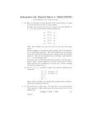
While searching “top-down”, we can “prune out”<br />
irrelevant subtrees using α-β-pruning. Idea: while<br />
searching the minmax tree, maintain two values:<br />
α- “maximizer can assure a score <strong>of</strong> at least α”;<br />
β- “minimizer can assure a score <strong>of</strong> at most β”;<br />
7<br />
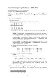
L<br />
R<br />
Player I:<br />
Player II:<br />
L<br />
R<br />
L<br />
R<br />
L R L R<br />
L R L R<br />
5 2 4 1 2 3 7<br />
1<br />
Kousha Etessami AGTA: Lecture 11
minmax search with α-β-pruning<br />
Assume, for simplicity, that players alternate moves,<br />
and root belongs to Player 1 (maximizer). Assume<br />
−1 ≤ Eval(w) ≤ +1. Score −1 (+1) means player<br />
1 definitely loses (wins). Start the search by calling:<br />
MaxVal(ǫ, −1,+1);<br />
MaxVal(w, α,β)<br />
If depth(w) ≥ MaxDepth then return Eval(w).<br />
Else<br />
for each a ∈ Act(w)<br />
α := max{α,MinVal(wa,α, β)};<br />
if α ≥ β, then return β<br />
return α<br />
MinVal(w, α,β)<br />
If depth(w) ≥ MaxDepth, then return Eval(w).<br />
Else<br />
for each a ∈ Act(w)<br />
β := min{β,MaxVal(wa,α,β)};<br />
if β ≤ α, then return α<br />
return β<br />
Heuristic game-tree search is a world <strong>of</strong> research onto<br />
itself. Please see, e.g., the references in AI texts.<br />
8<br />
Kousha Etessami AGTA: Lecture 11
9<br />
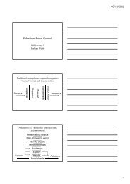
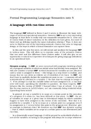
boolean circuits<br />
as finite extensive PI-games<br />
Boolean circuits can be viewed as a zero-sum PIgame,<br />
between AND and OR: OR the maximizer,<br />
AND the minimizer. (negations “pushed down” to bottom.)<br />
This is a win-lose PI-game: no chance nodes and<br />
the only possible pay<strong>of</strong>fs u(s 1 , s 2 ) are 1 and −1.<br />
0 1<br />
⇓<br />
L<br />
R<br />
Player I:<br />
Player II:<br />
L<br />
R<br />
L<br />
R<br />
L L R<br />
L L R<br />
−1 −1 1 −1 −1 1<br />
Note: game tree can be exponentially bigger, but<br />
efficient bottom-up algorithm works directly on circuit.<br />
Kousha Etessami AGTA: Lecture 11
10<br />
Ok, let’s try to generalize<br />
to infinite zero-sum games<br />
For a (possibly infinite) zero-sum 2-player PI-game,<br />
we would like to similarly define the game to be<br />
“determined” if<br />
max min u(s 1 ,s 2 ) = min max u(s 1 ,s 2 )<br />
s 1 ∈S 1 s 2 ∈S 2 s 2 ∈S 2 s 1 ∈S 1<br />
But, for infinite games max & min may not exist!<br />
Instead, let’s define an (infinite) zero-sum game to<br />
be determined (have a value) if:<br />
sup inf u(s 1 ,s 2 ) = inf sup u(s 1 ,s 2 )<br />
s 1 ∈S 1<br />
s 2 ∈S 2 s 2 ∈S 2 s 1 ∈S 1<br />
In the simple setting <strong>of</strong> infinite win-lose PI-games<br />
(2 players, zero-sum, no chance nodes, and only<br />
pay<strong>of</strong>fs are 1 and −1), this definition says a game<br />
is determined precisely when one player or the other<br />
has a winning strategy: a strategy s ∗ 1 ∈ S 1 such<br />
that for any s 2 ∈ S 2 , u(s ∗ 1, s 2 ) = 1 (and vice versa<br />
for player 2).<br />
Question: Is every win-lose PI-game determined?<br />
Answer: No .......<br />
Kousha Etessami AGTA: Lecture 11
determinacy and its boundaries<br />
For win-lose PI-games, we can define the pay<strong>of</strong>f<br />
function by providing the set Y = u −1<br />
1 (1) ⊆ Ψ T,<br />
<strong>of</strong> complete plays on which player 1 wins (player 2<br />
necessarily wins on all other plays).<br />
If, additionally, we assume that players alternate<br />
moves, we can specify such a game as G = 〈T,Y 〉.<br />
Fact Even for the binary tree T = {L,R} ∗ , there<br />
are sets Y ⊆ Ψ T , such that the win-lose PI-game<br />
G = 〈T, Y 〉 is not determined.<br />
(This fact is not very easy to show. Its pro<strong>of</strong> uses<br />
the “axiom <strong>of</strong> choice”. See, e.g., [Mycielski, Ch. 3<br />
<strong>of</strong> Handbook <strong>of</strong> GT,1992].)<br />
Fortunately, large classes <strong>of</strong> win-lose PI-games are<br />
determined. In particular:<br />
Theorem([D. A. Martin’75]) Whenever Y is a so<br />
called “Borel set”, the game 〈Σ ∗ , Y 〉 is determined.<br />
(This is a deep theorem, with deep connections to<br />
logic and set theory. The theorem holds even when<br />
the action alphabet Σ is an infinite set. )<br />
11<br />
Kousha Etessami AGTA: Lecture 11
12<br />
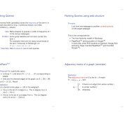
food for thought:<br />
win-lose games on finite graphs<br />
Instead <strong>of</strong> a tree, we have a finite directed graph:<br />
Start<br />
Player I:<br />
Player II:<br />
Goal<br />
• Starting at “Start”, does Player I have a strategy<br />
to “force” the play to reach the “Goal”?<br />
• Convince yourself that this is a (possibly infinite)<br />
win-lose PI-game.<br />
• Is this game determined for all finite graphs?<br />
• If so, how would you compute a winning strategy<br />
for Player 1?<br />
Kousha Etessami AGTA: Lecture 11