Computation of optical modes in axisymmetric open cavity resonators

Future Generation Computer Systems xxx (2004) xxx–xxx 

Computation of optical modes in axisymmetric open 

cavity resonators 

O. Chinellato a,∗ , P. Arbenz a , M. Streiff b , A. Witzig b 

a Institute of Computational Science, Swiss Federal Institute of Technology, CH-8092 Zurich, Switzerland 

b Integrated Systems Laboratory, Swiss Federal Institute of Technology, CH-8092 Zurich, Switzerland 

Abstract 

The computation of optical modes inside axisymmetric cavity resonators with a general spatial permittivity profile is a 

formidable computational task. In order to avoid spurious modes the vector Helmholtz equations are discretised by a mixed finite 

element approach. We formulate the method for first and second order Nédélec edge and Lagrange nodal elements. We discuss 

how to accurately compute the element matrices and solve the resulting large sparse complex symmetric eigenvalue problems. We 

validate our approach by three numerical examples that contain varying material parameters and absorbing boundary conditions 

(ABC). 

© 2004 Elsevier B.V. All rights reserved. 

Keywords: Optical mode computation; Numerical device simulation; Axisymmetric cavity; Body of revolution; Semiconductor laser; Finite 

element method; Large sparse complex symmetric eigenproblem; Jacobi–Davidson algorithm; Nédélecedge elements 

1. Introduction 

In this paper we discuss the comprehensive computation 

of optical modes inside axisymmetric cavity resonators. 

If optical gain, radiation, and absorption losses 

are taken into account, the numerical solution of complex 

symmetric eigenproblems is required. In this work 

the latter result from a finite element method (FEM) 

discretisation of the vector Helmholtz eigenproblem 

(VHEP) for open cavities. Typical resonators, the opti- 

∗ Corresponding author. 

E-mail addresses: chinellato@inf.ethz.ch (O. Chinellato), arbenz@inf.ethz.ch 

(P. Arbenz), streiff@iis.ee.ethz.ch (M. Streiff), 

witzig@iis.ee.ethz.ch (A. Witzig) 

cal modes of which are of interest, are semiconductor 

lasers [34,32], lossy waveguides [16], circular-grating 

resonators [23], photonic bandgap structures [20]. 

Until recently, new resonator designs and changes 

to the design of existing devices had to be investigated 

purely experimentally, by changing the cavity structure, 

fabricating and characterising the device. Due to 

the savings in design time and cost, comprehensive 

simulators are becoming essential tools to explore the 

design parameter space for an optimal solution. The 

foundations of such a simulator will be discussed in 

this article. 

From the point of view of computing optical modes, 

a resonator structure is described in terms of a spatially 

non-uniform complex symmetric permittivity function 

0167-739X/$ – see front matter © 2004 Elsevier B.V. All rights reserved. 

doi:10.1016/j.future.2004.09.008

2 O. Chinellato et al. / Future Generation Computer Systems xxx (2004) xxx–xxx 

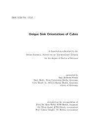
Fig. 1. Left: a possible axisymmetric cavity resonator consisting of 

different dielectric media described by a permittivity tensor ε(x). 

Right: in this example, the material arrangement can be described by 

the cross-section alone. The open resonator is composed of several 

dielectric media, ○1 ,...,○4 , surrounding air ○5 and the PML ○6 . 

ε(x), see Fig. 1. As mentioned earlier, we restrict our 

attention to axisymmetric structures. 

In order to simulate radiation leakage from the cavity 

one has to make sure that outside the cavity electromagnetic 

waves are only outgoing. If it is possible to 

extinguish the electro-magnetic waves outside the cavity 

without causing any back-scattering the computational 

domain can be truncated and made finite without 

changing the wave inside the cavity. This can be 

accomplished by an absorbing layer. 

A method that has been used for open region scattering 

problems [13], is to model the absorber as lossy 

perfectly matched layer (PML) [5,29]. The characteristics 

of the PML are first, waves propagating through 

the PML are attenuated and second, the reflection coefficient 

is zero. Such a PML is available for cylindrical 

coordinates [33] and is used here to compute the optical 

modes of open cavities. 

A simulation tool has to be capable of handling very 

general spatial permittivity profiles ε(x) to be of practical 

use. Various methods to compute optical modes 

of resonant cavities were proposed in the past, yet only 

some of them [6,22,28,30,32] are suited to treat a general 

form of a non-uniform dielectric function. 

The paper is organized as follows. In Section 2 we 

give a weak formulation of the problem. The frequency 

domain FEM formulation of the dielectric optical resonator 

problem employed in this work is related to 

[17,27,28,32]. With this approach, in principle, optical 

modes for arbitrary cavities can be computed. Typically, 

using a 2D body of revolution (BOR) expansion 

for an axisymmetric device, large sparse generalised 

complex symmetric eigenvalue problems of the 

order of approximately 500,000 have to be solved. The 

present article assesses the value of higher order finite 

element functions for this approach. In Section 3 we 

discuss a finite element discretisation of the problem 

that avoids spurious modes. We deal with the accurate 

computation of the finite element matrices and the numerical 

solution of the resulting eigenvalue problem. In 

Section 4 we present three experiments with the purpose 

to demonstrate the superiority of the quadratic 

over the linear elements and the flexibility of our approach 

in dealing with different media, including absorbing 

ones. Both these features constitute the important 

building blocks for the investigation of realistic 

optical resonators as shown in Fig. 1. We draw our 

conclusions in Section 5. 

2. Formulation of the problem 

As mentioned earlier, we want to investigate the resonance 

behaviour of axisymmetric cavities by approximatively 

solving the corresponding VHEPs. The latter 

arise (implicitly) whenever the Maxwell equations are 

used to express vector fields, which, by virtue of the 

aforementioned resonance behaviour, are assumed to 

be time-harmonic. In that case the sinusoidal ansatz is 

chosen to be F(x,t) = Re[F(x)e iωt ], where F is any of 

the considered vector fields. In this paper we only work 

with the electric field E. 

If we assume that the cavity—modelled as a 

bounded simply connected domain Ω—is nondriven 

(J = 0), charge free (ρ = 0) and possesses a 

perfectly electrically conducting (PEC) boundary Γ = 

∂Ω, Maxwell’s frequency domain equations [15] can 

be combined leading to the following problem. 

Problem 1 (VHEP). Find a vector field E ≠ 0 and 

λ ∈ C, such that 

∇×µ −1 ∇×E = λεE ∀x ∈ Ω, (1) 

∇·εE = 0 ∀x ∈ Ω, (2) 

n × E = 0 ∀x ∈ Γ (3) 

hold, where n denotes the outer surface normal on Γ = 

∂Ω and λ = ω 2 /c 2 .

O. Chinellato et al. / Future Generation Computer Systems xxx (2004) xxx–xxx 3 

Recall, that according to the constitutive relations, 

the complex symmetric tensors ε(x) and µ(x) describe 

the materials’ permittivity and permeability, respectively. 

The divergence free condition (2) serves as a filter, in 

that it discards all scalar potential field solutions, i.e. the 

fields constituting the infinite-dimensional null space 

of the curl–curl operator. Conversely, any divergence 

free solution E is guaranteed to be associated with a 

non-zero eigenvalue λ, see [11]. 

Solving these problems exactly is not possible except 

for a few particular geometries and media combinations, 

see [19]. It is therefore reasonable to compute 

approximate solutions, e.g. by applying the FEM approach. 

To this end, Problem 1 needs to be recast into 

its weak form. 

Problem 2 (weak VHEP). Find E ∈ H 0 (curl; Ω) \{0} 

and λ ∈ C, such that for all V ∈ H 0 (curl; Ω) and ψ ∈ 

H0 1(Ω) 

∫ 

∫ 

〈∇ × V, ∇×E〉 µ −1 dΩ = λ 〈V, E〉 ε dΩ, (4) 

∫ 

Ω 

Ω 

〈∇ψ, E〉 ε dΩ = 0 (5) 

hold, where 〈u, v〉 =u T v = ∑ k u kv k is a complex 

symmetric bilinear form and 〈u, v〉 A =〈u, Av〉. 

For the definition of these function spaces we refer 

to [11]. Resonator cavities, such as semiconductor 

lasers, are often axisymmetric, in which case the 

problem above is best described by means of cylinder 

coordinates 

E(x) = U(φ)Ê(r) = U(φ)[Ê r (r), Ê φ (r), Ê z (r)] T 

ψ(x) = ˆψ(r), 

Ω 

and 

where U(φ) contains the cylindrical unit vectors and 

Ê(r) represents the corresponding coordinates. The advantages 

of this transform become evident, if the material 

tensors µ and ε have no angular dependency. In 

this case a Fourier series expansion of the fields and 

potentials involved in Problem 2 

Ê(r) = 

∞∑ 

m=0 

Ê (c) 

m 

and 

(r, z) cos(mφ) + Ê(s) (r, z) sin(mφ) 

m 

ˆψ(r) = 

∞∑ 

m=0 

ˆψ (c) 

m (r, z) cos(mφ) + ˆψ m (s) (r, z) sin(mφ) 

nicely isolates all azimuthal influences. We define 

Ê m,p (c) = [Ê(c) m,r , Ê(c) m,z ]T and Ê m,p (s) = [Ê(s) m,r , Ê(s) m,z ]T , replace 

the Cartesian curl and gradient operators in 

Problem 2 with their cylindrical counterparts and finally 

apply the above Fourier expansions. The original 

problem then splits into a sequence of two-dimensional 

eigenvalue problems, one for each angular wave number 

m. Notice, that the pairwise orthogonality of the 

Fourier basis functions induces a pairwise decoupling 

of the aforementioned lower-dimensional eigenvalue 

problems. In order to keep formulations compact, let 

us introduce the bilinear forms a i (·, ·) and b j (·, ·), 

∫ 

a 1 (v, u) = r〈∇ p × v, ∇ p × u〉 ˆµ 

−1 dΩ p , 

Ω φ 

p 

∫ 

a 2 (v, u) = r −1 〈v, u〉 ˆµ −1 dΩ p, 

p 

Ω p 

∫ 

a 3 (v,u) = r −1 〈v, ∇ p (ru)〉 ˆµ −1 dΩ p, 

p 

Ω p 

∫ 

a 4 (v, u) = r −1 〈∇ p (rv), ∇ p (ru)〉 ˆµ −1 dΩ p, 

p 

Ω p 

∫ 

b 1 (v, u) = r〈v, u〉ˆεp dΩ p , 

Ω p 

∫ 

b 2 (v, u) = r〈v, u〉ˆεφ dΩ p . (6) 

Ω p 

Here, ∇ p denotes the Cartesian operator with respect 

to the coordinates (r, z). Problem 2 can now be recast 

into its cylindrical counterpart. Thereby, we neglect 

the divergence free condition, since according 

to the aforementioned filter property it suffices to 

consider only non-zero eigenvalues. For the sake of 

brevity the subscript m will be omitted in the following 

problem. 

Problem 3 (weak axisymmetric VHEP). Let m ∈ 

N 0 be a given angular wave number and Ω = 

[0, 2π] × Ω p an axisymmetric cavity. Find Ê (c) , Ê (s) ∈ 

Ĥ 0 (curl; Ω p ) \{0} and λ ∈ C, such that for all 

ˆV (c) , ˆV (s) ∈ Ĥ 0 (curl; Ω p )


a 1 ( ˆV (c) 

p , Ê(c) p ) + a 4( ˆV (s) 

φ , Ê(s) φ ) + m2 a 2 ( ˆV (c) 

p , Ê(c) p ) 

+ma 3 ( ˆV p (c) , Ê(s) φ ) + ma 3(Ê p (c) , ˆV (s) 

φ ) 

= λb 1 ( ˆV (c) 

p , Ê(c) p ) + λb 2( ˆV (s) 

a 1 ( ˆV p (s) , Ê(s) p ) + a 4( ˆV (c) 

φ 

, Ê(c) 

φ , Ê(s) φ 

φ ) + m2 a 2 ( ˆV (s) 

−ma 3 ( ˆV p (s) , Ê(c) φ ) − ma 3(Ê p (s) , ˆV (c) 

φ ) 

), (7) 

p , Ê(s) p ) 

= λb 1 ( ˆV p (s) , Ê(s) p ) + λb 2( ˆV (c) 

φ , Ê(c) φ ) (8) 

hold. 

Notice that the new function space Ĥ 0 (curl; Ω p )is 

derived from H 0 (curl; Ω) by applying the above transformations, 

leading to 

Ĥ 0 (curl; Ω p ) = 

{ 

W(r) :W ∈ ˆL 2 (Ω p ) 3 , ∇ p × W p 

∈ ˆL 2 (Ω p ), 1 r (mW p +∇ p (rW θ )) 

} 

∈ ˆL 2 (Ω p ) 2 , W p × n p = W θ = 0 ∀r ∈ Γ p , 

where Γ p = ∂Ω p \{(0, R)}, see [24]. 

In addition, we assume that the formerly mentioned 

tensors are available in diagonal form, 

i.e. ˆµ = U T µU = diag( ˆµ r , ˆµ φ , ˆµ z ) and ˆε = U T εU = 

diag(ˆε r , ˆε φ , ˆε z ). From this we derive the matrices ˆµ p = 

diag( ˆµ r , ˆµ z ) and ˆε p = diag(ˆε r , ˆε z ), in accordance with 

the definitions of the planar subcomponents Ê p 

(c) and 

Ê p (s) 

Ẇe conclude this section by pointing out that any 

solution of subproblem (7) can be transformed into 

a solution of (8) by a simple sign change in the azimuthal 

component, i.e. Ê p 

(s) = Ê(c) p and Ê(c) φ =−Ê(s) φ . 

Therefore it suffices to compute solutions of one 

subproblem—we opt for (7). 

3. Finite element discretisation 

In this section we discuss how to obtain approximate 

solutions of subproblem (7) using the FEM. We 

assume, that the cross-section Ω p has been discretised 

by means of a mixed regular mesh consisting of a set 

of triangles T and paraxial rectangles R. 

The next step in the FEM process consists in defining 

piecewise polynomial basis functions whose supports 

are spatially confined and whose span forms a 

subset of the spaces Ĥ 0 (curl; Ω p ) and Ĥ0 1(Ω p). The 

application of the weak form (7) to these finite element 

functions will then lead to a finite-dimensional approximation 

of the operator (7). 

Unfortunately the choice of appropriate finite element 

functions is very delicate, mainly because of the 

continuous operator having infinitely many zero eigenvalues. 

The degenerate null space has to be reflected by 

the discrete operator as well, in order to obtain reasonable 

approximations, see e.g. [7–9,14,21]. If this is not 

done properly, so-called spurious modes, i.e. eigenvalues 

with no physical meaning, are likely to arise. 

A possible choice that avoids this spectral pollution 

consists in modelling the field components Ê p 

(c) and 

Ê (s) 

φ 

, respectively, by Nédélec edge and modified Lagrange 

nodal element functions, as described in [25]. 

These so called hybrid element functions are guaranteed 

to reproduce a portion of the null space correctly 

and thus lead to spurious free approximations. 

It is well known, that the quality of FEM approximations 

depends on the mesh width as well as on the 

order of the element functions. In this article we will use 

both, first and second order hybrid element functions 

defined over both, triangles and paraxial rectangles. 

To be more precise, we define T 0 to be the reference 

triangle with vertices (0, 0), (1, 0) and (0, 1). 

Additionally, we introduce the simplex coordinates 

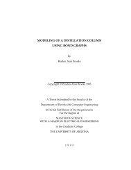
Fig. 2. Vector element functions N T i 

obtained by “cyclic rotation”. 

1 , NT i 

4 and NT i 

7 related to the bottom edge of an arbitrary triangle T i. The other vector functions can be


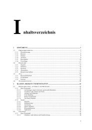
Fig. 3. DOF placement for triangles. The positions of the nodal functions are marked as white numbered dots, whereas vector functions are 

represented by means of white numbered arrows. Left: first order functions; right: second order functions including interior ones. 

ζ 1 = 1 − r − z, ζ 2 = r and ζ 3 = z. The element functions 

whose support intersect T 0 (see Fig. 2) are then 

defined as [18] 

N T 0 

i (r, z) = ζ i N T 0 

i (r, z) = ζ i ∇ p ζ i+1 − ζ i+1 ∇ p ζ i 

N T 0 

i+3 (r, z) = 4ζ i+1ζ i N T 0 

i+3 (r, z) = ζ i ∇ p ζ i+1 + ζ i+1 ∇ p ζ i 

N T 0 

i+6 (r, z) = ζ i+2(ζ i ∇ p ζ i+1 − ζ i+1 ∇ p ζ i ) 

where the indices of the ζ functions wrap in modulo 

arithmetic fashion and i = 1, 2, 3. See Fig. 3 in order 

to understand how to interpret the degrees of freedom 

(DOF). 

In analogy to T 0 , let R 0 be the reference rectangle 

with vertices (0, 0), (1, 0), (1, 1) and (0, 1). Again, 

we introduce new coordinates ζ 1 = 1 − r, ζ 2 = 1 − z, 

ζ 3 = r and ζ 4 = z. The element functions whose support 

intersect with R 0 (see Fig. 4) are then defined to 

be [18] 

N R0 

i (r, z) = ζ i ζ i+1 N R0 

(r, z) =−ζ i+1 ∇ p ζ i 

N R0 

i+4 (r, z) = 4 ζ iζ i+1 ζ i+2 N R0 

i+4 (r, z) = (1 − 2ζ i)ζ i+1 ∇ p ζ i 

N R0 

9 (r, z) = 16 ζ 1ζ 2 ζ 3 ζ 4 N R0 

i+8 (r, z) = ζ iζ i+1 ζ i+2 ∇ p ζ i+1 

where the indices of the ζ wrap in modulo arithmetic 

fashion and i = 1, 2, 3, 4. See Fig. 5 in order to understand 

how to interpret the DOF. 

i 

Note that in both cases, the left columns represent 

the nodal element functions whereas the right 

columns denote the vector element functions. Moreover, 

if the approximation is of first order, only the first 

row of functions is used in each case. For second order 

approximations, the remaining functions are incorporated 

into the discrete spaces as well. However, before 

these functions can be used, they must be (affinely) 

mapped onto each of the triangles T i and rectangles 

R j . 

The finite element functions, whose restriction to a 

single polygon has been described above, constitute the 

discrete function space, in which the desired approximations 

reside. In order to compute these approximations, 

it is necessary to construct the discrete operators 

described by the weak form (7). To this end we expand 

the field components used in Problem 3 by means of 

the finite element functions given above, i.e. 

{ } 

Ê(c) p 

ˆV p 

(c) = ∑ k 

{ } 

Ê(s) φ 

ˆV (s) = ∑ 

φ k 

{ 

xk 

˜x k 

} 

N k (r, z) 

and 

{ 

yk 

ỹ k 

} 

r −1 N k (r, z), (9) 

Fig. 4. Vector element functions N R j 

can be obtained by “cyclic rotation”. 

1 , NR j 

5 and N R j 

9 related to the bottom edge of an arbitrary paraxial rectangle R j . The other vector functions


Fig. 5. DOF placement for rectangles. The positions of the nodal functions are marked as white numbered dots, whereas vector functions are 

represented by means of white numbered arrows. Left: first order functions; right: second order functions including interior ones. 

where the element functions are now globally numbered. 

Note, that the r −1 factor in front of N k (r, z)isthe 

modification which guarantees spurious free approximations. 

Unfortunately, the price for this modification 

is a change in the set of boundary conditions prescribed 

by Ĥ 0 (curl; Ω p ). 

Inserting the finite element expansions (9) into the 

weak form (7) and considering that the latter must hold 

for all functions ˆV p (c), 

ˆV (s) 

φ , leads to an eigenvalue problem 

[ ][ ] 

A1 + m 2 A 2 mA 3 x 

Az = 

mA T 3 

A 4 y 

[ ][ ] 

B1 0 x 

= λ 

= λBz, (10) 

0 B 2 y 

where the sub–blocks A i and B j are associated with 

the corresponding bilinear forms a i (·, ·) and b j (·, ·) in 

(6). 

An important point to note is that both, the inner 

products and the tensors, are symmetric. Since the latter 

may be complex, the resulting general eigenvalue 

problem (10) turns out to be complex symmetric, as 

well. In addition, both matrices A and B will be sparse, 

due to the locally confined supports of the finite element 

functions. 

3.1. Accurate evaluation of bilinear forms 

Despite the formal simplicity of the matrix assembling 

process, care has to be taken when numerically 

evaluating the integrals given by the bilinear forms (6). 

Recall, that even though the element functions N i (r, z) 

and N j (r, z) are mere polynomials q(r, z), some of the 

integrals possess a weighting term r −1 . Explicit evaluation 

of these integrals leads to very large expressions 

which suffer from cancellation. The alternative application 

of standard numerical integration techniques, such 

as Gaussian quadrature, requires many function evaluations 

in order to obtain accurate results, which becomes 

even worse, if tensor product rules are used. Moreover, 

such straightforward numerical quadrature would lead 

to cancellation. 

To avoid these problems, we transform integrals 

over triangles into integrals over triangle boundaries, 

i.e. sums of one-dimensional integrals. By applying 

Green’s theorem we get 

∫ 

∫ 

x −1 q(x, y)dT = x −1 Q(x, y)d∂T 

T 

∂T 

= ∑ ∫ 1 

u k (x k + u k t) −1 Q(x k + u k t, y k + v k t)dt, 

k 

0 

where Q(x, y) = ∫ q(x, y)dy. The parameters u k = 

x k+1 − x k and v k = y k+1 − y k denote the differences 

between the x and y coordinates of the counterclockwise 

oriented triangle vertices (x k ,y k ) with k = 1, 2, 3. 

Integrals over paraxial rectangles are recast into 

product form and lead to integrals of the form 

∫ 

∫ 1 

x −1 q(x, y)dR = u 0 (x 0 + u 0 t) −1 

R 

[Q(x 0 + u 0 t, y 0 + v 0 ) − Q(x 0 + u 0 t, y 0 )] dt, 

0 

where again, the parameters depend on the underlying 

rectangle, i.e. (x 0 ,y 0 ) denotes its lower left corner and 

u 0 and v 0 its width and height, respectively.


Hence, the original integration problem can be reduced 

to a set of line integrals with weight function 

(α + βt) −1 , for which the construction of appropriate 

Gauss quadrature rules is feasible. Notice, that each element 

requires its own quadrature rule! Nevertheless, 

these quadrature rules can be constructed cheaply [12], 

whence the bilinear forms can be evaluated efficiently 

and accurately. 

4. Numerical experiments 

This section is devoted to the validation of the 

previously described modelling process. To this end 

we investigate cavities whose geometries and material 

arrangements admit solving (1) in closed form. The analytical 

solutions can then be compared to the approximate 

ones, obtained from solving the FEM models. 

Note that throughout this section we assume that µ = I. 

In order to compute a few of the eigenvalues of 

the generalised complex symmetric eigenvalue problem 

(10) close to a target value τ it is advisable to 

transform it into the form 

(A − σB) −1 Bz = νz, ν = (λ − σ) −1 , (11) 

where σ is a shift equal or close to the target. The latter is 

usually found by means of a related simplified problem. 

(11) is called a shift-and-invert spectral transformation 

[4] with shift σ. By means of the spectral transformation 

the eigenvalues of the matrix pencil (A; B) that are 

close to the shift become the largest in modulus of (11). 

The eigenvectors remain unchanged. 

The Arnoldi algorithm is a well-known method for 

calculating a few of the extremal eigenvalues of a large 

matrix. We use the implicitly restarted Arnoldi algorithm 

as it is implemented in the Matlab function 

eigs. eigs actually is an interface to a compiled 

routine of ARPACK [26]. The implicit restarts make 

it possible to control the memory requirements without 

losing the favourable convergence properties of the 

Arnoldi algorithm. 

The shift-and-invert spectral transformation exposes 

the interior eigenvalues close to the shift. But 

the transformation entails that a system of equations of 

the form 

(A − σB)x = By (12) 

must be solved in every step of the Arnoldi iteration. 

As our problems are not too large we use a direct solver 

to this end. Notice that it is important to permute the 

matrix A − σB to reduce fill-in, e.g. by minimum degree 

reordering. By suppressing pivoting we can save 

the symmetry of the problem, however at the expense 

of stability! When A − σB will become too large to 

be factored we will employ a variant of the Jacobi– 

Davidson algorithm, JDCS, that has been adapted to 

the complex symmetric eigenvalue problem [3]. 

4.1. A hollow cylinder cavity 

The first cavity we investigate is a hollow cylindrical 

resonator. We assume the cylinder is empty (ε = I) 

with unit radius and height (R = H = 1) and surrounded 

by a PEC layer. The exact solutions can be 

constructed by separation of variables, see [19]. Thus, 

the eigenvalues can be expressed in the form 

⎧ 

⎨ 

⎩ 

λ (TM) 

m,n,l 

λ (TE) 

m,n,l+1 

⎫ { } 

⎬ b 

2 

⎭ = m,n 

b ′ 2 

m,n 

R −2 + l 2 π 2 H −2 , 

m, l = 0, 1, 2,..., n= 1, 2, 3,... (13) 

Here b m,n denotes the nth root of the Bessel function 

J m (x) and b m,n ′ denotes the nth root of its first derivative 

J m ′ (x). Some of the roots b m,n and b m,n ′ are listed in [2]. 

This is a real eigenvalue problem. The desired eigenvalues 

are the lowest ones. In Figs. 6 and 7 the convergence 

of a few of these eigenvalues is plotted in log– 

log scale. The plots confirm the theoretically predicted 

convergence behaviour. The linear elements have linear 

convergence rate, the quadratic elements display a 

quadratic convergence rate. By consequence, the eigenvalues 

converge quadratically in case of a first order approximation 

and quartically in case of a second order 

one. 

In Table 1, another point of view of the same data is 

given. There, DpD (DOF-per-Digit) denotes the factor 

by which the number of the degrees of freedom have to 

be multiplied to gain a decimal digit in accuracy. The 

lower this factor the better. Again, it is clear that for a 

given accuracy many fewer degrees of freedom are required 

with the quadratic than with the linear elements. 

The factors for the rectangles are better than those for 

the triangles. However, the difference at least for the 

second order elements, is small.


Fig. 6. Comparison of first and second order functions over triangular elements. The plots show the relative errors of a few of the smallest 

eigenvalues w.r.t. the mesh width, using first order (thin) and second order (thick) elements. The random triangular meshes were generated 

using Matlab’s Pde tool. Left: angular wavenumber m = 0. Relative error of λ (TM) 

010 (solid), λ (TM) 

011 (dashed) and λ (TE) 

011 (dotted). Right: angular 

wavenumber m = 1. Relative error of λ (TE) 

111 (solid), λ(TM) 

110 (dashed) and λ (TM) 

111 (dotted). 

4.2. Two concentric dielectric spheres 

In this second example we consider a cavity consisting 

of two concentric dielectric spheres with radii 

a = 1 and b = 2, respectively. Moreover, the permittivity 

of the inner sphere is ε a = 10 whereas the outer 

sphere is empty (ε b = 1) and enclosed by a PEC layer. 

Notice that the use of different media can easily be 

incorporated into our model. 

The computation of the exact solution can be carried 

out following the lines of [1]. Let k = √ λ, k a = k √ ε a 

and k b = k √ ε b . Then, the characteristic equations for 

the eigenvalues can be expressed by means of the determinants 

∣ 

0 − J +(k b b) 

√ 

kb b 

− J +(k a b) 

√ 

ka b 

k a J − (k a a) 

√ 

ka a 

and 

J + (k a b) 

√ 

kb b 

− k bJ − (k b a) 

√ 

kb a 

− Y +(k b b) 

√ 

kb b 

Y + (k a b) 

√ 

kb b 

− k bJ − (k b a) 

√ 

kb a 

= 0 (14) 

∣ 

Fig. 7. Comparison of first and second order functions over rectangular elements. The plots show the relative errors of a few of the smallest 

eigenvalues w.r.t. the mesh width, using first order (thin) and second order (thick) elements. The meshes consisted of equidistant squares and 

were generated by the commercially available mesh generator of ISE. Left: angular wavenumber m = 0. Relative error of λ (TM) 

010 (solid), λ (TM) 

011 

(dashed) and λ (TE) 

011 

(dotted). Right: angular wavenumber m = 1. Relative error of λ(TE) 


110 (dashed) and λ (TM) 

111 (dotted).


Table 1 

Comparison of the DOF-per-Digit ratio between first and second order element approximations 

DpD[△] 

DpD[□] 

First order 

λ (TM) 

010 10.4 11.1 

λ (TM) 

011 10.6 10.8 

λ (TE) 

011 12.3 12.5 

λ (TE) 

111 13.3 11.1 

λ (TM) 

110 13.9 11.1 

λ (TM) 

111 14.4 11.1 

DpD[△] 

DpD[□] 

Second order 

λ (TM) 

010 3.17 3.22 

λ (TM) 

011 3.19 3.22 

λ (TE) 

011 3.47 3.20 

λ (TE) 

111 3.35 3.31 

λ (TM) 

110 3.12 3.25 

λ (TM) 

111 3.38 3.25 

l √ ε b J + (k b b) − k b bJ − (k b b) 

0 

kε 2 b √ k b b 

l √ ε a J + (k a a) − k a aJ − (k a a) 

kε 1 a √ l √ ε b J + (k b a) − k b bJ − (k b a) 

k a a 

kε 2 a √ k b a 

√ √ ka aJ 

∣ 

+ (k a a) 

kb aJ + (k b a) 

a 

a 

where J ± (·) = J l±1/2 (·) and Y ± (·) = Y l±1/2 (·) denote 

the corresponding Bessel type functions. The roots of 

Eqs. (14) and (15) correspond to the TE and TM modes, 

respectively. Note that the index l must not be smaller 

than the angular wave number m. 

The fact that the second order approximations no 

longer converge quadratically, see Fig. 8, can be ascribed 

to the geometrical discretisation of the domain. 

The two concentric semi-discs that are used to 

l √ ε b Y + (k b b) − k b bY − (k b b) 

kε 2 b √ k b b 

l √ ε b Y + (k b a) − k b bY − (k b a) 

kε 2 a √ k b a 

= 0, (15) 

√ kb aY + (k b a) 

∣ 

a 

model the cavity are approximated by regular triangular 

meshes. Consequently, their perimeter are discretised 

as polygons which reduces the approximation power of 

the quadratic elements. Strang and Fix [31] state that 

the convergence rate should be O(h 3/2 ). We observed 

an even stronger reduction of the convergence rate to 

almost linear, see Fig. 8 and Table 2. We believe that 

we can rectify this problem by introducing curvilinear 

elements. 

Fig. 8. Comparison of first and second order element functions. The plots show the relative errors w.r.t. the mesh width, using first order (thin) 

and second order (thick) elements. The meshes consisted of triangles and were generated using Matlab’s pdetool. Left: angular wavenumber 

m = 0. Relative error of λ (TM) 


011 (dashed) and λ(TE) 

011 . Right: angular wavenumber m = 1. Relative error of λ(TE) 


110 (dashed) 

and λ (TM) 

111 (dotted).


Table 2 

Comparison of the DOF-per-Digit ratio between first and second order element approximations 

DpD[△] 

First order 

λ (TM) 

010 10.1 

λ (TM) 

011 12.6 

λ (TE) 

011 12.2 

λ (TE) 

111 12.3 

λ (TM) 

110 12.4 

λ (TM) 

111 11.2 

DpD[△] 

Second order 

λ (TM) 

010 8.83 

λ (TM) 

011 8.40 

λ (TE) 

011 7.82 

λ (TE) 

111 10.3 

λ (TM) 

110 10.0 

λ (TM) 

111 9.64 

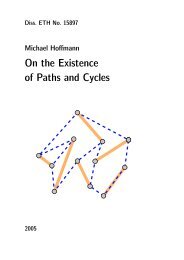
4.3. A free dielectric sphere 

To show the generality of our approach, we conclude 

this section with an open resonator cavity example. 

We consider a dielectric sphere of radius a = 1 and 

ε a = 10 immersed in free space (ε = 1) and are interested 

in its fundamental mode, i.e. the lowest TE mode 

corresponding to the angular wave number m = 1. The 

characteristic equation for this problem can be found 

in [1,10] and reads 

J l−1/2 (k √ ε a a) 

J l+1/2 (k √ ε a a) − √ 1 H (2) 

l−1/2 (k√ εa) 

εa H (2) 

l+1/2 (k√ = 0, (16) 

εa) 

where again k = √ λ and l ≥ m. The Hankel functions 

of second kind are necessary to enforce the so-called 

Sommerfeld radiation condition, i.e. a condition requiring 

that no waves are incoming from infinity. 

As explained in Section 1, the computational domain 

is truncated by means of an absorbing PML layer 

enclosed by a PEC boundary. The inner boundary of 

the 3 unit thick absorber is positioned 15 units from 

the origin and modelled according to [13]. Thus, our 

computational domain consists of different materials, 

some of which are complex. A sketch of the geometry 

is given in Fig. 9. 

Unfortunately, we were not able to solve larger 

problems with the quadratic elements because of 

the memory limitations given in Matlab. Clearly, 

the quadratic elements give a much higher accuracy 

for a given mesh than the linear ones. Due to 

the inhomogeneous grid refinement the numbers in 

Fig. 9 do not clearly reflect the theoretic expectations 

as they were observed in Experiment 1. There 

the problem was real and the grid refinement manageable. 

Fig. 9. An open cavity resonator problem with truncated simulation domain. The PML layer (light) absorbs and extinguishes outgoing waves 

and thence inhibits reflections on the outermost PEC boundary. Left: for the PML to be effective it must not be placed too close to the actual 

“cavity”. This layer is constructed such as to absorb planar waves and hence has to be put in the so-called far-field. Right: comparison of first 

and second order approximation with respect to decreasing mesh widths—the sought eigenvalue is close to 0.8805573 + 0.0965273i.


5. Conclusions 

We have given weak formulations for the axisymmetric 

vector Helmholtz problem and have discussed 

its finite element discretisation. We have shown how 

the corresponding FE matrices can be computed accurately 

and how the resulting eigenvalue problems can 

be solved. We then carried out three numerical experiments 

to show that our approach is suitable for the 

simulation of general optical resonators. 

We are still limited by our experimental environment. 

Matlab’s memory restrictions prevent us from 

dealing with the matrix sizes that are typical for real 

world problems. These large problems will also require 

factorisation-free eigenvalue solvers like the Jacobi– 

Davidson algorithm. This issues will be addressed in 

future work. 

Acknowledgements 

The work of M. Streiff and A. Witzig is supported 

by the Swiss Commission for Technology and Innovation 

(CTI) and ISE Integrated Systems Engineering 

AG, Switzerland, in the framework of the TOP NANO 

21 programme, project no. 5103.1. 

References 

[1] A. Julien, P. Guillon, Electromagnetic analysis of spherical dielectric 

shielded resonators, IEEE Trans. Microw. Theory Tech. 

34 (6) (1986) 723–729. 

[2] M. Abramowitz, I.A. Stegun, Handbook of Mathematical Functions, 

Dover, New York, NY, 1970. 

[3] P. Arbenz, M.E. Hochstenbach, A Jacobi–Davidson method 

for solving complex symmetric eigenvalue problems. Technical 

Report 374, Institute of Computational Science, ETH Zürich, 

2002 (accepted for publication in SIAM J. Sci. Comput.). 

[4] Z. Bai, J. Demmel, J. Dongarra, A. Ruhe, H. van der Vorst, 

Templates for the Solution of Algebraic Eigenvalue Problems: 

A Practical Guide, SIAM, Philadelphia, PA, 2000. 

[5] J. Berenger, A perfectly matched layer for the absorption of 

electromagnetic waves, J. Comput. Phys. 114 (2) (1995) 185– 

200. 

[6] P. Bienstman, H. Derudder, R. Baets, F. Olyslager, D. De Zutter, 

Analysis of cylindrical waveguide discontinuities using vectorial 

eigenmodes and perfectly matched layers, IEEE Trans. 

Microw. Theory Tech. 49 (2) (2001) 349–354. 

[7] D. Boffi, F. Brezzi, L. Gastaldi, On the problem of spurious 

eigenvalues in the approximation of linear elliptic problems in 

mixed form, Math. Comp. 69 (229) (1999) 121–140. 

[8] D. Boffi, P. Fernandes, L. Gastaldi, I. Perugia, Computational 

models of electromagnetic resonators: Analysis of edge element 

approximations, SIAM J. Numer. Anal. 36 (4) (1999) 1264– 

1290. 

[9] S. Caorsi, P. Fernandes, M. Raffetto, On the convergence 

of Galerkin finite element approximations of electromagnetic 

eigenproblems, SIAM J. Numer. Anal. 38 (2) (2000) 580–607. 

[10] M. Gastine, L. Courois, J.L. Dormann, Electromagnetic resonances 

of free dielectric spheres, IEEE Trans. Microw. Theory 

Tech. 15 (12) (1967) 694–700. 

[11] V. Girault, P. Raviart, Finite Element Methods for Navier– 

Stokes Equations, Springer Series in Computational Mathematics, 

vol. 5, Springer, Berlin, 1986. 

[12] G.H. Golub, J.H. Welsch, Calculation of Gauss quadrature 

rules, Math. Com. 23 (1969) 221–230. 

[13] A.D. Greenwood, J. Jin, A novel efficient algorithm for scattering 

from a complex BOR using mixed finite elements and 

cylindrical PML, IEEE Trans. Antennas and Propagation 47 (4) 

(1999) 620–629. 

[14] R. Gruber, J. Rappaz, Finite Element Methods in Linear 

Ideal Magnetohydrodynamics, Springer Series in Computational 

Physics, Springer, Berlin, 1985. 

[15] R.F. Harrington, Time-harmonic Electromagnetic Fields, 

McGraw-Hill, New York, NY, 1961. 

[16] J.M. Heaton, M.M. Bourke, S.B. Jones, B.H. Smith, K.P. Hilton, 

G.W. Smith, J.C.H. Birbeck, G. Berry, S.V. Dewar, D.R. Wight, 

Optimization of deep-etched, single-mode GaAs/AlGaAs optical 

waveguides using controlled leakage into the substrate, 

IEEE J. Lightwave Tech. 17 (2) (1999) 267–281. 

[17] S. Hyun, J. Hwang, Y. Lee, S. Kim, Computation of resonant 

modes of open resonators using the FEM and the anisotropic 

perfectly matched layer boundary condition, Microw. Opt. 

Technol. Lett. 16 (6) (1997) 352–356. 

[18] T. Itoh, G. Pelosi, P.P. Silvester (Eds.), Finite Element Software 

for Microwave Engineering, Wiley, 1996. 

[19] J.D. Jackson (Ed.), Classical Electrodynamics, 3rd edition, Wiley, 

New York, NY, 1999. 

[20] J.D. Joannopoulos, R.D. Meade, J.N. Winn, Photonic Crystals: 

Molding the Flow of Light, Princeton University Press, Princeton, 

NJ, 1995. 

[21] F. Kikuchi, Mixed and penalty formulations for finite element 

analysis of an eigenvalue problem in electromagnetism, Comput. 

Meth. Appl. Mech. Eng. 64 (1987) 509–521. 

[22] B. Klein, L.F. Register, M. Grupen, K. Hess, Numerical simulation 

of vertical cavity surface emitting lasers, OSA Opt. Express 

2 (4) (1998) 163–168. 

[23] S. Kristjansson, N. Eriksson, S.J. Sheard, A. Larsson, Circular 

grating-coupled surface-emitter with high-quality focused output 

beam, IEEE Photon. Technol. Lett. 11 (5) (1999) 497–499. 

[24] P. Lacoste, Solution of Maxwell equation in axisymmetric geometry 

by Fourier series decomposition and by use of H(rot) 

conforming finite element, Numer. Math. 84 (4) (2000) 577– 

609. 

[25] J. Lee, G.M. Wilkins, R. Mittra, Finite-element analysis of axisymmetric 

cavity resonator using a hybrid edge element technique, 

IEEE Trans. Microwave Theory Tech. 41 (11) (1993) 

1981–1987.


[26] R.B. Lehoucq, D.C. Sorensen, C. Yang, ARPACK Users’ 

Guide: Solution of Large-scale Eigenvalue Problems by Implicitly 

Restarted Arnoldi Methods, SIAM, Philadelphia, PA, 

1998. http://www.caam.rice.edu/software/ARPACK/. 

[27] N. Mahmood, B.M.A. Rahman, K.T.V. Grattan, Accurate threedimensional 

modal solutions for optical resonators with periodic 

layered structure by using the finite element method, J. 

Lightwave Technol. 16 (1) (1998) 156–161. 

[28] M.J. Noble, J.A. Lott, J.P. Loehr, Quasi-exact optical analysis 

of oxide-apertured microcavity VCSEL’s using vector finite 

elements, IEEE J. Quant. Electron. 34 (12) (1998) 2327–2339. 

[29] Z.S. Sacks, D.M. Kingsland, R. Lee, J. Lee, A perfectly matched 

anisotropic absorber for use as an absorbing boundary condition, 

IEEE Trans. Antennas Propagation 43 (12) (1996) 1460– 

1463. 

[30] J.F.P. Seurin, S.L. Chuang, Discrete Bessel transform and beam 

propagation method for modelling of vertical cavity surfaceemitting 

lasers, J. Appl. Phys. 82 (5) (1997) 2007–2016. 

[31] G. Strang, G.J. Fix, An Analysis of the Finite Element Method, 

Wellesley-Cambridge, Wellesley, MA, 1997, reprint. 

[32] M. Streiff, A. Witzig, W. Fichtner, Computing optimal modes 

for VCSEL device simulation, IEE Proc. Optoelectron. 149 (4) 

(2002) 166–173. 

[33] F.L. Teixeira, W.C. Chew, Systematic derivation of anisotropic 

PML absorbing media in cylindrical and spherical coordinates, 

IEEE Microw. Guided Wave Lett. 7 (11) (1997) 371– 

373. 

[34] A. Witzig, Modelling the optical processes in semiconductor 

lasers, Ph.D. Thesis, No. 14694, ETH, Zurich, 2002. URL 

http://e-collection.ethbib.ethz.ch/show?type=diss&nr=14694.

Computation of optical modes in axisymmetric open cavity resonators

Create successful ePaper yourself

Delete template?

Save as template?