Robust 6DOF Motion Estimation for Non-Overlapping, Multi-Camera ...

Robust 6DOF Motion Estimation for Non-Overlapping, Multi-Camera Systems
Brian Clipp 1 , Jae-Hak Kim 2 , Jan-Michael Frahm 1 , Marc Pollefeys 3 and Richard Hartley 2
1 Department of Computer Science
2 Research School of Information
3 Department of Computer Science
The University of North Carolina at Chapel Hill Sciences and Engineering ETH Zürich
Chapel Hill, NC, USA The Australian National University Zürich, Switzerland
Canberra, ACT, Australia
Abstract
This paper introduces a novel, robust approach for
6DOF motion estimation of a multi-camera system with
non-overlapping views. The proposed approach is able to
solve the pose estimation, including scale, for a two camera
system with non-overlapping views. In contrast to previous
approaches, it degrades gracefully if the motion is close to
degenerate. For degenerate motions the technique estimates
the remaining 5DOF. The proposed technique is evaluated
on real and synthetic sequences.
1. Introduction
Recently, interest has grown in motion estimation for
multi-camera systems as these systems have been used to
capture ground based and indoor data sets for reconstruction
[20, 4]. To combine high resolution and a fast framerate
with a wide field-of-view, the most effective approach
often consists of combining multiple video cameras into a
camera cluster. Some systems have all cameras mounted together
in a single location, eg. [1, 2, 3], but it can be difficult
to avoid losing part of the field of view due to occlusion (i.e.
typically requiring camera cluster placement high up on a
boom). Alternatively, for mounting on a vehicle the system
can be split into two clusters so that one can be placed on
each side of the vehicle and occlusion problems are minimized.
We will show that by using a system of two camera
clusters, consisting of one or more cameras each, separated
by a known transformation, the six degrees of freedom
(DOF) of camera system motion, including scale, can be recovered.
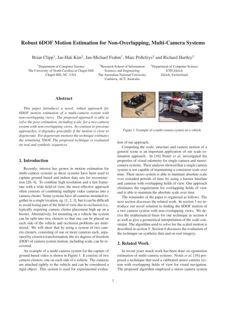
An example of a multi-camera system for the capture of
ground based video is shown in Figure 1. It consists of two
camera clusters, one on each side of a vehicle. The cameras
are attached tightly to the vehicle and can be considered a
rigid object. This system is used for experimental evalua-
Figure 1. Example of a multi-camera system on a vehicle
tion of our approach.
Computing the scale, structure and camera motion of a
general scene is an important application of our scale estimation
approach. In [16] Nistér et al. investigated the
properties of visual odometry for single-camera and stereocamera
systems. Their analysis showed that a single camera
system is not capable of maintaining a consistent scale over
time. Their stereo system is able to maintain absolute scale
over extended periods of time by using a known baseline
and cameras with overlapping fields of view. Our approach
eliminates the requirement for overlapping fields of view
and is able to maintain the absolute scale over time.
The remainder of the paper is organized as follows. The
next section discusses the related work. In section 3 we introduce
our novel solution to finding the 6DOF motion of
a two camera system with non-overlapping views. We derive
the mathematical basis for our technique in section 4
as well as give a geometrical interpretation of the scale constraint.
The algorithm used to solve for the scaled motion is
described in section 5. Section 6 discusses the evaluation of
the technique on synthetic data and on real imagery.
2. Related Work
In recent years much work has been done on egomotion
estimation of multi-camera systems. Nistér et al. [16]proposed
a technique that used a calibrated stereo camera system
with overlapping fields of view for visual navigation.
The proposed algorithm employed a stereo camera system
1

to recover 3D world points up to an unknown Euclidean
transformation. In [9] Frahm et al. introduced a 6DOF
estimation technique using a multi-camera system. Their
approach assumed overlapping camera views to obtain the
scale of the camera motion. In contrast, our technique does
not require any overlapping views. In [19] Tariq and Dellaert
proposed a 6DOF tracker for a multi-camera system
for head tracking. Their multi-camera motion estimation is
based on known 3D fiducials. The position of the multicamera
system is computed from the fiducial positions with
a MAP based optimization. Our algorithm does not require
any information about the observed scene. Therefore, it has
a much broader field of application.
Another class of approaches is based on the generalized
camera model [10, 17] of which a stereo/multi-camera system
is a special case. A generalized camera is a camera
which can have different centers of projection for each point
in the world space. An approach to the motion estimation of
a generalized camera was proposed by Stewénius et al.[18].
They showed that there are up to 64 solutions for the relative
position of two generalized cameras given 6 point correspondences.
Their method delivers a rotation, translation
and scale of a freely moving generalized camera. One of
the limitations of their approach is that centers of projection
cannot be collinear. This limitation naturally excludes all
two camera systems as well as a system of two camera clusters
where the cameras of the cluster have approximately
the same center of projection. In [12] motion estimation
for non-overlapping cameras was solved by transforming it
into the well known triangulation problem. The next section
will introduce our novel approach to estimating the 6DOF
motion of commonly used two/multi camera systems.
3. 6DOF Multi-camera Motion
The proposed approach addresses the 6DOF motion estimation
of multi-camera systems with non-overlapping
fields of view. Most previous approaches to 6DOF motion
estimation have used camera configurations with overlapping
fields of view, which allow correspondences to be
triangulated simultaneously across multiple views with a
known, rigid baseline. Our approach uses a temporal baseline
where points are only visible in one camera at a given
time. The difference in the two approaches is illustrated in
figure 2.
Our technique assumes that we can establish at least five
temporal correspondences in one of the cameras and one
temporal correspondence in any additional camera. In practice
this assumption is not a limitation, as a reliable estimation
of camera motion requires multiple correspondences
from each camera due to noise.
The essential matrix which defines the epipolar geometry
of a single freely moving calibrated camera can be estimated
from five points. Nistér proposed an efficient algo-
Figure 2. (a) Overlapping stereo camera pair, (b) Non-overlapping
multi-camera system
rithm for this estimation in [15]. It delivers up to ten valid
solutions for the epipolar geometry. The ambiguity can be
eliminated with additional points. With oriented geometry
the rotation and the translation up to scale of the camera
can be extracted from the essential matrix. Consequently a
single camera provides 5DOF of the camera motion. The
remaining degree is the scale of the translation. Given these
5DOF of multi-camera system motion (rotation and translation
direction) we can compensate for the rotation of the
system. Our approach is based on the observation that given
the temporal epipolar geometry of one of the cameras, the
position of the epipole in each of the other cameras of the
multi-camera system is restricted to a line in the image.
Hence the scale as the remaining degree of freedom of the
camera motion describes a linear subspace.
In the next section, we derive the mathematical basis of
our approach to motion recovery.
4. Two Camera System – Theory
We consider a system involving two cameras, rigidly
coupled with respect to each other. The cameras are assumed
to be calibrated. Figure 3 shows the configuration
of the two-camera system. The cameras are denoted by C 1
and C 2 , at the starting position and C ′ 1 and C ′ 2 after a rigid
motion.
We will consider the motion of the camera-pair to a new
position. Our purpose is to determine the motion using image
measurements. It is possible through standard techniques
to compute the motion of the cameras up to scale,
by determining the motion of just one of the cameras using
point correspondences from that camera. However, from
one camera, motion can be determined only up to scale. The
direction of the camera translation may be determined, but
not the magnitude of the translation. It will be demonstrated
in this paper that a single correspondence from the second
camera is sufficient to determine the scale of the motion,
that is, the magnitude of the translation. This result is summarized
in the following theorem.
Theorem 1. Let a two camera system have initial configuration
determined by camera matrices P 1 = [I | 0]
and P 2 = [R 2 | − R 2 C 2 ]. Suppose it moves rigidly to
a new position for which the first camera is specified by
P ′ 1 =[R ′ 1 | − λR ′ 1 C′ 1]. Then the scale of the translation,

λ, is determined by a single point correspondence x ′ ↔ x
seen in the second camera according to the formula
x ′⊤ Ax + λx ′⊤ Bx =0 (1)
where A = R 2 R ′ 1 [(R ′ 1 ⊤ − I)C 2 ] × R 2 ⊤ and B =
R 2 R ′ 1 [C ′ 1] × R 2 ⊤ . In this paper [a] × b denotes the skewsymmetric
matrix inducing the cross product a × b.
Figure 3. Motion of a multi-camera system consisting of two
rigidly coupled conventional cameras.
In order to simplify the derivation we assume that the coordinate
system is centered on the initial position of the first
camera, so that P 1 =[I | 0]. Any other coordinate system
is easily transformed to this one by a Euclidean change of
coordinates.
Observe also that after the motion, the first camera has
moved to a new position with camera center at λC ′ 1. The
scale is unknown at this point because in our method we
propose as a first step determining the motion of the cameras
by computing the essential matrix of the first camera
over time. This allows us to compute the motion up to scale
only. Thus the scale λ remains unknown. We now proceed
to derive Theorem 1. Our immediate goal is to determine
the camera matrix for the second camera after the motion.
First note that the camera P ′ 1 may be written as
P ′ 1 =[I | 0]
[
R
′
1 −λR ′ 1 C′ 1
0 ⊤ 1
]
= P 1 T .
where the matrix T, is the Euclidean transformation induced
by the motion of the camera pair. Since the second camera
undergoes the same Euclidean motion, we can compute the
camera P ′ 2 to be
P ′ 2 = P 2 T
[ ]
R
′
1 −λR ′ 1
= [R 2 |−R 2 C 2 ]
C′ 1
0 ⊤ 1
= [R 2 R ′ 1 |−λR 2 R ′ 1 C′ 1 − R 2 C 2 ]
= R 2 R ′ 1[I |−(λC ′ 1 + R ′ 1 ⊤ C 2 )] . (2)
From the form of the two camera matrices P 2 and P ′ 2,we
may compute the essential matrix E 2 for the second camera.
E 2 = R 2 R ′ 1[λC ′ 1 + R ′ 1 ⊤ C 2 − C 2 ] × R 2
⊤
= R 2 R ′ 1[R ′ 1 ⊤ C 2 − C 2 ] × R 2 ⊤ + λR 2 R ′ 1[C ′ 1] × R 2 ⊤ (3)
= A + λB .
Now, given a single point correspondence x ′ ↔ x as
seen in the second camera, we may determine the value of
λ, the scale of the camera translation. The essential matrix
equation x ′⊤ E 2 x =0yields x ′⊤ Ax + λx ′⊤ Bx =0, and
hence:
λ = − x′⊤ Ax
(
x ′⊤ Bx = R 2 R ′ 1[R ′
−x′⊤ 1 ⊤ C 2 − C 2 ] × R ) ⊤ 2 x
x ( ′⊤ R 2 R ′ 1 [C′ 1 ] ×R ) (4)
⊤ 2 x
.
So each correspondence in the second camera provides a
measure for the scale. In the next section we give a geometric
interpretation for this constraint.
4.1. Geometric Interpretation
The situation may be understood via a different geometric
interpretation, shown in Figure 4. We note from (2)
that the second camera moves to a new position C ′ 2(λ) =
R ′ 1 ⊤ C 2 + λC ′ 1. The locus of this point for varying values
of λ is a straight line with its direction vector C ′ 1, passing
through the point R ′ 1 ⊤ C 2 . From its new position, the camera
observes a point at position x ′ in its image plane. This
image point corresponds to a ray v ′ along which the 3D
point X must lie. If we think of the camera as moving along
the line C ′ 2(λ) (the locus of possible final positions of the
second camera center), then this ray traces out a plane Π;
the 3D point X must lie on this plane.
On the other hand, the point X is also seen (as image
point x) from the initial position of the second camera, and
hence lies along a ray v through C 2 . The point where this
ray meets the plane Π must be the position of the point X.
In turn this determines the scale factor λ.
4.2. Critical configurations
This geometric interpretation allows us to identify critical
configurations in which the scale factor λ cannot be
determined. As shown in Figure 4, the 3D point X is the
intersection of the plane Π with a ray v through the camera
center C 2 . If the plane does not pass through C 2 , then the
point X can be located as the intersection of plane and ray.
Thus, a critical configuration can only occur when the plane
Π passes through the second camera center, C 2 .
According to the construction, the line C ′ 2(λ) lies on the
plane Π. For different 3D points X, and corresponding image
measurement x ′ , the plane will vary, but always contain
the line C ′ 2(λ). Thus, the planes Π corresponding to different
points X form a pencil of planes hinged around the

Figure 6. Critical motion due to constant rotation rate
Figure 4. The 3D point X must lie on the plane traced out by the
ray corresponding to x ′ for different values of the scale λ. Italso
lies on the ray corresponding to x through the initial camera center
C 2.
(R ′ 1 ⊤ C 2 − C 2 ) × C ′ 1 = 0, or rearranging this expression,
and observing that the vector C 2 × C ′ 1 is perpendicular to
the plane of the three camera centers C 2 , C ′ 1 and C 1 (the
last of these being the coordinate origin), we may state:
Theorem 2. The critical condition for singularity for scale
determination is
(R ′ 1 ⊤ C 2 ) × C ′ 1 = C 2 × C ′ 1 .
Figure 5. Rotation Induced Translation to Translation Angle
axis line C ′ 2(λ). Unless this line actually passes through
C 2 , there will be at least one point X for which C 2 does not
lie on the plane Π, and this point can be used to determine
the point X, and hence the scale.
Finally, if the line C ′ 2(λ) passes through the point C 2 ,
then the method will fail. In this case, the ray corresponding
to any point X will lie within the plane Π, and a unique
point of intersection cannot be found.
In summary, if the line C ′ 2(λ) does not pass through the
initial camera center C 2 , almost any point correspondence
x ′ ↔ x may be used to determine the point X and the translation
scale λ. The exceptions are point correspondences
given by points X that lie in the plane defined by the camera
center C 2 and the line C ′ 2(λ) as well as far away points
for which Π and v are almost parallel.
If on the other hand, the line C ′ 2(λ) passes through the
center C 2 , then the method will always fail. It may be
seen that this occurs most importantly if there is no camera
rotation, namely R ′ 1 = I. In this case, we see that
C ′ 2(λ) =C 2 + λC ′ 1, which passes through C 2 . It is easy to
give an algebraic condition for this critical condition. Since
C ′ 1 is the direction vector of the line, the point C 2 will
lie on the line precisely when the vector R ′ 1 ⊤ C 2 − C 2 is
in the direction C ′ 1. This gives a condition for singularity
In particular, the motion is not critical unless the axis of rotation
is perpendicular to the plane determined by the three
camera centers C 2 , C ′ 1 and C 1 .
Intuitively, critical motions occur when the rotation induced
translation R ′ 1 ⊤ C 2 − C 2 is aligned with the translation
C ′ 1. In this case the angle Θ in Fig. 5 is zero. The
most common motion which causes a critical condition is
when the camera system translates but has no rotation. Another
common but less obvious critical motion occurs when
both camera paths move along concentric circles. This configuration
is illustrated in figure 6. A vehicle borne multicamera
system turning at a constant rate undergoes critical
motion, but not when it enters and exits a turn.
Detecting critical motions is important to determining
when the scale estimates are reliable. One method to determine
the criticality of a given motion is to use the approach
of [8]. We need to determine the dimension of the space
which includes our estimate of the scale. To do this we
double the scale λ and measure the difference in the fraction
of inliers to the essential matrix of our initial estimate
and the doubled scale essential matrix. If a large proportion
of inliers are not lost when the scale is doubled then
the scale is not observable from the data. If the scale is observable
the deviation from the estimated scale value would
cause the correspondences to violate the epipolar constraint,
which means they are outliers to the constraint for the doubled
scale. When the scale is ambiguous doubling the scale
does not cause correspondences to be classified as outliers.
This method proved to work practically on real data sets.

Figure 7. Algorithm for estimating 6DOF motion of a multicamera
system with non-overlapping fields of view.
5. Algorithm
Figure 7 shows an algorithm to solve relative motion
of two generalized cameras from 6 rays with two centers
where 5 rays meet one center and sixth ray meets the other
center. First, we use 5 correspondences in one ordinary
camera to estimate an essential matrix between two frames
in time. The algorithm used to estimate the essential matrix
from 5 correspondences is the method by Nistér [15]. It
is also possible to use a simpler algorithm which gives the
same result developed by Li and Hartley [13]. The 5 correspondences
are selected by the RANSAC (Random Sample
Consensus) algorithm [7]. The distance between a selected
feature and its corresponding epipolar line is used as an inlier
criterion in the RANSAC algorithm. The essential matrix
is decomposed into a skew-symmetric matrix of translation
and a rotation matrix. When decomposing the essential
matrix into rotation and translation the chirality constraint
is used to determine the correct configuration [11]. At this
point the translation is recovered up to scale.
To find the scale of translation, we use Eq. 4 with
RANSAC. One correspondence is randomly selected from
the second camera and is used to calculate a scale value
based on the constraint given in Eq. 4. We have also used
a variant of the pbM-Estimator [6] to find the initial scale
estimate with similar results and speed to the RANSAC approach.
This approach forms a continuous function based
on the discrete scale estimates from each of the correspondences
in the second camera and selects the maximum of
that continuous function as the initial scale estimate.
Based on this scale factor, the translation direction and
rotation of the first camera, and the known extrinsics between
the cameras, an essential matrix is generated for the
second camera. Inlier correspondences in the second camera
are then determined based on their distance to the epipolar
lines. A linear least squares calculation of the scale
factor is then made with all of the inlier correspondences
from the second camera. This linear solution is refined
with a non-linear minimization technique using the GNC
function [5] which takes into account the influence of all
correspondences, not just the inliers of the RANSAC sample,
in calculating the error. This error function measures
the distance of all correspondences to their epipolar lines
and smoothly varies between zero for perfect correspondence
and one for an outlier with distance to the epipolar
line greater than some threshold. One could just as easily
take single pixel steps from the initial linear solution in the
direction which maximizes inliers, or equivalently minimizing
the robust error function. The non-linear minimization
simply allows us to select step sizes depending on the sampled
Jacobian of the error function, which should converge
faster than single pixel steps and allows for sub-pixel precision.
Following refinement of the scale estimate, the inlier correspondences
of the second camera are calculated and their
number is used to score the current RANSAC solution. The
final stage in the scale estimation algorithm is a bundle adjustment
of the multi-camera system’s motion. Inliers are
calculated for both cameras and they are used in a bundle
adjustment refining the rotation and scaled translation of the
total, multi-camera system.
While this algorithm is described for a system consisting
of two cameras it is relatively simple to extend the algorithm
to use any number of rigidly mounted cameras. The
RANSAC for the initial scale estimate, initial linear solution
and non-linear refinement are performed over correspondences
from all cameras other than the camera used in
the five point pose estimate. The final bundle adjustment is
then performed over all of the system’s cameras.
6. Experiments
We begin with results using synthetic data to show the algorithm’s
performance over varying levels of noise and different
camera system motions. Following these results we
show the system operating on real data and measure its performance
using data from a GPS/INS (inertial navigation
system). The GPS/INS measurements are post processed
and are accurate to 4cm in position and 0.03 degrees in rotation,
providing a good basis for error analysis.
6.1. Synthetic Data
We use results on synthetic data to demonstrate the performance
of the 6DOF motion estimate in the presence of
varying levels of gaussian noise on the correspondences
over a variety of motions. A set of 3D points was generated
within the walls of an axis-aligned cube. Each cube wall
consisted of 5000 3D points randomly distributed within a
20m x 20m x 0.5m volume. The two-camera system, which
has an inter-camera distance of 1.9m,a100 o angle between

Figure 8. Angle Between True and Estimated Rotations, Synthetic
Results of 100 Samples Using Two Cameras
Figure 10. Scaled Translation Vector Error, Synthetic Results of
100 Samples Using Two Cameras
Figure 9. Angle Between True and Estimated Translation Vectors,
Synthetic Results of 100 Samples Using Two Cameras
Figure 11. Scale Ratio, Synthetic Results of 100 Samples Using
Two Cameras
optical axes and non-overlapping fields of view, is initially
positioned at the center of the cube, with identity rotation.
A random motion for the camera system was then generated.
The camera system’s rotation was generated from a
uniform ±6 o distribution sampled independently in each
Euler angle. Additionally, the system was translated by a
uniformly distributed distance of 0.4m to 0.6m in a random
direction. A check for degenerate motion is performed by
measuring the distance between the epipole of the second
camera (see Fig. 3) due to rotation of the camera system and
the epipole due to the combination of rotation and translation.
Only results of non-degenerate motions with epipole
separations equivalent to a 5 o angle between the translation
vector and the rotation induced translation vector(see Fig. 5)
are shown. Results are given for 100 sample motions for
each of the different values of normally distributed, zero
mean Gaussian white noise added to the projections of the
3D points into the system’s cameras. The synthetic cameras
have calibration matrices and fields of view which match
the cameras used in our real multi-camera system. Each
real camera has an approximately 40 o x 30 o field of view
and a resolution of 1024 x 768 pixels.
Results on synthetic data are shown in figures 8 to
11. One can see that the system is able to estimate the
rotation (Fig. 8) and translation direction (Fig. 9) well
given noise levels that could be expected using a 2D feature
tracker on real data. Figure 10 shows a plot of
‖T est − T true ‖ / ‖T true ‖. This ratio measures both the accuracy
of the estimated translation direction, as well as
the scale of the translation and would ideally have a value
of zero because the true and estimated translation vectors
would be the same. Given the challenges of translation estimation
and the precise rotation estimation we use this ratio
as the primary performance metric for the 6DOF motion estimation
algorithm. The translation vector ratio along with
the rotation error plot demonstrate that the novel system performs
well given a level of noise that could be expected in
real tracking results.
6.2. Real data
For a performance analysis on real data we collected
video using an eight camera system mounted on a vehicle.
The system included a highly accurate GPS/INS unit which
allows comparisons of the scaled camera system motion calculated
with our method to ground truth measurements. The
eight cameras have almost no overlap to maximize the total
field of view and are arranged in two clusters facing toward
the opposite sides of the vehicle. In each cluster the camera
centers are within 25cm of each other. A camera cluster is
shown in Fig. 1. The camera clusters are separated by approximately
1.9m and the line between the camera clusters
is approximately parallel with the rear axle of the vehicle.
Three of the four cameras in each cluster cover a horizontal
field of view on each side of the vehicle of approximately
120 o x 30 o . A fourth camera points to the side of the vehicle
and upward. Its principle axis has an angle of 30 o with
the horizontal plane of the vehicle which is colinear with
the optical axes of the other three cameras.

Figure 12. Angle Between True and Estimated Translation Vectors,
Real Data with Six Cameras
Figure 15. Scaled Translation Vector Difference from Ground
Truth, Real Data with Six Cameras
‖T est−T true‖
‖T true‖
0.23 ± 0.19
‖T est‖
‖T true‖
0.90 ± 0.28
Table 1. Relative translation vector error including angle and error
of relative translation vector length mean ± std.dev.
Figure 13. Angle Between True and Estimated Rotations, Real
Data with Six Cameras
Figure 14. Scale Ratio, Real Data with Six Cameras
In these results on real data we take advantage of the
fact that we have six horizontal cameras and use all of the
cameras to calculate the 6DOF system motion. The upward
facing cameras were not used because they only recorded
sky in the sequence. For each pair of frames recorded at
different times, each camera in turn is selected and the five
point pose estimate is performed for that camera using correspondences
found using a KLT [14] 2D feature tracker.
The other cameras are then used to calculate the scaled motion
of the camera system using the five point estimate from
the selected camera as an initial estimate of the camera system
rotation and translation direction. The 6DOF motion
solution for each camera selected for the five point estimate
is scored according to the fraction of inliers of all other cameras.
The motion with the largest fraction of inliers is selected
as the 6DOF motion for the camera system.
In table 1 we show the effect of critical motions described
in section 4.2 over a sequence of 200 frames. Crit-
ical motions were detected using the QDEGSAC [8] approach
described in that section. Even with critical motion
the system degrades to the standard 5DOF motion estimation
from a single camera and only the scale remains ambiguous
as shown by the translation direction and rotation
angle error in Figures 12 and 13. This graceful degradation
to the one camera motion estimation solution means that the
algorithm solves for all of the possible degrees of freedom
of motion given the data provided to it.
In this particular experiment the system appears to consistently
underestimate the scale with our multi-camera system
when the motion is non-critical. This is likely due to a
combination of error in the camera system extrinsics and
error in the GPS/INS ground truth measurements.
Figure 16 shows the path of the vehicle mounted multicamera
system and locations where the scale can be estimated.
From the map it is clear that the scale cannot be
estimated in straight segments as well as in smooth turns.
This is due to the constant rotation rate critical motion condition
described in section 4.2. We selected a small section
of the camera path circled in figure 16 and used a calibrated
structure from motion (SfM) system similar to the system
used in [15] to reconstruct the motion of one of the system’s
cameras. For a ground truth measure of scale error
accumulation we scaled the distance traveled by a camera
between two frames at the beginning of this reconstruction
to match the true scale of the camera motion according to
the GPS/INS measurements. Figure 17 shows how error
in the scale accumulates over the 200 frames (recorded at
30 frames per second) of the reconstruction. We then processed
the scale estimates from the 6DOF motion estimation
system with a Kalman filter to determine the scale of
the camera’s motion over many frames and measured the
error in the SfM reconstruction scale using only our algorithm’s
scale measurements. The scale drift estimates from

Figure 16. Map of vehicle motion showing points where scale can
be estimated
Figure 17. Scaled structure from motion reconstruction
the 6DOF motion estimation algorithm clearly measure the
scale drift and provide a measure of absolute scale.
7. Conclusion
We have introduced a novel algorithm that determines
the 6DOF motion of a multi-camera system with nonoverlapping
fields of view. We have provided a complete
analysis of the critical motions of the multi-camera system
that make the absolute scale unobservable. Our algorithm
can detect these critical motions and gracefully degrades to
the estimation of the epipolar geometry. We have demonstrated
the performance of our solution through both synthetic
and real motion sequences. Additionally, we embedded
our novel algorithm in a structure from motion system
to demonstrate that our technique allows the determination
absolute scale without requiring overlapping fields of view.
References
[1] Immersive Media Camera Systems Dodeca 2360,http://
www.immersivemedia.com/.
[2] Imove GeoView 3000, http://www.imoveinc.com/
geoview.php.
[3] Point Grey Research Ladybug2, http://www.ptgrey.
com/products/ladybug2/index.asp.
[4] A. Akbarzadeh, J.-M. Frahm, P. Mordohai, B. Clipp, C. Engels,
D. Gallup, P. Merrell, M. Phelps, S. Sinha, B. Talton,
L. Wang, Q. Yang, H. Stewenius, R. Yang, G. Welch,
H. Towles, D. Nister, and M. Pollefeys. Towards urban 3d
reconstruction from video. In Proceedings of 3DPVT, 2006.
[5] A.BlakeandA.Zisserman. Visual reconstruction. MIT
Press, Cambridge, MA, USA, 1987.
[6] H. Chen and P. Meer. Robust regression with projection
based m-estimators. In 9th ICCV, volume 2, pages 878–885,
2003.
[7] M. A. Fischler and R. C. Bolles. Random sample consensus:
a paradigm for model fitting with applications to image analysis
and automated cartography. Commun. ACM, 24(6):381–
395, 1981.
[8] J. Frahm and M. Pollefeys. Ransac for (quasi-)degenerate
data (qdegsac). pages I: 453–460, 2006.
[9] J.-M. Frahm, K. Köser, and R. Koch. Pose estimation for
Multi-Camera Systems. In DAGM, 2004.
[10] M. D. Grossberg and S. K. Nayar. A general imaging model
and a method for finding its parameters. In ICCV, pages
108–115, 2001.
[11] R. I. Hartley and A. Zisserman. Multiple View Geometry
in Computer Vision. Cambridge University Press, ISBN:
0521540518, second edition, 2004.
[12] J.-H. Kim, J.-M. Frahm, M. Pollefeys, and R. Hartley. Visual
odometry for non-overlapping views using second order
cone programming. In ACCV, 2007.
[13] H. Li and R. Hartley. Five-point motion estimation made
easy. In ICPR (1), pages 630–633. IEEE Computer Society,
2006.
[14] B. Lucas and T. Kanade. An Iterative Image Registration
Technique with an Application to Stereo Vision. In Int. Joint
Conf. on Artificial Intelligence, pages 674–679, 1981.
[15] D. Nistér. An efficient solution to the five-point relative
pose problem. In Int. Conf. on Computer Vision and Pattern
Recognition, pages II: 195–202, 2003.
[16] D. Nistér, O. Naroditsky, and J. Bergen. Visual odometry. In
IEEE Computer Society Conference on Computer Vision and
Pattern Recognition, volume 1, pages 652–659, 2004.
[17] R. Pless. Using many cameras as one. In CVPR03, pages II:
587–593, 2003.
[18] H. Stewénius, D. Nistér, M. Oskarsson, and K. Åström. Solutions
to minimal generalized relative pose problems. In
Workshop on Omnidirectional Vision, Beijing China, Oct.
2005.
[19] S. Tariq and F. Dellaert. A Multi-Camera 6-DOF Pose
Tracker. In IEEE and ACM International Symposium on
Mixed and Augmented Reality (ISMAR), 2004.
[20] M. Uyttendaele, A. Criminisi, S. Kang, S. Winder,
R. Szeliski, and R. Hartley. Image-based interactive exploration
of real-world environments. IEEE Computer Graphics
and Applications, 24(3):52–63, 2004.