Equation-Based Modeling of Variable-Structure Systems

Diss. ETH No. 18924
Equation-Based Modeling of
Variable-Structure Systems
A dissertation submitted to the
Swiss Federal Institute of Technology, Zürich
for the degree of
Doctor of Sciences
presented by
Dirk Zimmer
MSc. ETH in Computer Sciences
born June 16, 1981
citizen of Germany
accepted on the recommendation of
Prof. Dr. Walter Gander, examiner
Prof. Dr. François E. Cellier, co-examiner
Prof. Dr. Peter Widmayer, co-examiner
2010

The most important decision
in language design concerns
what is to be left out.
— Niklaus Wirth

Zusammenfassung
Gleichungsbasierte Sprachen haben sich zu einem verbreiteten Werkzeug für
die Modellierung und Simulation physikalischer Systeme entwickelt. Ihr deklarativer
Stil ermöglicht die Formulierung eigenständiger Modelle, ohne systemspezifische
Belange berücksichtigen zu müssen. Der Begriff strukturvariable
Systeme bezeichnet Modelle, deren Gleichungen sich zur Simulationszeit
ändern. Diese Modelklasse wird im Allgemeinen von M&S Umgebungen nicht
unterstützt. Den gegenwärtigen Sprachen mangelt es an der notwendigen
Ausdrucksstärke, und weitere Einschränkungen werden von den zugehörigen
Simulatoren erzwungen. Diese Dissertation erforscht im Allgemeinen die
Modellierung strukturvariabler Systeme innerhalb gleichungsbasierter Sprachen.
Zu diesem Forschungszweck wurde eine neue Sprache entwickelt, die sich
an die prominente Sprache Modelica anlehnt. Durch Verallgemeinerung bestehender
Sprachwerkzeuge wird nicht nur eine einfachere Sprache sondern auch
mehr Ausdrucksstärke ermöglicht. Die neue Sprache befähigt den Modellierer
folglich zur Beschreibung von nahezu beliebigen strukturellen Veränderungen.
Eine zugehörige Simulationsumgebung unterstützt diese neue Sprache und
beinhaltet neue, dynamische Methoden für die Indexreduktion differentialalgebraischer
Gleichungssysteme. Vier Modelle aus unterschiedlichen Anwendungsgebieten
zeigen beispielhaft die Verwendung der Sprache und belegen
die Vorzüge der vorgeschlagenen Methodik.

Abstract
Equation-based languages have become a prevalent tool for the modeling and
simulation (M&S) of physical systems. Their declarative style enables the design
of self-contained models that are liberated from system-specific computational
aspects. Variable-structure systems form a collective term for models,
where equations change during the time of simulation. This class of models
is generally not supported in M&S frameworks. The current languages lack
the required expressiveness, and further limitations are imposed by technical
aspects of the corresponding simulation framework. This thesis explores
the modeling of variable-structure systems for equation-based languages in
full generality. For this research purpose, a new modeling language has been
designed based on the prominent language Modelica. By generalizing prevalent
language constructs, the new language becomes not only simpler but
also more expressive. In this way, almost arbitrary structural changes in the
set of equations can be described. A corresponding simulation environment
supports the new language and incorporates new and dynamic methods for
index-reduction of differential-algebraic equation systems. Models of four systems
of different domains exemplify the use of the language and demonstrate
the robustness of the proposed modeling methodology.

Acknowledgments
First and foremost, I am deeply indebted to my advisor Prof. François E.
Cellier. He put an extraordinary amount of confidence in me and provided
me with the liberty to work on a topic of my choice. Whenever necessary, he
challenged me and made me become a more complete researcher. Always, he
was there to help and his rich body of experience offers an invaluable support
for a young researcher. In the same way, I am very grateful for the support
and guidance of Prof. Walter Gander. His constant trust and his altruistic
generosity promoted an inspiring research environment and a highly enjoyable
working atmosphere. I would also like to thank Prof. Peter Widmayer for
reviewing my thesis and being part of the examination committee.
Since also scientists are subject to mundane belongings and cannot retreat
themselves to a purely intellectual world, financial support is necessary.
This research project was generously sponsored by the Swiss National Science
Foundation (SNF Project No. 200021-117619/1). I am indebted to this organization
and I want to thank as well the Computer Science Department of
ETH for further financing.
As researcher, one becomes part of a community. In my case, this was the
Modelica community. The corresponding organization and conference provided
an ideal platform for my research results and promoted a very fruitful
interchange with research fellows. Hence, I greatly appreciate the work and
company of all these people that created, sustain and enrich this community.
In particular, these are Peter Aaronson, Bernhard Bachmann, Felix Breitenecker,
David Broman, Francesco Casella, Peter Fritzson, George Giorgidze,
Henrik Nilsson, Christoph Nytsch-Geussen, Martin Otter, Victorino Sanz,
Michael Tiller, and many, many others. Outside this community, I enjoyed
especially the discussions with Luc Bläser and Ernesto Kofman.
The ups and downs of everyday working life, I shared with my fellow PhD
students at ETH Zrich. Our research group was formed out of interesting
and open-minded people, and although, we all worked on different research
topics we spent a highly enjoyable time together. Hence, I want to express my
gratitude to Cyril Flaig, Pedro Gonnet, Hua Guo, Alain Lehmann, Martin
Müller, Christoph Vömel, Marcus Wittberger, and Marco Wolf. Furthermore,

VIII
I would like to thank Steven Armstrong, Beatrice Gander and Bettina Gronau
for all their administrative help during these four years. Many thanks go to
Prof. Peter Arbenz for his help on the research proposal.
A PhD Dissertation at ETH is not confined to research work only; it
rightfully includes the teaching work as well. I had the pleasure to be the
leading assistant of a programming course for three years. I was supported
by an extremely competent and motivated group of assistants that increased
the quality of education with their selfless effort. Also the helping assistants
(still being students themselves) proved to be very talented teachers. I want
to thank all of you.
During my PhD, I could attend to two MS Thesis of extraordinary quality
from the University of Applied Sciences Vorarlberg. I want to congratulate
Markus Andres and Thomas Schmitt once more for their fantastic work. This
was a very fruitful and highly enjoyable collaboration.
Last but certainly not least, I want to express my gratitude to my family
and all my friends. I want to thank you for your patience with me, for all
the help I received, for the sorrows we shared, and for the endless fun we had
together.

Contents
I Introduction 1
1 Motivation 3
1.1 Equation-Based Modeling . . . . . . . . . . . . . . . . . . . . . 4
1.2 Variable-Structure Systems . . . . . . . . . . . . . . . . . . . . 5
1.3 Outline . . . . . . . . . . . . . . . . . . . . . . . . . . . . . . . 7
2 Goals and Requirements 9
2.1 The Trebuchet . . . . . . . . . . . . . . . . . . . . . . . . . . . 9
2.2 Equation-Based Modeling . . . . . . . . . . . . . . . . . . . . . 10
2.2.1 Continuous Part . . . . . . . . . . . . . . . . . . . . . . 12
2.2.2 Discrete Part . . . . . . . . . . . . . . . . . . . . . . . . 13
2.2.3 Structural Changes . . . . . . . . . . . . . . . . . . . . . 14
2.3 Requirements of the Modeling Language . . . . . . . . . . . . . 16
2.4 Simulation . . . . . . . . . . . . . . . . . . . . . . . . . . . . . . 16
2.4.1 Continuous Systems Simulation . . . . . . . . . . . . . . 17
2.4.2 Discrete Event Simulation . . . . . . . . . . . . . . . . . 19
2.4.3 Handling of Structural Changes . . . . . . . . . . . . . . 19
2.5 Requirements of the Simulation Engine . . . . . . . . . . . . . 20
2.6 Conclusion . . . . . . . . . . . . . . . . . . . . . . . . . . . . . 21
II Equation-Based Modeling in Sol 23
3 History of Object-Oriented Modeling 25
3.1 Introduction . . . . . . . . . . . . . . . . . . . . . . . . . . . . . 25
3.2 Object-Oriented Approaches . . . . . . . . . . . . . . . . . . . . 25
3.2.1 D’Alembert’s Principle . . . . . . . . . . . . . . . . . . . 26
3.2.2 Kirchhoff’s Circuit Laws . . . . . . . . . . . . . . . . . . 27
3.2.3 Bond Graphs . . . . . . . . . . . . . . . . . . . . . . . . 29
3.2.4 Further Modeling Paradigms . . . . . . . . . . . . . . . 31

X
3.3 Computer Modeling Languages . . . . . . . . . . . . . . . . . . 32
3.3.1 MIMIC . . . . . . . . . . . . . . . . . . . . . . . . . . . 32
3.3.2 Dymola . . . . . . . . . . . . . . . . . . . . . . . . . . . 33
3.3.3 Omola . . . . . . . . . . . . . . . . . . . . . . . . . . . . 36
3.3.4 Heading to Modelica . . . . . . . . . . . . . . . . . . . . 36
4 The Modelica Standard 39
4.1 Introduction . . . . . . . . . . . . . . . . . . . . . . . . . . . . . 39
4.2 Language Constructs . . . . . . . . . . . . . . . . . . . . . . . . 40
4.3 Object-Oriented Concepts in Modelica . . . . . . . . . . . . . . 42
4.4 Support for Variable-Structure Systems . . . . . . . . . . . . . 45
4.4.1 Lack of Conditional Declarations . . . . . . . . . . . . . 45
4.4.2 No Dynamic Binding . . . . . . . . . . . . . . . . . . . . 45
4.4.3 Nontransparent Type System . . . . . . . . . . . . . . . 46
4.4.4 Insufficient Handling of Discrete Events . . . . . . . . . 46
4.4.5 Rising Complexity . . . . . . . . . . . . . . . . . . . . . 46
4.5 Existing Solutions for Variable-Structure Systems . . . . . . . . 47
4.5.1 MOSILAB . . . . . . . . . . . . . . . . . . . . . . . . . 47
4.5.2 HYBRSIM . . . . . . . . . . . . . . . . . . . . . . . . . 48
4.5.3 Chi (χ) . . . . . . . . . . . . . . . . . . . . . . . . . . . 48
4.5.4 Hydra . . . . . . . . . . . . . . . . . . . . . . . . . . . . 49
5 The Sol language 51
5.1 Motivation . . . . . . . . . . . . . . . . . . . . . . . . . . . . . 51
5.2 To Describe a Modeling Language . . . . . . . . . . . . . . . . 51
5.3 Design Principles . . . . . . . . . . . . . . . . . . . . . . . . . . 53
5.3.1 One Component Approach . . . . . . . . . . . . . . . . 54
5.4 Implementation Section . . . . . . . . . . . . . . . . . . . . . . 56
5.4.1 Declaration of Basic Variables . . . . . . . . . . . . . . . 56
5.4.2 Constants . . . . . . . . . . . . . . . . . . . . . . . . . . 57
5.4.3 Relations . . . . . . . . . . . . . . . . . . . . . . . . . . 57
5.4.4 Expressions . . . . . . . . . . . . . . . . . . . . . . . . . 58
5.4.5 Example . . . . . . . . . . . . . . . . . . . . . . . . . . . 59
5.5 Interface Section . . . . . . . . . . . . . . . . . . . . . . . . . . 60
5.5.1 Defining the Interface . . . . . . . . . . . . . . . . . . . 60
5.5.2 Accessing the interface . . . . . . . . . . . . . . . . . . . 62
5.5.3 Member Access via Parentheses . . . . . . . . . . . . . . 62
5.5.4 Member Access via Connections . . . . . . . . . . . . . 64
5.6 Header Section . . . . . . . . . . . . . . . . . . . . . . . . . . . 65
5.6.1 Definition of Constants . . . . . . . . . . . . . . . . . . 66
5.6.2 Definition and Use of Sub-Definitions . . . . . . . . . . 66
5.6.3 Type Designators . . . . . . . . . . . . . . . . . . . . . . 69

5.6.4 Means of Type Generation . . . . . . . . . . . . . . . . 69
5.7 Type System . . . . . . . . . . . . . . . . . . . . . . . . . . . . 70
5.8 Modeling of Variable-Structure Systems . . . . . . . . . . . . . 72
5.8.1 Computational Framework . . . . . . . . . . . . . . . . 72
5.8.2 If-Statement . . . . . . . . . . . . . . . . . . . . . . . . 74
5.8.3 When-Statement . . . . . . . . . . . . . . . . . . . . . . 76
5.8.4 Copy Transmissions . . . . . . . . . . . . . . . . . . . . 77
5.8.5 Initialization . . . . . . . . . . . . . . . . . . . . . . . . 77
5.8.6 Example . . . . . . . . . . . . . . . . . . . . . . . . . . . 78
5.9 Advanced Modeling Methods . . . . . . . . . . . . . . . . . . . 79
5.9.1 Prototype of Dynamic Binding . . . . . . . . . . . . . . 79
5.9.2 Aliases . . . . . . . . . . . . . . . . . . . . . . . . . . . . 81
6 Review of the Language Design 83
6.1 Good Design Decisions . . . . . . . . . . . . . . . . . . . . . . . 84
6.1.1 One-Component Approach . . . . . . . . . . . . . . . . 84
6.1.2 Environment-Based Solutions . . . . . . . . . . . . . . . 85
6.1.3 General Conditional Branches . . . . . . . . . . . . . . . 85
6.1.4 Redeclarations and Redefinitions . . . . . . . . . . . . . 86
6.2 Arguable Design Decisions . . . . . . . . . . . . . . . . . . . . . 87
6.2.1 Concerning the First-Class Status . . . . . . . . . . . . 87
6.3 Missing Language Elements . . . . . . . . . . . . . . . . . . . . 89
6.3.1 Default Values . . . . . . . . . . . . . . . . . . . . . . . 89
6.3.2 Convenient Access via Parentheses . . . . . . . . . . . . 89
6.3.3 Arrays . . . . . . . . . . . . . . . . . . . . . . . . . . . . 89
6.4 Final Evaluation . . . . . . . . . . . . . . . . . . . . . . . . . . 90
6.4.1 Simplicity . . . . . . . . . . . . . . . . . . . . . . . . . . 90
6.4.2 Maintainability . . . . . . . . . . . . . . . . . . . . . . . 90
6.4.3 Computability . . . . . . . . . . . . . . . . . . . . . . . 90
6.4.4 Verifiability . . . . . . . . . . . . . . . . . . . . . . . . . 91
XI
III Dynamic Processing of DAEs 93
7 Processing and Simulation Framework of Sol 95
7.1 Standard Processing Scheme . . . . . . . . . . . . . . . . . . . . 95
7.2 The Dynamic Framework of Sol . . . . . . . . . . . . . . . . . . 97
7.2.1 Parsing and Lexing . . . . . . . . . . . . . . . . . . . . . 98
7.2.2 Preprocessing . . . . . . . . . . . . . . . . . . . . . . . . 98
7.2.3 Instantiation and Flattening . . . . . . . . . . . . . . . . 98
7.2.4 Update and Evaluation . . . . . . . . . . . . . . . . . . 99
7.2.5 Time Integration and Event Handler . . . . . . . . . . . 99

XII
7.2.6 Dynamic DAE Processing . . . . . . . . . . . . . . . . . 100
7.3 Fundamental Entities . . . . . . . . . . . . . . . . . . . . . . . 100
7.3.1 Relations . . . . . . . . . . . . . . . . . . . . . . . . . . 103
7.3.2 Structural Changes . . . . . . . . . . . . . . . . . . . . . 104
7.3.3 Causality Graph . . . . . . . . . . . . . . . . . . . . . . 104
7.4 Evaluation within the Causality Graph . . . . . . . . . . . . . . 106
7.5 The Blackbox . . . . . . . . . . . . . . . . . . . . . . . . . . . . 107
8 Index-0 Systems 109
8.1 Requirements on a Dynamic Framework . . . . . . . . . . . . . 109
8.2 Forward Causalization . . . . . . . . . . . . . . . . . . . . . . . 109
8.3 Potential Causality . . . . . . . . . . . . . . . . . . . . . . . . . 110
8.4 Causality Conflicts and Residuals . . . . . . . . . . . . . . . . . 111
8.5 Avoiding Cyclic Subgraphs . . . . . . . . . . . . . . . . . . . . 113
8.6 States of Relations . . . . . . . . . . . . . . . . . . . . . . . . . 114
8.7 Correctness and Efficiency . . . . . . . . . . . . . . . . . . . . . 116
9 Index-1 Systems 119
9.1 Algebraic Loops . . . . . . . . . . . . . . . . . . . . . . . . . . . 119
9.1.1 Example Tearing . . . . . . . . . . . . . . . . . . . . . . 122
9.1.2 Representation in the Causality Graph . . . . . . . . . 122
9.2 Selection of Tearing Variables . . . . . . . . . . . . . . . . . . . 124
9.3 Matching Residuals . . . . . . . . . . . . . . . . . . . . . . . . . 125
9.4 Closing Algebraic Loops . . . . . . . . . . . . . . . . . . . . . . 129
9.5 Opening Algebraic Loops . . . . . . . . . . . . . . . . . . . . . 131
9.6 Fake Residuals . . . . . . . . . . . . . . . . . . . . . . . . . . . 131
9.7 Integration of the Tearing Algorithms . . . . . . . . . . . . . . 133
9.8 Correctness and Efficiency . . . . . . . . . . . . . . . . . . . . . 134
9.9 Detecting Singularites . . . . . . . . . . . . . . . . . . . . . . . 136
9.9.1 Detecting Over- and Underdetermination . . . . . . . . 136
9.9.2 Detecting False Causalizations . . . . . . . . . . . . . . 136
10 Higher-Index Systems 139
10.1 Differential-Index Reduction . . . . . . . . . . . . . . . . . . . . 139
10.2 Index Reduction by Pantelides . . . . . . . . . . . . . . . . . . 141
10.3 Tracking Symbolic Differentiation . . . . . . . . . . . . . . . . . 141
10.4 Selection of States . . . . . . . . . . . . . . . . . . . . . . . . . 143
10.4.1 Example . . . . . . . . . . . . . . . . . . . . . . . . . . . 145
10.4.2 Manual State Selection . . . . . . . . . . . . . . . . . . 146
10.5 Removing State Variables . . . . . . . . . . . . . . . . . . . . . 146
10.5.1 Example . . . . . . . . . . . . . . . . . . . . . . . . . . . 147
10.6 Correctness and Efficiency . . . . . . . . . . . . . . . . . . . . . 147

XIII
10.7 Conclusion . . . . . . . . . . . . . . . . . . . . . . . . . . . . . 148
IV Validation and Conclusions 151
11 Example Applications 153
11.1 Introduction . . . . . . . . . . . . . . . . . . . . . . . . . . . . . 153
11.2 Solsim: The Simulator Program . . . . . . . . . . . . . . . . . . 153
11.3 Electrics: Rectifier Circuit . . . . . . . . . . . . . . . . . . . . . 154
11.4 Mechanics: The Trebuchet . . . . . . . . . . . . . . . . . . . . . 157
11.4.1 The Limited Revolute Joint . . . . . . . . . . . . . . . . 160
11.4.2 Mode Changes . . . . . . . . . . . . . . . . . . . . . . . 164
11.4.3 Simulation Hints . . . . . . . . . . . . . . . . . . . . . . 165
11.4.4 Visualization . . . . . . . . . . . . . . . . . . . . . . . . 165
11.5 Population Dynamics with Genetic Adaption . . . . . . . . . . 166
11.6 Agent-Systems: Traffic Simulation . . . . . . . . . . . . . . . . 173
11.7 Summary . . . . . . . . . . . . . . . . . . . . . . . . . . . . . . 178
12 Conclusions 179
12.1 Recapitulation . . . . . . . . . . . . . . . . . . . . . . . . . . . 179
12.2 Future Work . . . . . . . . . . . . . . . . . . . . . . . . . . . . 180
12.2.1 Redundancy . . . . . . . . . . . . . . . . . . . . . . . . . 181
12.2.2 Using Data Structures . . . . . . . . . . . . . . . . . . . 182
12.3 Major Contributions . . . . . . . . . . . . . . . . . . . . . . . . 183
A Grammar of Sol 185
B Solsim Commands 187
B.1 Main Program . . . . . . . . . . . . . . . . . . . . . . . . . . . 187
B.2 Sub-Commands . . . . . . . . . . . . . . . . . . . . . . . . . . . 187
C Electric Modeling Package 189
D Mechanic Modeling Package 191

Part I
Introduction

Chapter 1
Motivation
Mankind strives to explore and predict its environment. The power of prediction
enables to establish control and dominance, and hence we pursue this
target by all means available. Computer simulation is one of these means and,
although being relatively new, it has become already an omnipresent tool in
modern science.
In order to predict the environment, we need its viable assessment first.
Many processes in our brain are devoted to this purpose, most of them acting
completely subconsciously. The conscious attempt of assessing the environment
is often denoted as modeling, especially when it is done more formally,
using a mathematical terminology. Formal modeling is at the heart of modern
science.
Modeling and simulation (M&S) are typically linked by a formal language.
Not only humans but also computers rely on formal language as communication
device. Since our ability of conscious thought bases essentially upon
our ability to speak, the language that we use will have a profound impact on
the resulting models. Modern languages that suit modeling and simulation
are not languages that have naturally developed. In contrast, they have been
specially designed to serve two purposes: One, the language shall provide a
powerful and yet convenient framework for the human modeler. Two, the
language shall be interpretable by a computer in order to perform simulation
runs or other numerical or symbolical analysis. Evidently, these two targets
do not naturally coincide, and thus their unification is the major concern of
a language designer.
This thesis presents its own language for modeling and simulation. It is
called Sol and it represents an experimental language, primarily perceived for
research purposes. Like most languages, its design builds upon a predecessor,
namely Modelica. Typical for a new language, it attempts to extend the
current boundaries of its domain. Sol aims to enable the equation-based modeling
of systems that have a variable structure. As introduction, we therefore

4 Chapter 1
examine the state of modeling based on differential-algebraic equations and
its current support of variable-structure systems.
1.1 Equation-Based Modeling
In equation-based modeling, the modeler describes the system in terms of
differential-algebraic equations. The complete model or its individual components
are thereby represented by a set of equations and its corresponding
variables. The corresponding computer language forms a general modeling
language that can be applied to various application domains.
In M&S, such languages have become increasingly more accepted and
widespread. In contrast to manually coded simulation programs (e.g. based
on MATLAB [64], C++ [89]), these languages and their corresponding environments
typically offer a number of advantages:
• A well specified modeling language drastically eases the actual modeling
process. The modeler can focus his or her energy on the actual model
creation, and does not need to worry about the underlying simulation
engine.
• The modeling language does not only enable a simulation of a given system.
It also supports the organization of knowledge. Complex systems
can be decomposed into simple, easily readable and understandable submodels.
This knowledge can be shared, promoted, and reused.
• Within a modeling language, certain components can be checked for
consistency. This allows many modeling errors to be discovered early.
The modeling process is far less error prone, and the model validation
becomes a feasible task.
• A general modeling language based upon abstract concepts of mathematics
and computer science supports the creation of sub-models from
different domains that can be coded by domain-area specialists. These
sub-models can interact with each other, thereby enabling the creating
of multi-domain models.
• Within a truly open modeling language and environment, models that
have been created once, can be reused for a longer time period, because
the model is not strictly bound to a certain programming environment.
For these reasons, a variety of equation-based modeling languages have been
developed since the 1960s. Many of these languages, however, remained within
the boundaries of academia or were not able to prevail outside their original
application domain.

Motivation 5
Fortunately, the interest in a solid standard for a general modeling language
has increased and led to the foundation of the Modelica Association [63] in
1997. It is a non-profit organization with the primary purpose of supporting
the development of a generally accepted physical systems modeling language
that forms a standard within industry and science. The association therefore
provides a general modeling language that shares its name with the organization,
and hence is also called Modelica. It is an open language, freely available
to everyone who is interested.
The Modelica language is a general modeling language, primarily intended
for modeling physical systems. At its time of introduction, it inherited several
ideas and concepts from various other modeling languages that have formerly
been of relevance, including Dymola [29] and Omola [4]. The language is
essentially based on differential-algebraic equation (DAE) systems. Modelica
offers a declarative and equation-based approach to modeling that enables the
convenient formulation of models of many different kinds of continuous processes.
In addition, Modelica offers means for event-driven discrete processes
that adequately enable the modeling of hybrid systems.
The object-oriented modeling technique embraced by Modelica enables
the modeler to cope with the increasing amount of complexity that characterizes
contemporary models for industrial applications. The knowledge can be
effectively organized, reused, and disseminated. Complexity can be portioned
out on different modeling layers and can be hidden from the end user.
Major applications are found in the mechanical, electrical, and thermodynamical
domains. Also control systems form a significant application class.
The Modelica Standard Library [37] provides model packages for all these
different domains, and hence makes the corresponding knowledge practically
available for all users. The Modelica language has successfully been applied to
a number of industrial problems, e.g. from the automotive industry [5, 26, 84],
power plants [30, 83, 85], and thermal building simulations [22, 95, 97].
1.2 Variable-Structure Systems
Whereas Modelica has become a predominant tool for many simulation tasks,
it shares a deficiency with almost all other equation-based languages: the
modeling is restricted to systems with a static structure. Yet many contemporary
models contain structural changes at simulation run-time. These systems
are typically denoted by the collective term: variable-structure systems.
The motivations that lead to the generation of such systems are manifold:
• The structural change is caused by ideal switching processes. Classic
examples are ideal diodes in electric circuits, rigid mechanical elements

6 Chapter 1
that can break apart (e.g. a breaking pendulum), or the reconfiguration
of robot models.
• The model features a variable number of variables: This issue typically
concerns social or traffic simulations that feature a variable number of
agents or entities, respectively.
• The variability in structure is to be used for reasons of efficiency: A bent
beam should be modeled in more detail at the point of the buckling and
more sparsely in the remaining regions.
• The variability in structure results from user interaction: When the
user is allowed to create or connect certain components at run-time,
this usually reflects a structural change.
The term variable-structure system turns out to be a rather general term
that applies to a number of different modeling paradigms, such as adaptive
meshes in finite elements, discrete communication models of flexible computer
networks, etc. Within the paradigm of equation-based modeling, a structural
change is typically reflected by a change in the set of variables, and by a
change in the set of equations between these time-dependent variables. These
changes may lead to severe changes in the model structure. This concerns the
causalization of the equation system, as well as the perturbation index of the
DAE system.
There is currently hardly any language or framework that supports structural
changes to a sufficient degree. Modelica itself can only be applied in
a very restricted way. Thus, a general modeling language supporting variable
structure systems offers a number of important benefits. Such a potential
language incorporates a general modeling methodology that enables the
convenient capture of knowledge concerning variable-structure systems, and
provides means for organizing and sharing that knowledge both by industry
and science. A corresponding simulator is a valuable tool for engineering and
science education.
In concrete terms, our research is intended to aid the further extension
of current equation-based modeling frameworks, especially Modelica. This
benefits primarily the prevalent application areas of multi-body mechanics
and electronics [33].
• Ideal switching processes in electronic circuits (resulting from ideal diodes,
switches, and thyristors) can be more generally modeled. Occurring
structural singularities can be handled at run-time.
• The modeling of ideal transitions in mechanical models, like breaking
processes or the transition from friction to stiction, become a more
amenable task.

Motivation 7
Additional applications may occur in domains that are currently foreign to
Modelica. This might concern for instance:
• Hybrid economic or social simulations that contain a variable number
of entities or agents, respectively.
• Traffic simulations.
Finally, more elaborate modeling techniques become available. For instance,
multi-level models can be developed, whereby the appropriate level of detail is
chosen at simulation run-time in response to computational demands and/or
level of interest.
1.3 Outline
Unfortunately, the modeling of variable-structure systems within current equation-based
M&S frameworks is very limited. This lack of support originates
from two major problem areas:
One, there is a number of severe technical restrictions that mostly originate
from the static treatment of the DAEs. Given the current computational
framework, variability in structure cannot be properly managed, and this
prevents any potential simulation of the system.
Two, there is a lack of expressiveness in the languages. For instance,
Modelica does not provide the means that are necessary to properly formulate
structural changes. Only very simple cases can be stated.
This thesis devotes a separate part for each of these problem areas. First,
the lack of expressiveness is concerned in Part II. To this end, the history
of equation-based, object-oriented modeling languages is reviewed and the
most important concepts of the Modelica language are presented. The corresponding
enhancement toward variable-structure systems is performed by the
definition of the new language: Sol. A corresponding review of the language
design concludes this part.
Part III deals with the technical means that are required for the processing
of the Sol language. It presents a dynamic framework for the processing of
differential-algebraic equations. The new methods that are provided by this
dynamic framework aim to enable the handling of almost any arbitrary change
in the set of equations.
A broad set of examples from multiple domains is provided in Part IV.
These illustrate the modeling paradigm that is promoted by the Sol language
and serve as validation for the proposed processing methods. Finally, we
conclude this thesis by enlisting future prospects and reviewing the most
important achievements of the Sol project.

8 Chapter 1
Before we continue with the history of equation-based modeling in general,
let us look at one specific example of a variable-structure system. This shall
help us to see the requirements and difficulties that inevitably need to be
concerned for all parts of this thesis.

Chapter 2
Goals and Requirements
2.1 The Trebuchet
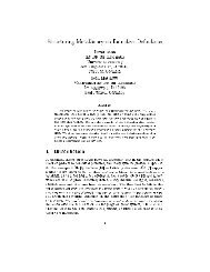
Figure 2.1: Functionality of a trebuchet.
The following example of a variable-structure system represents a seemingly
simple mechanical system: the trebuchet. Although the corresponding model
contains only a few hundred variables, it is quite complex in its internal structure.
This makes this example suitable for a quick introduction to equation-

10 Chapter 2
based object-oriented modeling. In addition, we get a first glance at the
problems that are involved with variable-structure systems.
The trebuchet is an old catapult weapon developed in the Middle Ages.
It is known for its long range and its high precision. Figure 2.1 depicts a
trebuchet and presents its functionality. Technically, it is a double pendulum
propelling a projectile in a sling. The rope of the sling is released on a
predetermined angle γ when the projectile is about to overtake the lever arm.
Furthermore, the following assumptions hold true for the modeling:
• All mechanics are planar. The positional states of any object are therefore
restricted to x, y, and the orientation angle ϕ.
• All elements are rigid.
• The rope of the sling is ideal and weightless. It exhibits an inelastic
impulse when being stretched to maximum length.
• The revolute joint of the counterweight is limited to a certain angle β (in
order to prevent too heavy back-swinging after the projectile’s release).
It also exhibits an inelastic impulse when reaching its limit.
Whereas these idealizations simplify the parameterization of the model to a
great extent, they pose serious difficulties for a general simulation environment.
Such models, although being fairly simple, can neither be modeled nor
simulated with Modelica yet — at least not in a truly object-oriented manner.
In the following section, we will sketch a proper object-oriented modeling
of the system. In doing so, we will discuss the special difficulties that occur
with respect to structural changes. This will reveal the requirements that are
put up to the modeling language and to the simulation environment. These
requirements represent valuable foresight that aids the proper design of a
suitable language.
The trebuchet example serves essentially tutorial purposes, and hence only
selected fragments will be discussed at this place. This enables the reader to
gain quickly insight to the most important problems. In addition, also more
extensive introductions to equation-based modeling in general are contained
in [37, 92] and [23]. Furthermore, the complete model of the trebuchet is
finally reviewed in Part IV of this thesis.
2.2 Equation-Based Modeling
Since the mechanical system includes the modeling of mechanic impulses, it is
a hybrid system: having both, continuously changing and discretely changing

Goals and Requirements 11
variables. Also the variability in structure represents a discrete change, not
only of the variable values but also of the set of model equations.
The most direct approach is to model the system as a whole. In modern
object-oriented modeling environments such an approach is still possible but
certainly unfavored. The resulting model would be highly complex and none
of its parts could be properly reused. For another mechanical system, the
modeling has to be redone from scratch again.
Hence the system shall be composed from sub-models that are provided
by a planar mechanical library and interact with each other by a common
interface. For this example, the following components are sufficient:
• 1 fixation component (F).
• 4 fixed translations (T0, T1, T2, T3).
• 1 revolute joint (R1).
• 1 limited revolute joint (R2).
• 2 bodies with mass and inertia (B1, B2).
• 1 ideal rope with a body attached to it (TB).
The assembly of the system from these components is represented by the
model diagram of Figure 2.2. Here the components are depicted by icons and
their connection is symbolized by solid lines. The endpoints of these lines
connect to the common interface of the components.
Figure 2.2: Model diagram of the trebuchet.

12 Chapter 2
2.2.1 Continuous Part
The component interfaces represent the contact points of the object. They
contain among other terms two sets of continuous-time variables. The first
set constitutes the potential variables that represent the position: x, y, and
the angle ϕ. The second set contains the flow variables for force and torque
f x , f y , and t.
Each component will now relate the variables of its interfaces. For instance,
the revolute joint rigidly connects the position of its two interfaces
but the angle is free. In correspondence, the torque on the joint must be zero
but it transmits arbitrary forces. This can be expressed by the following set
of algebraic equations:
ϕ 2 = ϕ 1 + ϕ
x 2 = x 1
y 2 = y 1
f x,1 + f x,2 = 0
f y,1 + f y,2 = 0
t 1 + t 2 = 0
t 2 = 0
Here, variables that belong to one of the interfaces are characterized by the
suffixes 1 and 2. Not only the angle of the revolute is of interest, but also its
velocity ω and acceleration α can be helpful variables for the simulation of the
mechanical systems. Hence the set of equations is extended by the following
two differential equations:
ω = ˙ϕ
α = ˙ω
The set of equations contains now 15 variables (12 interface variables and 3
additional internal variables) but only 9 equations and is therefore incomplete.
There are 6 equations missing. However, when the total model with all of
its components will be compiled, all equations from all components will be
collected in one set. Furthermore, equations that represent the connections
between the interfaces will be generated. These will also provide the missing
6 equations. The final system for the continuous system then contains a
mixture of pure algebraic equations and differential equations. Thus, it is
called a differential-algebraic equation (DAE) system.

Goals and Requirements 13
2.2.2 Discrete Part
The modeling of the discrete part is done in strong accordance to the continuous
part. Consequently, the interface contains also six discrete variables in
two sets. The first set contains the mean velocities during the impulse: ¯v x ,
¯v y , ¯ω. The second set consists in the corresponding force impulse and angular
momentum: P x , P y , M.
The discrete part of the model equation describes the impulse behavior.
For the revolute joint, the correspondent equation resemble its continuous
counterpart:
¯ω 2 = ¯ω 1 + ¯ω
¯v x,2 = ¯v x,1
¯v y,2 = ¯v y,1
P x,1 + P x,2 = 0
P y,1 + P y,2 = 0
M 1 + M 2 = 0
M 2 = 0
A force impulse causes a discrete change in velocity. ¯ω represents the mean
angular velocity during that impulse. This is (ω a + ω e )/2 where ω a represents
the velocity right before the impulse and ω e the velocity right after. When
an impulse is triggered, the velocity is not a continuous variable anymore but
discretely defined. The acceleration is undefined (infinite). Consequently, a
change occurs in the set of equations and a continuous equation is removed
while another is replaced by a discrete one.
z = ˙ω −→ {}
ω = ˙ϕ −→ ω = 2 ∗ ¯ω − ω a
After the force impulse, the continuous equations get immediately re-established.
Hence there are two consecutive events that are triggered within the
same frame of simulation time. We recognize that the modeling of the force
impulse can be achieved by describing a structural change. A continuous
equation is replaced by one with discrete variables. This structural change
represents only an intermediate step since the continuous equations get immediately
reestablished. Hence most modeling environments do not describe
force impulses by structural changes and use other means instead. Let us
therefore take a look at a persistent structural change that will affect the
model structure more than just temporarily.

14 Chapter 2
2.2.3 Structural Changes
The model of the trebuchet contains a second revolute joint whose angle is
limited to a certain threshold value. An elbow is one possible representation
of such a limited revolute joint. The corresponding model has two major
modes: free or fixated. The mode free is equivalent to a normal revolute joint
whereas the model equals a fixed orientation in the fixated mode. The transition
between these modes is triggered when the angle of the revolute exceeds
a predetermined limit β. Since this transition causes a discrete change in
velocity, it involves an inelastic impulse on the rigidly connected components.
Furthermore impulses from other components (as for instance the ideal rope)
need to be handled as well in this component. The different modes and their
transitions are presented in the graph of Figure 2.3, where the continuoustime
modes are depicted as round boxes and the rectangular boxes denote
discrete intermediate modes.
Figure 2.3: Mode-transition graph of the limited revolute.
Evidently, the modeling of variable-structure systems cannot restrict itself to
pure equation-based modeling. The modeling of different modes and their
transition needs to be considered as well. Furthermore events need to be
described that trigger the transition. The transition from the mode free to
fixated is triggered when the angle −ϕ exceeds the limit β. The reverse
transition is triggered when the torque t 1 on the revolute is becoming negative.
The difference between the two continuous modes is presented in Table
2.1. The variables ϕ, ω, α cease to exist in the fixated mode, and therefore,
there are 3 equations less in the corresponding set of equations. Five of the
remaining six equations are shared by both modes, and thus, the structural
change concerns only a subset of the total modeling equations.
The trebuchet contains another sub-model that exhibits force impulses
and structural changes. This component represents the torn body. Figure 2.4
depicts its three modes:

Goals and Requirements 15
1. The body is at rest as long as the rope has not been stretched.
2. The body represents a pendulum as long as the release angle β has not
been reached.
3. The body is free.
For each of these modes, different variables are used to describe the positional
state of the body. In the first mode, the position is constant and the model
contains no state variables. In the second mode, the angle and angular velocity
define the positional states, whereas the body is free in the last mode and
consequently defines the maximum of six state variables.
Free
Fixated
ϕ 2 = ϕ 1 + ϕ ϕ 2 = ϕ 1 + β
x 2 = x 1 x 2 = x 1
y 2 = y 1 y 2 = y 1
f x,1 + f x,2 = 0 f x,1 + f x,2 = 0
f y,1 + f y,2 = 0 f y,1 + f y,2 = 0
t 1 + t 2 = 0 t 1 + t 2 = 0
t 2 = 0
ω = ˙ϕ
α = ˙ω
Table 2.1: Transition form free to fixated mode.
Figure 2.4: Mode-transition graph of the torn body component.

16 Chapter 2
2.3 Requirements of the Modeling Language
So far, only a fraction of the modeling was briefly outlined. Nevertheless,
it has become evident that the modeling of variable-structure systems is a
multi-faceted task. The modeler needs to be concerned with the equationbased
modeling of continuous and discrete systems. He needs to describe
different modes and the transition between these modes. Furthermore, events
need to be formulated that trigger these transitions, and several consecutive
events must be handled within the same frame of simulation time. A modeling
language that shall suit the demands for the modeling of variable-structure
systems has therefore to fulfill a set of requirements:
• enabling the declaration of simple variables, sub-models, and their parameters;
• enabling the statement of algebraic and differential equations;
• enabling the statement of discrete assignments;
• enabling the statement of events;
• enabling the decomposition of models into sub-models by suitable object-oriented
means.
• enabling the automatic, convenient connection of those sub-models; and
• most importantly: providing a conditional statement that allows to state
all of the above in conditional form.
These are the sheer technically requirements that are put up by the modeler.
More requirements originate from organizational aspects and include further
means of object orientation. Those will be introduced within the language
definition of Chapter 5.
2.4 Simulation
Figure 2.5 displays the trajectory of the projectile as it results from the model
equations. The discrete change in velocity appears as discontinuity in the first
derivative of the plotted curve. Since a structural change always represents
a discrete event, the simulation of variable-structure systems is inherently
hybrid: containing both a continuous and a discrete part.

Goals and Requirements 17
Figure 2.5: Trajectory of the projectile.
2.4.1 Continuous Systems Simulation
In order to perform a continuous-system simulation based on DAEs, it is
desirable to transform the system of equations into a form that suits numerical
ODE (ordinary differential equations) solvers. In general, a DAE represents
a continuous system in the following form:
0 = F (ẋ p (t), x p (t), u(t), t)
where x p is the vector of potential states and u is the input vector, both
dependent on time t. It is possible to solve this system directly by corresponding
DAE solvers [48], but this is mostly inefficient since we need to
solve the initial-value problem for every integration step [12]. Hence we prefer
to achieve a transformation of F into the following state-space form f, that
is convenient for the purpose of numerical ODE solution. Here x represents
the state vector, mostly a sub-vector of x p :
ẋ(t) = f(x(t), u(t), t)
Dependent on the system F , this transformation can be non-trivial. The level
of difficulty that is encountered in this transformation is commonly described
by the perturbation index [17, 18] of the DAE system. Based on this index
definition, there are three major cases:
• Index-0 systems: For these systems, it is sufficient to order the equations
of the differential algebraic systems. The system can be solved by
forward substitution. The state vector x is equivalent to x p .
• Index-1 systems with algebraic loops: The equivalence x = x p is still
valid, but the system cannot be solved by forward substitution anymore.
In order to compute the set of algebraic variables, it is required to solve
one or several systems of equations.

18 Chapter 2
• Index-2 systems and higher index systems: Again, forward substitution
is insufficient, but the state variables of x p are also constrained by algebraic
equations in these systems. To attain an ODE form, it is required
to differentiate a subset of equations at least once. The state vector x
may now differ from the potential states in x p .
This transformation from the implicit form F to an explicit counterpart f
is consequently denoted as index reduction and represents the heart of any
compiler for equation-based modeling languages. It includes a number of
sub-tasks that can be solved by various algorithms. In Part III, the most
important of them will be discussed.
For now, let us focus on the trebuchet model. It represents an index-3
system. A subset of equations needs to be differentiated twice, and there
remain linear systems of equations to be solved. The need for differentiation
follows directly out of the object-oriented composition of the system and its
interface variables.
Differentiation
Let us suppose that the angle ϕ and the angular velocity ω of the unlimited
revolute joint are state variables that are used for time integration. Thus, we
need to determine the time derivative of the angular velocity: the angular acceleration
α. Given the current state and velocity of the system, α determines
the forces and momentums acting on the rigidly connected body components
and must be chosen in such a way that the torque on the revolute joint is
zero.
To this end, we need to compute how the angular acceleration α will
transform into the acceleration for the corresponding body components. But
only the positional variables of the components are related with each other by
the interfaces. The interface does not relate the accelerations directly. Thus,
we need to differentiate these positional variables with respect to the time.
For the trebuchet, this means that a large fraction of its variables and
thereby also of its model equations need to be symbolically differentiated.
This differentiation is even performed twice, as it is typical for mechanical
systems.
Algebraic Loops
Given the values of all state variables and external input variables, the system
cannot be completely computed by the means of forward substitution
only. Since several mass elements are rigidly connected, the forces and the
corresponding accelerations form a linear system of equations. This needs to
be solved separately. Such sub-systems are commonly denoted as algebraic

Goals and Requirements 19
loops. A DAE translator needs to extract such loops and generate code for a
numerical solution.
2.4.2 Discrete Event Simulation
The trebuchet model contains various discrete events that are triggered based
on threshold values for continuous-time variables or by preceding events.
For instance, when the limited revolute joint is about to exceed the predefined
threshold value, an event is triggered. This event causes a force impulse
that acts on multiple components and therefore must be synchronously handled
by these components. In addition, the force impulse by itself triggers
further events that are supposed to be handled consecutively but within the
same time frame.
An event handler for such systems must therefore be able to trigger events
based on continuous-time variables. Events that are triggered by the same
source shall be executed synchronously, but events must also be able to trigger
further events consecutively within the same frame of simulation time. This
requires a suitable formalism for the event handling and its comprehensible
representation in the modeling language.
2.4.3 Handling of Structural Changes
Three of the ten components in the trebuchet model exhibit structural changes.
These affect the whole mechanical system. Figure 2.6 depicts these structural
changes and lists the state variables of the corresponding components.
In addition, force impulses involve an intermediate mode and are therefore
depicted by a vertical line in the diagram.
The combination of modes from these two components forms the modes
of the complete system. In total there occur five modes where only two of
them are equivalent. Furthermore, there are two intermediate modes for the
inelastic impulses. In addition to the state variables that are listed in Figure
2.6, there are two more state variables, namely the angle and angular velocity
of the non-limited revolute joint. This holds true with the exception of the
intermediate modes. Here the velocities are disabled as state variables. Hence
the number of continuous-time state variables in total varies from two to ten.
In order to handle such structural changes, variables or even complete components
must be instantiated or removed during run-time. This affects also
processing of the changes in the set of DAEs that has to be managed in a
dynamic and efficient way. This is a very challenging task since the exchange
of a single equation can cause the reconfiguration of the total system.

20 Chapter 2
Figure 2.6: Structural changes of the trebuchet.
2.5 Requirements of the Simulation Engine
The example demonstrates that the simulation of variable-structure systems is
a highly demanding task. The simulation engine must handle both continuous
and discrete changes, and hence a broad set of requirements must be met. In
addition, the structural changes in the model pose a major challenge for the
processing of the DAEs.
• The simulation engine shall enable the processing of differential algebraic
equations.
• The simulator must provide means for the numerical ODE solution.
• The simulator must provide means for the symbolic differentiation.
• The simulator must provide means for the numerical solution of linear
and non-linear systems of equations.
• The simulator must be able to trigger events based on continuous-time
variables.
• The simulator must be able to handle consecutive, discrete events.
• The simulator must be able to synchronize events.
• The simulator shall support the run-time instantiation and deallocation
of arbitrary components.
• Changes in the set of DAEs shall be handled in an efficient manner that
provides a general solution.

Goals and Requirements 21
Fortunately, standard solutions exist for many of those requirements, and they
have been successfully integrated into many simulation environments such as
Dymola [29] or gPROMS [46]. Thus, the simulation engine that belongs to the
Sol language restricts itself to the most prevalent and rudimentary methods.
The last two requirements, however, represent a rather unknown field where
only little research has been done. Hence these represent the research focus
of this thesis.
2.6 Conclusion
The trebuchet serves as an instructive example for the modeling of variablestructure
systems. It incorporates almost all relevant problems and is therefore
well suited to define the desired goals and the resulting requirements.
Clearly, the modeling of variable-structure systems is a multifaceted task.
This holds true for the design of a modeling language as well as for the development
of a corresponding simulation environment.

Part II
Equation-Based Modeling in
Sol

Chapter 3
History of Object-Oriented
Modeling
3.1 Introduction
One of the first programming languages that was designed for the main purpose
of general computer simulation was Simula 67 [28]. It was designed by O.
Dahl and K. Nygaard in the 1960s, and it is also known to be the first objectoriented
language in programming language history. Whereas many concepts
and design ideas of Simula have been quickly adopted by many mainstream
programming languages like C++ [89], JAVA [44], Oberon [81], or Eiffel [61],
the development of equation-based object-oriented modeling languages took
unfortunately much longer.
In spite of common origins, this led partly to a dissociation of the corresponding
object-oriented terminologies. Object-orientation in programming
languages is thus partly distinct from its representation in the equation-based
counterparts.
3.2 Object-Oriented Approaches within Equation-
Based Modeling
The history of equation-based modeling begins way before the invention of
the first programming language. Although the term object orientation is a
recent invention of computer science, its major concept can be traced back
through centuries. The idea to compose a formal description of a system from
its underlying objects is much older than computer science.

26 Chapter 3
3.2.1 D’Alembert’s Principle
It is a prerequisite for any object-oriented modeling approach that the behavior
of the total system can be derived from the behavior of its components.
This is by no means a given for physical systems. Far from it, researchers
have been challenged by this task for centuries.
A first manifestation of this problem can be found in the description of
mechanical systems with rigidly connected bodies. In 1758, Jean le Rond
d’Alembert formulated the task, roughly as such:
Given is a system of multiple bodies that are arbitrarily [rigidly]
connected with each other. We suppose that each body exhibits
a natural movement that it cannot follow due to the rigid connections
with the other bodies. We search the movement that is
imposed to all bodies. 1
The method that leads to the solution of the problem is known today as
D’Alembert’s principle. His contribution is based, upon others, on the work
of Jakob and Daniel Bernoulli and Leonhard Euler. It was brought to its
final form by Joseph-Louis de Lagrange and is often presented today by the
following equation:
∑
f − ma = 0
Unjustifiably, this presentation reduces a major mechanical principle to a
trivial equation. The central idea is to take the imposed movement as counteracting
force. D’Alembert’s Principle is best understood by applying it to
an example:
Figure 3.1: Seesaw illustrating D’Alembert’s principle.
1 from [90], translated from German by author.

History of Object-Oriented Modeling 27
Figure 3.1 presents the simple model of an asymmetric seesaw with the lengths
l 1 and l 2 for its opposing lever arms. Three forces have been depicted for each
body. The gravitational force mg, the normal force f n , and the centripetal
force f z . We want to determine all forces and the accelerations a 1 and a 2 . In
total there are six unknows.
The lever principle states two equations:
f n,1 l 1 + f n,2 l 2 = 0
a 1 l 1 = −a 2 l 2
Using D’Alembert’s principle, the forces acting on the body have to be in
equilibrium with the imposed movement. Thus:
(
f n,1 e n + f z,1 e z +
(
f n,2 e n + f z,2 e z +
0
−m 1 g
0
−m 2 g
)
− m 1 a 1 e n = 0
)
− m 2 a 2 e n = 0
These two vector equations represent four scalar equations. Now the system
forms a complete linear system of equations with six unknowns that can easily
be solved.
We see that D’Alembert’s principle is not a physical law. It represents
a methodology to obtain a correct set of differential equations for arbitrary
mechanical systems. D’Alembert’s principle reveals itself to be simple and
elegant for this purpose, but it is by no means a triviality. This is emphasized
by the fact that it took 120 years from its first stages by Jakob Bernoulli in
1691 to its final form by Lagrange in 1811 [90].
3.2.2 Kirchhoff’s Circuit Laws
Whereas D’Alembert’s principle provides a method to derive a correct set of
equations for rigidly constrained mechanical components, Gustav Kirchhoff
accomplished a similar task for the electrical domain. In 1845, he stated his
famous two circuit laws [54].
Any basic electric component can be interpreted as a function that relates
the current with the difference in potentials. For instance, Ohm’s law states
that the voltage drop across a resistor is proportional to the current: u = Ri.
A capacitor can be described by the equation: i = C(du/dt).
To derive the behavior of a complete electric circuit from its individual
components and their connecting junction structure, one shall apply Kirchhoff’s
circuit laws.

28 Chapter 3
Kirchhoff’s current law follows out of the conservation of charge and states
that, for any junction, the inflowing currents must equal the outflowing currents.
Applying signed variables for the currents, the law can be reformulated
in the following, more convenient form: The sum of all currents flowing into
a junction is zero.
∑
i = 0
Kirchhoff’s voltage law is based on the conservation of energy. It states that
the directed sum of the electrical potential differences around any closed mesh
in the circuit must be zero. This rule implies that any electrical circuit can
be arbitrarily grounded. By doing so, also this law can be reformulated to a
more convenient form. If the circuit is grounded, a voltage potential can be
assigned to each junction. Kirchhoff’s voltage law then states that the voltage
potential of all nodes at a junction must be equal.
v 1 = v 2 = . . . = v n
Given the junction structure of an electrical circuit and the equations for its
individual components, the application of Kirchhoff’s laws enable the modeler
to derive a complete and correct set of equations for any electric circuit. In
this way, Kirchhoff enabled the object-oriented modeling of electric systems.
The link between Kirchhoff’s laws and the concepts of object orientation may
seem far stretched in a first place, but it gets increasingly more evident if we
look at the kind of modeling that these laws promote.
• By having general laws for the junctions between components, the equations
of the individual components become generally applicable and
reusable.
• Kirchhoff’s laws prove that the junction structure of an electrical circuit
provides a general interface for all potential electric components. The
implementation of a component (its internal equations) can therefore
be separated from the interface (its nodes).
• This separation enables to wrap sub-circuits as single components. In
this way it is possible to hide complexity.
• The interface of a component describes how the components can be
applied, whereas the implementation describes what is its internal functionality.
Components with equivalent interface can be generically interchanged.
• Known circuits can be extended by adding further junctions and components.
Knowledge can be inherited.

History of Object-Oriented Modeling 29
The highlighted terms in this listing represent motivations or concepts common
to the object-oriented terminology. Evidently, a broad set is covered.
Nevertheless, one is giving too much credit to Kirchhoff by stating that he
was aware of all these implications. In 1845, computer-aided modeling could
not even be dreamed of and numerical evaluation was restricted to a few computations.
Consequently, the motivation behind his work was comparatively
modest. Having said that, this does not mean that the resulting methodology
is less effective.
3.2.3 Bond Graphs
Kirchhoff’s laws are restricted to the electrical domain. Fortunately, a similar
methodology can be applied to the complete domain of thermodynamic
systems. Thermodynamics is hereby used as a collective term [11] covering
sub-domains such as mechanics, electrics, hydraulics, and thermal mass flows.
An electric current represents a power flow that is expressed as the product
of voltage u and current i. This energy-related approach can be extended
to other domains. By doing so, we observe that, if a physical system is
subdivided into basic components, the resulting entities all exhibit a specific
behavior with respect to power and energy: Certain components store energy
like a thermal capacitance; other elements dissipate energy like a mechanical
damper. An electric battery can be considered a source of energy. The power
that is flowing between components is distributed along different types of
junctions. This perspective was promoted by Painter in 1961 [23, 51].
e
⇀
f
Figure 3.2: Representation of a bond.
Bond graphs are a graphical modeling tool. The actual graph represents the
power flows between the elements of a physical system. The edges of the
graph are the bonds themselves. A bond is represented by a “harpoon” and
carries two variables: the flow, f, written on the plain side of the bond, and
the effort, e, denoted on the other side of the bond.
The product of effort and flow is defined to be power. Hence a bond is
denoting a power flow from one vertex element to another. The assignment
of effort and flow to a pair of physical variables determines the modeling
domain. Table 3.1 below lists the effort/flow pairs for the most important
physical domains.
The vertex elements of the bond graph are denoted by a mnemonic code
corresponding to their behavior with respect to energy and power. Table

30 Chapter 3
Figure 3.3: Bond graph representation (right) of an electric circuit (left).
3.2 lists the most important bond graphic elements. The mnemonic code is
borrowed from the electrical domain.
Figure 3.3 presents the schematic diagram of an electric circuit and its
representation as a bond graph. Evidently, electric circuits neatly map into
their bond-graphic representation, but the strength of bond graphs is that
they can be applied to other domains as well. For instance, D’Alembert’s
principle is expressed by a 1-junction in the bond graphic terminology. Thus,
also a mechanical or a hydraulic system can be decomposed into basic components
like an electric circuit and finally be expressed by a bond graph. Even
models that stretch over various domains are supported by this methodology
in an effortless fashion.
Essentially, bond graphs represent nothing more than a generalization of
Kirchhoff’s laws for arbitrary, power representing effort-flow pairs. Considering
this, it is even more surprising that between the inventions of these
two methodologies, there is a period of more than hundred years. This indicates
that the development from physical knowledge into a workable modeling
methodology is not as simple as it might look in hindsight.
Bond-graphic modeling proved that an object-oriented approach is feasible
for most physical domains. Although bond graphs are not a prevalent
modeling tool any more, they still best expose the physical foundation of the
contemporary object-oriented modeling paradigms.

History of Object-Oriented Modeling 31
Domain Effort Flow
electrical voltage u current i
translational mechanics force f velocity v
rotational mechanics torque t angular velocity ω
acoustics / hydraulics pressure p volumetric flow Φ
thermodynamics temperature T entropy flow Ṡ
chemical chemical potential µ molar flow ν
Table 3.1: Domain-specific effort/flow pairs.
Name Code Equation
resistance R e = Rf
source of effort Se e = e 0
source of flow Sf f = f 0
capacitance C f = Cė
inductance I e = If
˙
0-junction 0 all efforts
∑
equal
f = 0
1-junction 1 all
∑
flows equal
e = 0
Table 3.2: Mnemonic code of bond graphic elements.
3.2.4 Further Modeling Paradigms
Whereas physical models represent the primary application field for equationbased
object-oriented modeling, there are also other modeling methodologies
for non-physical domains that blend into the object-oriented paradigm. Two
of them shall be briefly mentioned here:
System Dynamics was developed by Jay W. Forrester in the 1960s [36]
and is prevalently used for modeling of economical or ecological processes.
The world model from the book Limits to Growth [60] is its most famous
application.
DEVS [107] is a formalism for modeling and analysis of discrete event systems,
It was invented by Bernhard P. Zeigler in 1976. Its major applications
are found in the field of hardware design and communication systems.
Both, System Dynamics and DEVS are supported by a number of specialized
simulators like STELLA [86] or PowerDEVS [53], but a general simulation
environment (like Dymola for Modelica) can be host to both paradigms.

32 Chapter 3
3.3 Computer Modeling Languages
Differential-algebraic equations prove to be a general tool to describe the dynamics
of systems from various physical and non-physical domains. The use
of equations is not restricted to description of individual technical components.
Various methods have been developed that enable the composition of
equation system even for complex systems. In this way, a first object-oriented
modeling approach evolved that was still accomplished by paper and pencil.
Yet the introduction of computer languages should drastically enhance these
means.
3.3.1 MIMIC
One of the first equation-oriented languages for the purpose of modeling and
simulation was MIMIC [6], a language that was developed mainly for the
Control Data super-computers in 1964. The language enabled the modeler to
describe a system by a set of expressions that may involve algebraic computations
but also integrator statements.
Listing 3.1: MIMIC example.
CON(G)
Declaration of constants
PAR(1X0,X0) Declaration of parameters
DT 0.05 Definition of time step
1X INT(-G*SIN(X),1X0) Integration of acceleration
X INT(1X,X0) Integration of velocity
Y 1.-COS(X) Equation for y position
Z SIN(X) Equation for for z position
FIN(T,4.9)
Command for time integration
PLO(T,X,Y,Z) Commands for plotting
ZER(0.,-5,0.,-1)
SCA(5.,5.,2.,1.)
END
End of program
Listing 3.1 presents the MIMIC code for the simulation of a pendulum. Maybe
without being fully aware of it, the language designers mixed two entirely
different programming paradigms in this language. Whereas the equationoriented
modeling is purely declarative, the section that follows is imperative.
The imperative part commands the time integration and generates the output.
This mixture of declarative and imperative fractions is an artifact that is still
present even in modern modeling languages.
The declarative part corresponds to the actual modeling. The modeler
can describe a system by a set of algebraic and differential equations. The

History of Object-Oriented Modeling 33
ordering of these equations is thereby irrelevant. The complete system will be
ordered by the corresponding software package in order to perform a numerical
ODE solution. For the modelers, this represented a comparatively convenient
solution. They could enter the modeling expressions in about the same form
as they had previously written them down on paper.
However, the declarative style serves more than just convenience. It is
a major principle that characterizes most modeling languages and separates
them from programming languages. Based on DAEs, the declarative model
enables a static description of a dynamic process. This has revealed itself to
be very useful, since this leads to a better conceptualization of the model.
The model becomes more self-contained, because it represents a valuable
semantic entity, even without being interpreted by a computer program. In
fact, the mapping of a dynamic process onto a static description is exactly
what modeling is essentially all about. Hence it is in the nature of a good
modeling language that it is has strong declarative character, even if it is
not based entirely upon declarative principles. The declarative character of
a modeling language enables the modeler to concentrate on what should be
modeled, rather than forcing him or her to consider, how precisely the model
is to be simulated.
MIMIC is a totally flat language. This means that it features barely any
means to structure the program. It is not possible to organize the model
equations into sub-models, and the whole program provides just one global
name space for all its variables, parameters, and constants.
The modeling in MIMIC is not restricted to continuous-time processes
only. MIMIC knows also logical expression and thus could simulate a certain
limited set of discrete processes.
Further extensions have been added by a first standardization effort for
simulation languages. This was expressed by the SCi Continuous System
Simulation Language (CSSL) [88]. More important successors of the MIMIC
language were CSMP[47] and ACSL[1]. All these languages were quite similar
to MIMIC but added a lot of detail issues. However, they did not introduce
any major new concepts. The languages remained rather flat, meaning that
they did not support the object-oriented decomposition of systems to a sufficient
extent.
3.3.2 Dymola
The Dynamic Modeling Language was developed by Hilding Elmquist in 1978
[32]. It represented a major progress in the field, but unfortunately, it was
still too early for such a language to have immediate success. In comparison
to MIMIC, the language incorporated four major new concepts.

34 Chapter 3
Most importantly, Dymola enabled the formulation of non-causal equations.
The left-hand side of an equation in MIMIC was always reserved for the
unknown. Hence the equations in MIMIC are rather to be regarded as assignments.
In Dymola, an equation can be arbitrarily formulated, and any of
its variables can be the corresponding unknown depending on its application
in a complete model.
The ability to formulate non-causal equations is an absolute prerequisite
for the modeling of generally applicable physical components. This can be
demonstrated by the example of a resistor model. The equation
u = R · i
is typically used to describe a resistor’s behavior. The equation owns two
variables and can therefore be causalized into two different forms:
u := R · i;
i := u/R;
Which of those two forms is finally used for the computation of the model
depends on its application in a complete circuit. Figure 3.4 depicts a simple
electric circuit with two resistors R1 and R2. When the system is causalized,
the two resistors possess opposite causalities. R1 determines the voltage; R2
determines the current.
Figure 3.4: Electric circuit with two differently causalized resistors.
The reuse of model equations is further promoted by relatively simple objectoriented
language constructs of Dymola. The language provides means to
decompose a system into sub-models. Each sub-model owns thereby a separate
name space. Furthermore, sub-models can be independently stated and
reused in arbitrarily many model instances. This enables a hierarchical design
of model components. The code in Listing 3.2 presents the sub-model

History of Object-Oriented Modeling 35
of a capacitor and its integration with other components in a network. The
resulting circuit is the one of Figure 3.4.
Another new concept of Dymola is the introduction of connect statements
for sub-models. These represent a convenient tool to translate the structural
information of a system into the corresponding set of equations. In Listing 3.2,
they are used to formulate parallel and serial connections between the submodels.
These are identity equations for the voltages and zero-sum equations
for the currents.
In a Dymola translator, similar yet more general rules are implemented.
By using the connectors, modelers can refrain from stating the structural
equations explicitly. Instead, they can simply connect sub-models, and the
corresponding structural equations are automatically deduced by the translator.
This eases the modeling process significantly.
Another feature of Dymola was that it did not restrict itself to pure textual
means. Modelers often prefer a graphical representation of their system.
Schematics of electric circuits, bond graphs or System-Dynamics are all graphical
modeling tools. Hence Dymola was embedded in a graphical modeling
environment. To this end, graphical icons could be assigned to sub-models,
and connections between the sub-models could be drawn as lines on the computer
screen. Most higher-level modeling tasks were performed in a purely
graphical fashion. The textual manipulation of equations was mostly confined
to the basic models.
1 model type capacitor
2 cut A (Va / I) B (Vb / -I)
3 main cut C [A B]
4 main path P
5 local V
6 parameter C
7 V = Va -Vb
8 C*der(V) = I
9 end
Listing 3.2: Dymola example.
10 model Network
11 submodel ( resistor ) R1 R2
12 submodel ( capacitor ) C
13 submodel ( current ) F
14 submodel Common
15 input i
16 output y
17 connect Common to F to R1 to (C par R2) to Common
18 E.I = i
19 y = R2.Va
20 end

36 Chapter 3
3.3.3 Omola
Although Dymola never reached the state of a commercial product and its few
applications remained within the boundaries of academia, its main concepts
and ideas were resumed by another language. Omola was the first equationbased
language that incorporated the key concepts of object orientation that
have meanwhile developed in computer science. In this way, Dymola was
extended in many important directions.
Omola [4, 69] is based on a class concept that unifies the notation and
interpretation of all the building blocks of the language. Furthermore, there
is now a clear distinction between a class and its instance. Since a class can
have any number of instances, all essential entities that can be formed by the
language become reusable.
The concept of inheritance is naturally attached to the class concept.
On the one hand, inheritance enables a model to extend another model in
an unambiguous form. On the other hand, it establishes the creation of
abstract or partial models that contain the common part that are shared by
its ancestors. In this way, redundancy between different model versions can
be significantly reduced.
Omola has been integrated in a complete modeling and simulation environment.
Since the corresponding simulator is not restricted to pure continuous
processes, it enables the handling of discrete events and thereby supports the
simulation of hybrid systems. In addition, model equations can be stated in
a conditional form. If, however, the condition is subject to change during
simulation time, the equations in all conditional branches underly severe restrictions.
Structural changes can therefore only be modeled and simulated
in a very limited way.
3.3.4 Heading to Modelica
Both languages Dymola and Omola were important predecessors of the Modelica
language. However before taking a more extensive look at Modelica,
we shall briefly mention a number of other equation-based languages that
have been developed. This concerns mainly the academic approaches HYBR-
SIM, ABACUSS II, and Chi, as well as the commercial products 20-Sim and
gPROMS. Also VHDL-AMS deserves to be mentioned in this context.
• ABACUSS II [8, 27] is an open modeling environment and simulator for
mixed discrete/continuous processes.
• HYBRSIM [65] is an experimental modeling and simulation environment
based on bond graphs. Its interpretive approach allows also the handling
of certain causalization and index reduction mechanisms at simulationtime.

History of Object-Oriented Modeling 37
• Chi (or χ) [34, 103, 104] is a highly formal language for the modeling
of hybrid systems. It offers various means to control discrete and
continuous processes.
• 20-Sim (pronounced Twente-Sim) [105] has been originally developed at
the University in Twente (Netherlands). It originates in the modeling of
control processes, and has then been further extended to a commercial
product.
• gPROMS [9, 46] represents also a commercial product based on ABA-
CUSS.
• VHDL-AMS [7] was designed as an extension to the VHDL electronic
systems hardware design language. It is capable of being used for multidomain
modeling, although its orientation toward electronic circuits is
still noticeable.
The contribution of ABACUSS or gPROMS respectively deserves to be highlighted.
The development of these languages generated a set of processing
methods (such as the Pantelides method [75]) for DAEs that proved to be
vital for the current computational power of the Modelica Framework.

Chapter 4
The Modelica Standard
4.1 Introduction
Whereas Dymola and Omola remained within the boundaries of academia,
the breakthrough of equation-based modeling within industry was achieved
by Modelica [63, 92]. The time was ripe, and from the beginning of its development,
Modelica was more than just a modeling language. The Modelica
Association [63] was founded in 1997 and it did not only concern itself with
description and definition of the language, but also with the provision of corresponding
modeling libraries.
Packages for the modeling of mechanical, electrical or thermal processes
and many more are now part of the Modelica Standard Library [37]. This is
freely available and can be used by anyone who owns a modeling environment
that supports Modelica. Furthermore, the Modelica Association organizes a
recurrent conference that offers a popular platform for scientists, users, and
developers to present new models, exchange knowledge, and discuss ongoing
developments. Regular design meetings contribute to the further refinement
of the language.
Different modeling and simulation environments for Modelica are on the
market. Best known and most widely used among them is the commercial
product Dymola [16, 29] from Dynasim. 1 Other commercial products are
represented by MathModelica [58] or MapleSim [56].
There is also a significant number of free Modelica tools available. The
Group of P. Fritzson at the University of Linköping provides the OpenModelica
package [38] that contains a free open-source compiler and simulator.
Another free compiler is Modelicac that is included in the Scicos Environment
[21].
1 The term Dymola is used in this thesis in two different contexts: It is the name of a
modeling language (one of the predecessors of Modelica) and also the name of one M&S
environment based on an implementation of Modelica.

40 Chapter 4
Figure 4.1: Simple electric circuit.
These are just a few tools from an increasingly extending list. The number of
commercial and free Modelica tools has expanded significantly over the last
years and is still growing.
4.2 Language Constructs
Although, the Modelica language was newly designed from scratch, it is heavily
influenced by its predecessors Dymola and Omola. Most of its design
principles have been inherited from Omola, and the language is being constantly
refined. Thus, it has been constantly growing in complexity over the
years. The current language specification (v3.1) covers more than 200 pages.
This growth in complexity is a mixed blessing. On the one hand, it results
naturally from its wide area of applications and thereby demonstrates that
language is being intensively used. On the other hand, the growing complexity
is a handicap for new software tools and, in this way, hampers also further
development of the language.
In order to be concise, we refrain from a comprehensive explanation of
the language. Instead, the fundamental language constructs are presented
by means of an example. Let us model the electric circuit of Figure 4.1 in
Modelica.
Listing 4.1: Modelica model of a capacitor.
1 model Capacitor
2 extends OnePort ;
3 parameter SI. Capacitance C =1;
4 equations
5 i = C*der(v);
6 end Capacitor ;

The Modelica Standard 41
The models for the components of this circuit are already provided by the
Modelica standard library. Listing 4.1 presents the model of a capacitor.
The model contains the well-known differential equation of a capacitor.
However, the corresponding variables v and i are not declared in this model,
they are inherited from a base model called OnePort via the extends statement.
1 partial model OnePort
2 SI. Voltage v;
3 SI. Current i;
4 Pin p;
5 Pin n;
6 equations
7 v = p.v - n.v;
8 0 = p.i + n.i;
9 i = p.i;
10 end OnePort ;
Listing 4.2: Modelica base model of the capacitor.
The base model in Listing 4.2 describes the general rule for any electric component
with two connecting pins. Other components like a resistor or an
inductor share this base model. The voltage v is the difference between the
pin’s voltage potentials, and the ingoing current equals the outgoing current.
The pins are described by a special model that is denoted by the term connector.
Listing 4.3: Modelica connector model of an electric pin.
1 connector Pin
2 SI. Voltage v;
3 flow SI. Current i;
4 end Pin ;
The connector in Listing 4.3 consists in a set of variables. These can be declared
to be potential variables as the voltage or flow variables as the current.
The distinction is made by the attribute flow and determines the form of the
equation that result from the connections. We can link two or more pins
by using the connect statement. All connected pins form a junction. In the
compilation process of a Modelica model, the connection statements will be
replaced by the corresponding equations.
In this way, we can compose the electric circuit in Listing 4.4 according
to Figure 4.1. On the top level of this model, there is not a single equation
stated, but the 6 declared components contain a total of 22 equations. They
also contain 33 variables and this means that there are still 11 equations
missing. These remaining 11 equations result from the connect statements.

42 Chapter 4
Listing 4.4: Modelica model of the electric circuit in figure 4.1.
1 model Circuit
2 Resistor R1(R =100);
3 Resistor R2(R =20);
4 Capacitor C(C=1e -6);
5 Inductor L(L =0.0015);
6 SineVSource S( Ampl =10 , Freq =50);
7 Ground G;
8 equations
9 connect (G.p,S.n);
10 connect (G.p,L.n);
11 connect (G.p,R2.n);
12 connect (G.p,C.n);
13 connect (S.p,R1.p);
14 connect (S.p,L.p);
15 connect (R1.n,R2.p);
16 connect (R1.n,C.p);
17 end Circuit ;
Modeling in Modelica is only partly textual. Most of the higher level modeling
is done graphically, using a suitable modeling environment (cf. Figure 4.2).
Hence the circuit model was created just by drag and drop, hardly using any
textual input. The corresponding graphical information about the graphical
placement of the model icons is stored within the model file. This is done by
so-called annotations. Since these language elements are not supposed to be
read by the modeler, a typical Modelica editor will refrain from displaying
them.
4.3 Object-Oriented Concepts in Modelica
From the perspective of computer science, the most important object-oriented
concepts are reflected in Modelica, but due to the declarative character, they
are implemented in a different fashion.
Unfortunately, there is no common and precise definition of the term object
orientation in computer science. Mostly, this term is defined by a selection
of key concepts that originate from certain imperative programming
languages. However, a broad set of sources containing [61, 40, 94] all list
different subsets of concepts and assign them different levels of importance.
This makes the definition seem somewhat arbitrary, and the term object orientation
remains fuzzy in its meaning.
This analysis restricts itself to four major concepts that are common to
most definitions. For each concept, we will review a classic interpretation in
computer science and analyze how the concepts are implemented in equationbased
modeling languages.

The Modelica Standard 43
Figure 4.2: Screenshot of the Dymola modeling environment.
• An object is an entity of data and functionality
An object collects data of various types. This can be simple variables,
arrays or even further objects (all represented by the collective term:
members) Furthermore, an object provides a corresponding functionality
that determines how the data is interpreted and manipulated. In
imperative programming languages, the corresponding functionality is
mostly provided by a set of functions (methods).
Also a Modelica model represents an entity of data and functionality.
The data are the variables or sub-models and the functionality is
expressed by the differential-algebraic equations that relate those variables.
Hence objects of equation-based languages are often denoted as
model.
• Encapsulation
An object distinguishes between interface and implementation. This
separation serves two major purposes. First, the interface can be significantly
simpler than the whole object. This enables to hide complexity
from a potential user, since the interface is the only part a user is
concerned with. Second, the object can be protected from illegal or
inconsistent manipulations. By restricting the functionality to a subset,
many potentially erroneous applications can be prevented.

44 Chapter 4
In imperative programming languages, data encapsulation is mostly realized
by providing different scopes that are denoted by keywords such
as: public, private or protected. These scopes can contain both members
and methods.
In Modelica, the interface consists of variables. The statement of equations
is restricted to the implementation section. The interface variables
can be grouped to connectors and the basic connector variables can be
attributed by keywords such as flow. These keywords indicate the type
of equation that shall be used in order to relate variables across the
interface.
Encapsulation is the most vital object-oriented concept for equationbased
modeling. It is primarily used to hide complexity and to build up
a hierarchy of sub-models. The encapsulation also enables that models
from one paradigm can be transformed into another paradigm. In this
case, it is commonly denoted as wrapping [113].
Furthermore, the definition of an interface describes the potential usages
of a sub-model. This enables the Modelica translator to check the model
equations and find potential errors even in individual sub-models.
• Inheritance
Inheritance provides a tool to create objects that extend the functionality
of others. Imperative programming languages mostly distinguish
between classes and objects, where the object is the instance of a class.
Consequently, inheritance is applied to the classes and in this way, large
class hierarchies can be created. Since many imperative programming
languages feature a nominal type system, the class hierarchy stipulates
also the type hierarchy. These issues are different when we are concerned
with equation-based languages.
Since Modelica is almost completely declarative, the distinction between
classes and objects vanishes and inheritance can be directly applied on
the models. It is often denoted as model extension and it represents a
pure mechanism of type generation. This means that the type hierarchy
of models is in principal independent from the inheritance, and hence
the model extension is a helpful but not a necessary tool.
• Polymorphism
Polymorphism simply means that objects with an identical or compatible
interface may own different functionalities. For many imperative
languages with a nominal type system, polymorphism is strongly coupled
to inheritance.

The Modelica Standard 45
In contrast, Modelica owns a structural type system [13], and hence
polymorphism is decoupled from inheritance. In order to enable polymorphism
in equation-based modeling, it is sufficient to replace submodels.
For a generic solution, a parameterization of sub-models should
be provided by the language.
The usage of polymorphism in modeling is not as prevalent as in programming
languages, and hence it is not featured by many other equation-based
languages.
4.4 Support for Variable-Structure Systems
Unfortunately, the modeling of variable-structure systems within the current
Modelica framework is very limited. This is partly due to a number of technical
restrictions that mostly originate from the static treatment of the DAEs.
Although these technical restrictions represent a major limiting factor, other
issues need to be concerned as well. An important problem is the lack of
expressiveness in the Modelica language.
To get a better understanding, we analyze the Modelica language with
respect to the modeling of structural changes and list the most problematic
points in the following subsections.
4.4.1 Lack of Conditional Declarations
Modelica is a declarative language that is based upon the declaration of equations,
basic variables and sub-models. Modelica offers conditional blocks (i.
e.: if, when) that enable the convenient formulation of changes in the system
equations. However, the declaration of variables or sub-models is disabled in
these conditional blocks and is restricted to the header section. Here declarations
can be conditional, but they may depend only on parameters not on
variables. Hence there is no mechanism for instance creation or removal at
run-time.
4.4.2 No Dynamic Binding
The binding of an identifier to its instance is always static in Modelica. To
conveniently handle objects that are created at run-time, a dynamic binding
of identifiers to their instances is desirable. Consequently, the binding must
be assigned by the use of appropriate operators. Sub-models have now to be
treatable as an entity. Also this is not possible in Modelica yet.

46 Chapter 4
4.4.3 Nontransparent Type System
Variable-structure systems may involve the potential exchange of complete
model instances. This increases the emphasis on the type analysis like type
compatibility. Modelica is based on a structural type system that represents
a powerful and yet simple approach. Sadly, the actual type is not made
evident in the language for a human reader since type members and non-type
members mix in the header section. Also the header section itself may be
partitioned in different parts. Hence it becomes hard to identify the type of
sub-models just by reading its declaration. This becomes a crucial issue when
objects need to be treated dynamically.
4.4.4 Insufficient Handling of Discrete Events
Processes for the creation, removal, and handling of dynamic instances represent
discrete processes. Hence a powerful support for discrete-event handling
is necessary. Modelica offers hybrid extension for such modeling tasks that are
inspired by the synchronous data flow principle [74]. The provided solution
has two deficiencies.
One, the default synchronization of events may lead to unwanted synchronous
execution of events. Especially when the events are triggered by
continuous-time variables. This unwanted synchronizations may yield singularities.
In addition, the discrete-event handling is insufficiently specified in the
Modelica language definition. The handling of consecutive events is not determined
by the definition. Consequently, Modelica simulators may differ in
their behavior.
4.4.5 Rising Complexity
In the attempt to enhance the Modelica language with regard to certain
application-specific tasks, the original language has lost some of its original
beauty and clarity. An increasing amount of specific elements have been
added to the language that come with rather small advantages. Several of
these small add-ons are potential sources for problems when structural variability
is concerned. Thus, a cleanup of the language is an inevitable prerequisite
for any further development in this field. Furthermore the language is
subverted in daily practice by foreign elements, i.e., so-called annotations.

The Modelica Standard 47
4.5 Existing Solutions for Variable-Structure
Systems
There have been a few attempts to increase the support for variable-structure
systems within equation-based modeling languages. Like this thesis, they
represent rather small research projects using their own language for research
purposes. But only one of these projects is directly related to Modelica.
There are many different approaches for the processing of these languages.
Some of them are compiled, whereas others are interpreted. One is using a
just-in time (JIT) compiler. None of these projects supports the handling
of higher-index systems to a sufficient extent. Hence their applications are
restricted to rather simple cases of structural changes.
4.5.1 MOSILAB
The project MOSLIAB [71, 106] offers a first approach to overcome the limitations
of Modelica. The corresponding language represents an extension of
the Modelica language (of a subset of it, to be more precisely). It is provided
by the Frauenhofer Institutes in Germany.
In order to formulate structural changes, the Mosilab language enables the
description of state charts. Given these state charts [71], different parts of
the model can be activated and deactivated. In addition, MOSILAB features
the dynamic creation of sub-model instances, although in a very limited way.
To enable a formulation with the aid of state charts, it is necessary that the
complete system is decomposable into a finite set of modes. Thus, MOSILAB
represents a feasible solution only when the structural changes are modeled
on the top level. If, however, these changes emerge from single components,
MOSILAB becomes insufficient.
The trebuchet of Chapter 2 represents a suitable example for this. Its
implementation in MOSILAB would require that all its modes are described
on a global level. Although theoretical possible, it would be very laborious to
achieve.
In addition, MOSILAB does not feature index reduction to the extent
of Modelica. So each mode of the simulation must be stated as an index-
0 system. This is principally possible, but the resulting models will never
be generically reusable. In this way, any truly object-oriented modeling is
actually disabled.
For this reason we think that this approach does not really integrate into
the object-oriented and declarative framework of Modelica. Furthermore, the
complexity of the language has to be increased significantly, and the beauty
and clarity of the original Modelica language suffered in the process of extending
the language. Nevertheless, MOSILAB represents the first attempt
to handle variable-structure systems in Modelica.

48 Chapter 4
4.5.2 HYBRSIM
HYBRSIM [65] is an abbreviation for Hybrid Bond Graph Simulator. Actually,
it does not represent equation-based modeling, but to some extent, the
modeling with hybrid bond graphs can be regarded as a graphical counterpart.
The program represents a graphical model editor for bond graphs and
features an interpreter for the simulation of the system. It has been developed
at the Institute of Robotics and System Dynamics at the German Aerospace
Center (DLR).
The interpretive approach gives the program a lot of flexibility with respect
to variable-structure systems. The program avoids the generation of a global
equation system and attempts an evaluation along the bond-graphic structure
instead. HYBRSIM is able to handle systems of differential index 1, but is
unable to cope with systems of a higher index.
In this way, it is possible to formulate ideal switching processes such as
an electric diode or the transition from non-ideal to ideal rolling. However,
the modeling of more complex mechanical systems with higher index is not
even possible solely based on bond graphs. It is also not possible to create or
destroy components at run-time.
4.5.3 Chi (χ)
χ has been developed 1999 at the Eindhoven University of Technology [34,
104]. It is a relatively simple, but still powerful language that essentially
represents a hybrid process algebra. It is therefore especially suited for the
simulation of hybrid system based on discrete events with continuous-time
parts. Primarily, the language is compiled to C++ code that is subsequently
linked together with a specially developed engine in order to generate an
executable for simulation.
The syntax of χ is quite unique, partly inspired by functional programming
languages. Also the symbols and keywords that have been chosen are not
conventional. Since the language is not naturally readable and its syntax
differs from common modeling languages, most modelers will find it difficult
to get themselves acquainted with χ. Unfortunately, this not only hampers
its promotion, it also impedes the adoption of its concepts by other modeling
languages. On the other hand, the strict, formal approach of χ makes it suited
for verification and optimization tasks.
χ can be used to model structural changes. It features the conditional
declaration of equations. However, for higher-index systems the default support
is insufficient. Additional language elements have been introduced [103]
that enable the modeler to support the simulation engine but this requires
the modeler’s ability to concern the computational aspects of his model. This

The Modelica Standard 49
may be sufficient for the primary application domain of χ. This is the modeling
of process chains for instance in manufacturing plants. For the modeling
of complex physical systems, like electric circuits or mechanical systems, the
language is not suited.
4.5.4 Hydra
A recent project is represented by Hydra [43, 70]. This is a modeling language
that originates from functional programming languages like Yampa and is currently
developed at the university of Nottingham. Like χ, functional oriented
languages are unfamiliar to most modelers which lowers the acceptance of
such a language. On the other side, the syntax of Hydra is more perspicuous
than χ.
Hydra is based on the paradigm of functional hybrid modeling. This makes
it a powerful language. In principle, it is possible to state arbitrary equation
systems with Hydra and to formulate arbitrary changes. Also new elements
can be generated at run-time.
Practically, the simulation engine is currently not able to support higherindex
systems to a sufficient extent. Also the language has not been tested
on complex modeling examples.
The way Hydra is processed is rather unique in the field of M&S. Hydra
features a just-in-time compilation. At each structural change, the model is
completely recompiled in order to enable a fast evaluation of the system.
This processing scheme makes Hydra interesting with respect to Sol since
it represents a contemplative approach. Whereas Sol, being an interpreter, is
efficient in handling the changes in the system of equations but inefficient in
the evaluation stage, Hydra represents the opposite case. A combination of
both approaches would therefore lead to an optimal trade-off between flexibility
and efficiency.

Chapter 5
The Sol language
5.1 Motivation
In attempting an enhancement of Modelica’s capabilities with respect to
variable-structure systems, one arrives at the conclusion that a straightforward
extension of the language will not lead to a persistent solution. The
introduction of additional dynamics inevitably violates some of the fundamental
assumptions of the original language design and of its corresponding
translation and simulation mechanisms.
Hence we have taken the decision to design a new language, optimized to
suit the new set of demands. This language is called Sol [110, 111]. In the
design process, we intended to maintain as much of the essence of Modelica as
possible. To this end, we redefine the principles of Modelica on a dynamic basis.
The longer term goal of our research is to significantly extend Modelica’s
expressiveness and range of application.
Although Sol forms a language of its own, it is designed to be as close
to Modelica as reasonably possible. This should ease the understanding for
anyone in the Modelica community. It is, however, not our goal to immediately
change the Modelica standard or to establish an alternative modeling
language. Contributions with respect to Sol are intended to merely offer suggestions
and guidance for Modelica’s future development.
5.2 To Describe a Modeling Language
The description of a language is mostly separated into two aspects: syntax
and semantics. Syntax rules describe the set of grammatically correct input
codes. Since Sol is a simple and rather strict language, the description of the
grammar can be provided in an effortless way with the extended Backus-Naur
form (EBNF) [99]. The presentation of language elements in this chapter is

52 Chapter 5
therefore amended by an excerpt of the corresponding grammar rules. The
complete grammar of Sol is contained in Appendix A.
The EBNF-rules form a context-free grammar. In a first stage, the tokens
of the language, like numbers, strings, identifiers, operators, or keywords, are
extracted by a lexical analysis. Using these tokens, the grammar represents
an LL(1) parsable language. This means that the parser proceeds in a topdown
manner using one look-ahead token (as applied for Pascal [100]). Since
the parsing of such languages is unproblematic, further abstractions, like an
abstract syntax tree, are not necessary. It is effortless to parse directly into
the final data structures.
The definition of semantics is in contrast far more problematic. From
Dymola to Modelica, semantics have always been described in an informal
manner. Whereas formal methods, such as axiomatic semantics or denotational
semantics [40], have been developed for imperative or functional programming
languages, similar methods are not available for equation-based
modeling languages. This is because a formal definition of semantics requires
a commonly abstracted and well defined computational framework. For instance,
axiomatic semantics describe the meaning of a language based on a
state machine. For equation-based languages, such a common computational
framework does not exist in general.
Often a correct simulation is regarded as the primary meaning of the
model. But different algorithms for time integration may be applied for this
purpose. The same holds true for the algorithms that trigger discrete events
or that solve non-linear equation systems. Each of these components can have
a profound influence on the simulation result. Furthermore, simulation is not
the sole purpose of a model. Maybe it is only analyzed in order to pursue an
optimization of its parameters or to judge its overall complexity.
It is important to note that this ambiguity represents, to a certain extent,
a strength of equation-based modeling languages. It naturally results from
the declarative modeling style that abstracts the content of a model from
its computational implementation. It is therefore inadequate to insist on
a detailed, formal semantic definition of the model. This would needlessly
bind the model to a certain computational framework and thereby reduce its
generality.
Nevertheless, the formalization of certain language aspects can be very
meaningful. To this end, the type system of the language and the event
handling will be supported by formal definitions. These definitions do not
only provide clarification; they also help to understand the language and its
functionality. This especially holds true for event-handling aspects.
Also the object-oriented means of the language could be formalized, by
describing how the high-level components are broken down into basic entities.
Such a formalization exists for Modelica using the functional language RML

The Sol language 53
[50]. It provides use for standardization purposes, but it does not provide any
significant insight. Since Sol represents an experimental language, standardization
concerns are irrelevant, and we focus on the presentation of the ideas
and concepts, which can be better done in an informal presentation.
5.3 Design Principles
Design principles represent a set of general slogans that serve as guideline
for the actual, concrete design decisions. The assortment of such a set is
almost inevitably arbitrary. In the next chapter, we shall therefore review
the design decisions made, analyze their consequences, and compare them
to other languages. For now, let us focus on four principles. Sol shall be
declarative, object oriented, constructive, and simple.
• Declarative
Sol forms a language of strong declarative character and therefore completely
abandons any imperative parts. This enables the modeler to
concentrate on what should be modeled, rather than forcing him or her
to consider, how precisely the model is to be simulated.
• Object Oriented
To cope with the increasing amount of complexity that we encounter
in modern engineering systems, Sol offers various means for the objectoriented
handling of modeling code. This enables a convenient organization
of knowledge and an effective code reuse. The object-oriented
mechanisms are built upon a structural type system that separates the
outside representation of a model from its inside implementation.
• Constructive
Sol enables the creation, exchange, and destruction of components at
simulation time. To this end, the modeler describes the system in a
constructive way, where the structural changes are expressed by conditionalized
declarations. However, the path of construction and the
corresponding interrelations might change in dependence on the current
system state. Conditional declarations enable a high degree of variability
in structure. The constructive approach avoids memory leaks and
the description of error-prone update processes.
• Simple
Sol attempts to be a language of low complexity that still enables a high
degree of expressiveness. To this end, the individual language constructs
can be freely combined with each other, and the power of the language

54 Chapter 5
results then out of the proper composition. This concept is commonly
denoted as orthogonality.
The reduction of complexity in comparison to Modelica has been additionally
enforced by a stricter, more radical conceptual approach. Furthermore,
the capabilities of the language to address its environment
(e.g. simulation system, graphical modeling environment, etc.) have
been significantly enhanced. Thus, things that have been formerly an
issue of the language are now an issue of the implementation. This helps
to maintain the clarity of the language and increases the sustainability.
In contrast to Modelica, the grammar of Sol (cf. Appendix A) is significantly
stricter. In its aim for simplicity, it prohibits any ambiguous
ordering of its major sections. Also grammar elements that one would
typically denote by the term syntactic sugar are largely omitted.
5.3.1 One Component Approach
On the top level, the Sol language features only a single language component
that represents the definition of a model in a very generic way. Such onecomponent
approaches are common in experimental languages (e.g. [10]),
since they typically result in a uniform structure that eases further processing.
In addition, they lead to a clear and simple grammar.
The one-component approach is also favored by the declarative style of
the language. The classic object-oriented distinction between a class and
its objects is more ambiguous in a declarative language. Each model can
be seen as a definition (the class view) or as an instance (the object view),
alternatively. Thus, it is important to clarify the notation. If we refer to a
model in function of a definition, we use the term model definition or just
model. If we refer to the model as instance, the terms sub-model, component
or member will be applied. Component and sub-model are thereby equivalent
in their meaning, whereas the term member can be also used for arbitrary
variables.
Listing 5.1 offers a first glance at Sol and enables us to take a closer look at
the structure of a model definition (lines 1-13). Any model definition consists
of three optional parts:
• The header section is essentially composed out of further definitions.
These may be constants or further models. Definitions of the header
part can be publicly accessed and belong to the model definition itself
and not to one of its instances. In addition, the header enables to state
an extension of an existing definition.
In the example, the header is represented by line 2 that defines a constant
value.

The Sol language 55
• The interface section enables the modeler to declare the members of
a model that can be publicly accessed. Any of these members can be
marked as a parameter that is passed at the model instantiation and
remains constant for the lifetime of the instance.
Lines 3-5 in the example represent the interface.
declaration of one parameter and one variable.
They contain the
• The implementation part contains the actual relations between the variables
and describes the dynamics of the system. It represents a private
section, whose members cannot be accessed from the outside.
In the example, the implementation consists in the declaration of further
variables (lines 7-9) that is followed by the actual model equations (lines
10-13).
The last two lines (15-16) of the example represent the declaration of the
example model with an appropriate parameter value. The interface variable
is then transmitted to the predefined output variable cout.
Technically, the implementation section is sufficient to model all static
systems that can be expressed in Sol. The header and interface of a model just
provide the object-oriented means that enable a decomposition of the system
and a proper organization of knowledge. For this reason, the implementation
section is discussed first. The functionality of the interface and header can
then be explained by defining how the corresponding parts are mapped onto
the implementation section.
Listing 5.1: An example model representing the one-component approach.
1 model SimpleMachine
2 define inertia as 1.0;
3 interface :
4 parameter Real meanTorque ;
5 static Real w;
6 implementation :
7 static Real phi ;
8 static Real torque ;
9 static Real a;
10 torque = inertia *z;
11 z = der (x=w);
12 w = der (x= phi );
13 torque = (1+ cos (x= phi ))* meanTorque ;
14 end SimpleMachine ;
15 static SimpleMachine M1{ meanTorque

56 Chapter 5
EBNF Rules:
Model = ModelSpec ID Header
[ Interface ] [ Implemen ] end ID
ModelSpec = [ redefine ] [ partial ]
( model | package | connector )
5.4 Implementation Section
The implementation describes the actual model. Grammatically, it consists
in a set of statements and each statement is delimited by a semicolon. The
order of the statements is consequently irrelevant. In the Sol framework, a
model is represented as a set of basic variables and relations between them.
Hence the implementation serves three main purposes:
• The declaration of basic variables and sub-models.
• The declaration of relations between these variables by means of algebraic
or non-algebraic expressions.
• The declaration of conditional subparts based on discrete events.
For now, we omit the third point and focus on the first two objectives.
EBNF Rules:
Implemen = implementation ":" StmtList
StmtList = { Statement ";"}
Statement = [ Relation | Declaration |
Condition | Event ]
5.4.1 Declaration of Basic Variables
Sol features four basic data types:
• Real: Real numbered values in double precision.
• Integer: Integer values.
• String: A character string. For example: "Hello World".
• Boolean: A Boolean value that can either take true or false.
In order to declare a variable, we use the keyword static followed by the type
designator and the desired identifier of the variable. Each model implementation
has its own name space, and inside each name space, all identifiers must
be unique. Since the ordering of these declarations does not matter, variables

The Sol language 57
may even be declared in a position after their usage in other relations. It is,
however, not considered good style to do so.
This declaration statement cannot be used for the declaration of simple
variables only, but also for more complex members such as sub-models. This
will be introduced in the next main section.
EBNF Rules:
Declaration = [ redeclare ] BindSpec Decl
BindSpec = static | dynamic | alias
Decl = Designator ID [ ParList ]
Designator = ID {"." ID}
ID = Letter { Digit | Letter }
Letter = "a" | ... | "z" | "A" | ... | "Z" | "_"
Digit = "0" | ... | "9"
5.4.2 Constants
Constant values for all basic data types can be expressed in the Sol language.
Numbers can be written in natural style. If a scientific notation is used (e.g.:
12e3) or a decimal point occurs, the number is interpreted as real numbered
value, otherwise it is interpreted as an integer. The keywords true and false
are reserved for constant Boolean expressions. Arbitrary text strings can be
entered in quotation marks.
EBNF Rules:
Const = Number | String | true | false
Number = Digit { Digit } ["." { Digit }]
[e ["+"|"-"] Digit { Digit }]
String = """ {any character} """
5.4.3 Relations
Relations are used to express the interrelation of variables within a system.
To put it simply, each relation should determine one variable, and for each
variable, there should be one relation that determines it. Mostly, relations are
represented by equations, but Sol features also two other kinds of relations.
Each of the three relation types is represented by a binary operator.
• Equations: =
• Copy transmissions:

58 Chapter 5
Equations are the most important relation. Both sides of the equation consist
in an expression. Mostly these are algebraic expressions between variables
and constants that represent real numbers but equations are not restricted to
algebraic expressions only. Algebraic expressions, however, can be symbolically
transformed in order to extract the unknown. Non-algebraic equations
must be stated in a form where the resulting unknown is directly accessible
either on the left-hand or on the right hand side.
The copy transmission is similar to an assignment in a conventional programming
language. The left-hand side expression denotes an accessible variable
that is determined by the right-hand side expression. Since the unknown
of a copy transmission is already determined, we say that it represents a
causal relation. There is more to say about copy transmissions with respect
to discrete events and parameterization. These specifics will be explained in
the Sections 5.8 and 5.9, respectively. These section explain also the use of
move transmissions.
EBNF Rules:
Relation = Expression Rhs
Rhs = ("=" | "

The Sol language 59
Precedence Operators Description
1 ? question mark operator
2 + - not unary operators
3 ^ power operator
4 * / arithmetic operators I
5 + - arithmetic operators II
6 < = > comparative operators
7 and or logic operators
Table 5.1: Operator precedence.
5.4.5 Example
The description of the implementation section is not yet complete, but the
elements that have been presented so far are sufficient to express arbitrary
static models. As illustration, we present the model of a simple machine where
a constant torque is driving a fly wheel. The model is very similar to Listing
5.1, but in this example the model consists of an implementation section only.
Thus, all its variables and equations are stated on a single modeling layer.
Such a model is denoted as a flat model.
1 model SimpleMachine
Listing 5.2: Flat Sol model of the simple machine.
2 implementation :
3 static Real phi ;
4 static Real inertia ;
5 static Real w;
6 static Real torque ;
7 static Real z;
8 torque = inertia *z;
9 z = der (x=w);
10 w = der (x= phi );
11 torque = 2.5;
12 inertia = 1.0;
13 end SimpleMachine ;
Technically, all static models can be represented by a flat model, and hence the
implementation section alone would be fully sufficient. Practically however,
such a modeling style is only advisable for small models. Larger models should
be decomposed into components that represent generically usable entities. To
this end, Sol models feature an interface and a header section that both care
about the organizational aspects of the language.
However, also models that are composed from sub-models and thereby
have a hierarchic structure can be transformed into flat models. In fact, this

60 Chapter 5
is done internally by the Sol interpreter. The corresponding process is called
flattening and its description represents the best way to define the meaning
of the interface section.
5.5 Interface Section
If a model does not represent a complete model anymore but merely a submodel
for various applications, certain parts of the sub-model must be accessible
from outside. To this end, a proper distinction between the inner
and outer representation of a model is required. Whereas the implementation
represents the inner private part, the outer part is represented by the
interface.
The interface of a model consists entirely in the declaration of the public
members. These can be simple variables, parameters or whole sub-models.
In this way, the interface serves three main purposes:
• The interface determines the usability of the model. The variables and
sub-models can be accessed in multiple ways. The modeler can specify,
which access types are available for each part of the interface by a set
of given access attributes.
• The interface enables data encapsulation and thereby hides the internal
complexity of the model. Models that consist entirely of their interface
may serve as general interface models (such as connectors) or as an
abstraction for their concrete implementations.
• The interface defines the type of a model. The type is of importance
when a model definition redefines a former sub-definition or when a
model is redeclared at the place of a former sub-model.
5.5.1 Defining the Interface
The grammar of a declaration distinguishes between two types of declarations:
member declarations and parameter declarations.
A member declaration is essentially just like the declaration of a normal
variable or sub-model within the implementation section. In addition, the
modeler has the option to apply attributes to the declaration. There are
two pairs of attributes available: in or out and potential or flow. These
attributes determine how the member can be accessed from the outside.
Parameters represent constant values with respect to the life time of their
corresponding models. The parameters are evaluated before the instantiation
of the model, so that they are readily available during the instantiation
process.

The Sol language 61
EBNF Rules:
Interface = interface ":" { ParDecl ";"} { IntDecl ";"}
ParDecl = parameter [ alias ] Decl
IntDecl = [ redeclare ] BindSpec
[ IOAttr ] [ ConAttr ] Decl
IOAttr = in | out
ConAttr = potential | flow
Each model has its own scope and name space. Each identifier in a name
space must be unique, whereas the name space is shared for sub-definitions
and members.
Interfaces are designed in order to enable the usage of sub-models. Hence
they are best explained by means of an example. The simple machine model
of Listing 5.2 has a constant torque acting on the fly wheel. Let us suppose we
want a more elaborate model, where the torque is dependent on the angular
position as in a piston engine. We could model this by means of a separate
model.
Listing 5.3: Simple model of a piston engine with fluctuating torque.
1 model PistonEngine
2 interface :
3 parameter Real meanT ;
4 static Real phi ;
5 static Real t;
6 implementation :
7 static Real transm ;
8 transm = 1+ cos (x = phi );
9 t = meanT * transm ;
10 end PistonEngine ;
To use the PistonEngine model of Listing 5.3, we have to declare an instance
of it in the top model of the machine, assign the parameters, and relate its
interface variables with the complete system. An example implementation is
provided in Listing 5.4.
To declare the sub-model is like the declaration of a basic variable. We
can simply use the name of the model as type designator. When the submodel
is declared, the parameters need to be assigned at the moment of its
instantiation. This is done within the declaration of the sub-model. To this
end, curly braces are applied to the model identifier. Within the curly braces,
copy transmissions are used to transmit the parameter values from the righthand
side to the parameter that is named on the left-hand side. The scope
of both sides of the operator is thereby different: The left-hand side has the
scope of the sub-model and the right-hand side the scope of the top model.

62 Chapter 5
To relate the variables of the sub-model to the top model, we can use the dot
operator. The access to members of sub-models is only possible if they are
stated in the interface section. Members of the subsequent implementation
are considered to be private and cannot be accessed. In order to access a
public member b of a sub-model a, one can apply the notation: a.b.
1 model SimpleMachine
2 implementation :
3 static Real phi ;
4 static Real inertia ;
5 static Real w;
6 static Real torque ;
7 static Real z;
Listing 5.4: Using the piston engine model.
8 static PistonEngine E{ meanT

The Sol language 63
Listing 5.5: Alternative interface for the piston engine model.
1 model PistonEngine
2 interface :
3 parameter Real meanT ;
4 static in Real phi ;
5 static out Real t;
6 implementation :
7 ...
8 end PistonEngine ;
A model can have arbitrarily many in-variables, but not more than one outvariable.
If the parentheses are applied to an instance of the model, the
in-variables can be accessed within the parentheses, and the whole expression
represents the out-variable. If there is no out-variable, the expression is of
type void. The in- and out-variables of a model are not to be mistaken as
inputs or outputs of the model. There is no causality assigned to them. The
construct represents just a form of notation.
Given the model PistonEngine of Listing 5.5, the model can be embedded
in various ways. Table 5.2 summarizes three different formulations that can
be stated in the corresponding implementation section of the top model.
Using the dot operator to
access a sub-model
static PistonEngine E{meanT

64 Chapter 5
use the type designator as a simple expression. The parameters are assigned
as usual within curly braces.
For anonymously declared components, the parentheses represent the only
means to access their interface. Although the corresponding notation resembles
a function call of an imperative programming language, it in fact represents
the declaration of a sub-model and the access of its member variables.
This notation is especially meaningful for small models that are preferably
declared on the fly. Such models are typically the predefined global models
that are offered by the Sol environment in order to support the modeler (see
Table 5.3).
Most important among them is, of course, the model for the time derivative:
der. Unlike most other modeling languages, the time derivative is not
expressed by a predefined operator; instead it represents a normal, internal
model with a normal Sol interface.
Name
sin
cos
sqrt
log
abs
round
random
der
Function
sinus
cosinus
square root
logarithm
absolute value
rounded integer value
uniform random real value
time derivative
Table 5.3: Predefined Sol models.
5.5.4 Member Access via Connections
There is another predefined global model that is mostly applied anonymously:
the connection model. This model has two parameters for arbitrary models
a and b. Its application will generate connecting equations for those members
of a and b that are marked by the attributes potential or flow. Section 5.9.2
contains a description of the connection model interface.
The structure of connections can be represented as an undirected graph
where the connections represent the edges and the models represent the nodes.
The graph must consist in cycle-free components (trees). For each tree in this
graph with size n, a set of equations is generated. Potential members with
the same name are related by n−1 equality equations, whereas flow members
with the same name form one zero-sum equation. In this way, the connection
model offers a convenient way to state the physical junction equations.

The Sol language 65
For our example within rotational mechanics, the Flange model represents
an advisable common interface for various components:
connector Flange
interface :
static potential Real phi ;
static flow Real t;
end Flange ;
Given this model, the following code:
Flange f1;
Flange f2;
Flange f3;
connection {a

66 Chapter 5
EBNF Rules:
Header = [ Extension ";"] { Define ";"} { Model ";"}
Extension = extends Designator
Define = define ( Const | Designator ) as ID
5.6.1 Definition of Constants
The define statement has already been presented in Listing 5.1. There, it is
applied to define a simple constant value. It has, however, a second function:
it can also be used to represent a type designator by a single identifier. This
is typically applied to import other packages in the way that their members
become more conveniently accessible.
5.6.2 Definition and Use of Sub-Definitions
The most important aspect of the header section is that a model definition
can contain further model definitions in its header part. In this way, we can
form packages that collect models in a meaningful entity. The models that
are defined in the header part are not denoted as sub-models. This is because
they are not part of the actual model that is described by the interface and
implementation. Instead, the term sub-definition is applied. The term submodel
refers to an instance, not to a definition.
The combination of header, interface, and implementation makes a model
definition a highly general structure and enables its usage also for degenerated
tasks. Since a model in Sol is such a general entity, the term model
is almost overstressed and it lost some of its actual meaning. To regain expressiveness,
Sol offers two different model specifiers that enable the explicit
denotation of certain sub-kinds. The usage of these specifiers involves consequently
a number of restrictions. However, the syntax and semantics still
remain uniform.
• package
A package is a model that collects other model definitions. It consists
entirely in its header part. Hence models that are specified as packages
are not allowed to own an interface or an implementation.
• connector
A connector is a pure interface model. It is mostly used to define a
common interface that is shared by components of a specific domain.
Connectors must not have any implementation. The header part of a
connector must not contain any sub-definitions.

The Sol language 67
• partial
The keyword partial is not a specifier but an attribute. It may precede
any model definition. It marks the model as incomplete and warns that
its instantiation is likely to lead to a singular model. This attribute is
primarily used for template models that are supposed to be inherited
by other model definitions.
Using models as packages and connectors, we can build up complete objectoriented
model libraries with a hierarchic structure. This is illustrated by
Listing 5.6, where the machine model is split up into its principle components:
An engine, a fly wheel, and additionally, a simple gear model. These models
use a uniform connector model and are based upon partial models that have
been collected in an extra template package.
Listing 5.6: Example package for 1D rotational mechanics.
1 package MechTemplate
2 package Interfaces
3 connector Flange
4 interface :
5 static potential Real phi ;
6 static flow Real t;
7 end Flange ;
8 partial model OneFlange
9 interface :
10 static Flange f;
11 end OneFlange ;
12 partial model TwoFlanges
13 interface :
14 static Flange f1;
15 static Flange f2;
16 end TwoFlanges ;
17 end Interfaces ;
18 end MechTemplate ;
19 package Mechanics extends MechTemplate ;
20 model Engine1 extends Interfaces . OneFlange ;
21 interface :
22 parameter Real meanTorque ;
23 implementation :
24 f.t = meanTorque ;
25 end Engine1 ;

68 Chapter 5
26 model Engine2 extends Interfaces . OneFlange ;
27 interface :
28 parameter Real meanTorque ;
29 implementation :
30 static Real transm ;
31 transm = 1+ cos (x = f. phi );
32 f.t = meanTorque * transm ;
33 end Engine2 ;
34 model FlyWheel extends Interfaces . OneFlange ;
35 interface :
36 parameter Real inertia ;
37 static Real w;
38 implementation :
39 static Real z;
40 w = der (x=f. phi );
41 z = der (x=w);
42 -f.t = z* inertia ;
43 end FlyWheel ;
44 model Gear extends Interfaces . TwoFlanges ;
45 interface :
46 parameter Real ratio ;
47 implementation :
48 ratio *f1.phi =f2.phi ;
49 -f1.t= ratio *f2.t;
50 end Gear ;
51 end Mechanics ;
Listing 5.6 does not represent a complete model that can be simulated. Instead,
the machine model has to be built from its components. Since the
components of the package share a common interface, they can be easily related
with each other using connections. This is demonstrated in Listing 5.7.
In order to access the mode definitions of the packages, we can use the type
designators such as: Mechanics.FlyWheel.
Listing 5.7: Composition of a machine model from sub-models.
1 model Machine
2 implementation :
3 static Mechanics . FlyWheel F{ inertia <

The Sol language 69
5.6.3 Type Designators
Grammatically, there is no difference between a member designator and a
type designator. Both represent a dot-separated list of identifiers. Type
designators are, however, resolved in a different way. Member designators are
restricted to the scope of their model. This means that the corresponding
member must be declared within the model itself or (directly or indirectly)
within the interface of its sub-models.
This restriction is meaningless for type designators. In order to resolve a
type designator, its primary identifier needs to be resolved first. Therefore, the
first match down the model definition hierarchy is used, starting by the model
itself. This resolution strategy enables the access of all model definitions in a
unique way.
For designators that are used within declarations, it is clear that they
represent type designators. For designators that are used within expressions,
this cannot be determined beforehand. Mostly such a designator represents a
member designator, but for anonymous declarations, it is a type designator.
To avoid any ambiguity, we state the rule that the resolution of member
designators takes precedence.
5.6.4 Means of Type Generation
Type generation in Sol denotes the derivation of a new model definition from
already existing model definitions. Sol offers a simple but effective mechanism
for this purpose. It is denoted by the keyword extends and represents a type
extension that is better known as inheritance. This tool is supported by
two other keywords redeclare and redefine that enable the subsequent
manipulation of the extended definition.
Listing 5.6 makes frequent use of the keyword extends and thereby demonstrates
the use of type generation. For instance, the mechanic components
Engine1, Engine2, FlyWheel, and Gear all extend from templates of the interface
package.
Any model can extend any other model as long as there are no recursive
dependencies. Type extension simply means that the child model inherits the
header, interface, and implementation of its parent. All new statements are
added to the inherited part. Since packages represent models as well, inheritance
can be applied to complete packages also. In the example, the package
Mechanics extends from MechTemplate and thereby inherits a complete subpackage
for the interfaces.
Figure 5.1 depicts the resulting package structure of our example. The
solid lines denote the memberships, whereas the dotted arrows represent inheritance.
Whereas the example has been over-elaborated for the purpose of
demonstration, the combined usage of type generation mechanisms forms a

70 Chapter 5
powerful tool for certain application domains like fluid dynamics. There, a
package for a certain material may serve as a potential template. A modeler
can then quickly adapt to other materials by a package extension and a
redefinition of the basic material model.
Figure 5.1: Library structure and inheritance.
Redefinitions and redeclarations enable the subsequent manipulation of an
inherited model part. To this end, the keyword redefine can be placed before
any model definition and the keyword redeclare before any declaration.
If applied, the new definition or declaration will replace the old one that
corresponded to the same identifier.
Of course, it is not possible to do arbitrary replacements. The new model
definition or component must own a compatible interface. Hence the usage
of redeclarations and redefinitions has to be in accordance with the rules of
the type system.
5.7 Type System
Like Modelica, Sol features a structural type system [13]. It is solely based
on the model interface. The development of implementations and interfaces
can therefore be separated, and disjoined lines of inheritance may yield into

The Sol language 71
compatible types. The provided mechanisms of inheritance and redeclaration
enable a satisfactory degree of polymorphism. The structural type system
builds upon the four base types: Real, Integer, String, and Boolean.
In a structural type system, type compatibility is determined by structural
analysis and is not based on the name of the type or its line of inheritance,
as in a nominal type system. The structure of a model directly follows from
its interface declarations. Consequently, it can be described by a quadruple
(n, t, b, a) where n is the identifier of the member, t is its type, b is the binding
specifier, and a is a list representing the applied attributes. Based on this
structure, we can establish the following type rules:
• A type A is a super-type of type B iff
– all member identifiers of A occur in B.
– the type of each member in A is a super-type of the corresponding
member in B.
– the binding specifier of each member in A is equivalent to the
binding specifier of the corresponding member in B.
– all attributes of each member in A occur also at the corresponding
member of B.
• A type A is a sub-type of or compatible to type B iff B is a super-type
of A.
• A type A is equivalent or equal to a type B iff A is sub- and super-type
of B.
• A type C is the common base type of the types A and B iff C is a
super-type of A and C is a super-type of B and there exists no sub-type
of C that is a super-type of A and B.
• Two types A and B are separate iff the common base type is void.
By this definition of the structural type system, any type extension will yield
to the creation of a sub-type of the inherited model. Figure 5.2 illustrates the
resulting type structure of Listing 5.6. Multiple inheritance is possible with
respect to a structural type system but not unproblematic. It is therefore
currently disabled. Redeclarations and redefinitions also have to obey the
type rules. They are limited to be only possible by sub-types of their original
representation.
A proper and user-evident type system becomes also increasingly important
in a dynamic framework like Sol. In a situation where transmissions
are applied to complete sub-models to perform a model exchange, the corresponding
operations should be guarded by the type rules.

72 Chapter 5
Figure 5.2: Type hierarchy.
5.8 Modeling of Variable-Structure Systems
5.8.1 Computational Framework
So far, the system could always be described as a static system of variables and
relations between them. In a continuous-time simulation, this static system is
evaluated several times, forming a sequence of updates with respect to time.
A structural change is represented by a function Θ: s → s ′ that maps the
current system s and its state to a new system s ′ . Such structural changes
represent discrete events in the continuous-time flow. In order to integrate the
modeling of variable-structure systems, we need to define a suitable framework
that supports the hybrid simulation of systems.
A number of formalisms has been developed that suit the demands of hybrid
systems. Hybrid automata [3] are a notable example. Also the DEVS
formalism [107] can be applied to describe hybrid systems by the use of
quantized-state systems (QSS) [53]. The formalism that underlies Modelica
is described in [74], yet many details remain unspecified.
Figure 5.3: Update steps in a simulation.
For Sol, we shall use a simple computational framework, similar to the one
used in Modelica. This framework is designed in such a way that it supports
a natural integration into the Sol language and remains transparent for the
modeler. To this end, we regard the simulation as a sequence of updates.
Figure 5.3 illustrates that, in a hybrid simulation, the updates of the
system form continuous-time frames and discrete-event frames. An update is

The Sol language 73
represented by the function f and may be a complete or just a partial update.
Each update can be identified by the tuple (t, i) where t is the simulation time
of the update and i is the counter for the updates at the time t.
During an update in the continuous-time frame, the systems remains unchanged
and there is only one update per time t. Hence a continuous update
can be represented by:
(t, i) −→ (t + ∆t, 0)
s −→ s
Discrete events are triggered by a Boolean trigger function g(s) that is
part of the current system. Based on the trigger function g and the structural
change Θ we can formulate two fundamental types of discrete events.
• The pulse event: EP (g, Θ)
The pulse event triggers a transition event. When the evaluation of the
Boolean function g EP becomes true, two updates and two transitions
are subsequently scheduled. The system s is thereby transformed to s ′′
via s ′ . If the event is solely triggered with no other event, then s ′′ will
be equivalent to s.
• The change event EC(g, Θ)
(t, i) −→ (t, i + 1) −→ (t, i + 2)
s
Θ
−→
EP
s
′
Θ −1
EP
−→ s ′′
The change event triggers a durable change in the set of relations. The
function g EC represents two triggers for two events. The up-event is
triggered when g EC becomes true:
(t, i) −→ (t, i + 1)
s
Θ EC
−→ s ′
The down-event represents the opposite direction and is triggered when
g EC becomes false:
(t, i) −→ (t, i + 1)
s
Θ−1 EC
−→ s ′

74 Chapter 5
In this framework, events are automatically synchronized. When two or more
events are triggered at the same update, they are automatically joined, and
the structural change is described by the total of all structural changes.
Such an implicit synchronization is very convenient for the modeling and
leads to a relatively simple and understandable computational framework.
Yet, this simple framework has also its drawbacks.
The automatic synchronization of events can be unwanted, when the trigger
results out of two independent continuous processes. The synchronization
of events can, in such cases, lead to invalid model equations. A potential
solution for this problem is suggested in [68] and would involve a further
sophistication of the framework.
Another problem that concerns the synchronization of events is that a
structural change Θ can remove other events from the current system. The
synchronization gets problematic if the individual events are not independent.
To prevent such cases, a hierarchic order for dependent events is enforced by
the Sol language.
5.8.2 If-Statement
The if-statement represents the change event. It consists in a condition and
an if-branch with an optional else-branch. The condition represents the trigger
function g and is therefore of type Boolean. The structural change Θ
is described implicitly by the content of the two branches. Their bodies are
grammatically equivalent to the implementation section, and hence the modeler
can describe arbitrary changes in the set of relations.
EBNF Rules:
Condition = if Expression then StmtList ElseCond
ElseCond = ( end [if ]) |
( else ( then StmtList end [if ]) |
Condition )
The grammar enforces that the statement is terminated by an end or an
end if. This provides a safe notation and prevents the occurrence of a dangling
else. However, the convenient nesting of several branches is enabled by
a special grammar construct. An if-statement can be appended directly to an
else but the last else is marked by a subsequent then.
The semantics of an if-statement is intuitive. The evaluation of the condition
decides, which branch gets activated. Those declarations are then added
to the overall system, until the condition changes its value. The if-statement is
also available in Modelica, but in Sol, it can be applied in a truly unrestricted
manner. The branches of the if-statement can contain completely arbitrary
statements, such as the declarations of further variables or sub-models, relations
or further nested conditions.

The Sol language 75
1 model switch
2 interface :
3 parameter Real R;
4 Boolean On;
5 Real u1; Real u2;
6 Real i1; Real i2;
7 implementation :
8 i1 = i2;
9 if On then
10 Real v;
11 v = u1 -u2;
12 v=R*i1;
13 else then
14 i1 =0;
15 end;
16 end switch ;
Listing 5.8: Example model with if-statement.
There is one important difference in semantics with respect to common imperative
programming languages. Due to the purely declarative character of Sol,
the if-statement forms a logic statement and not a command. Thus, the ifbranch
may not be self-conflicting. Hence the condition must be independent
from the content of the if-statement.
For this reason, the if-branches are safe, meaning that the condition forms
also a precondition for the corresponding branch. The statements of both
branches will not be evaluated, if the precondition is violated. This fact is
important to avoid potential singularities. The Sol simulator takes advantage
of this restriction and, being an interpreter, evaluates the if-branches during
the update steps.
The following code in Listing 5.9 is invalid, since the variable y is supposed
to be known within the if-block and cannot be re-determined in the elsebranch.
For the description of such processes, pulse events are needed.
1 static Real y;
2 if y < 5 then
3 der (x=y) = 1;
4 else
5 y = 5;
6 end if;
Listing 5.9: Invalid use of an if-statement.

76 Chapter 5
5.8.3 When-Statement
When-statements model the change of equations at the transition between
the evaluation steps of a discrete event. They represent pulse events. Again
the condition describes the trigger function g, and the structural change Θ is
implicitly given by the two branches. Also grammatically, the when-statement
is equivalent to the if-statement.
EBNF Rules:
Event = when Expression then StmtList ElseEvent
ElseEvent = ( end [ when ]) |
( else ( then StmtList end [ when ]) |
Event )
During the continuous-time frame, the when-statement is represented by its
else-branch, if there is any. The actual event branch will be only activated
for one evaluation step at a discrete event. Thus, the evaluation of the event
can be described by the three subsequent steps of the pulse event. First the
event gets activated, then it is evaluated and finally it is deactivated. During
all these steps, the simulation time does not advance.
In contrast to the if-branch, the condition of a when-branch can depend
on its content. As consequence, the when-statement is not safe. This means
that the former content can be evaluated even if the condition has changed
its value.
1 static Real y;
2 static Boolean freeze ;
3 if initial () then
4 freeze = 5 then
7 freeze

The Sol language 77
other. This is important when conflicts arise: events placed at the top of the
hierarchy rule over their sub-events.
5.8.4 Copy Transmissions
Listing 5.10 motivates a more thorough explanation of copy transmissions.
In Sol, these are frequently used to model discrete events. Essentially a copy
transmission is like a causalized equation or an assignment. But there are two
important extensions:
• A variable that is determined by copy transmission remains determined
for the lifetime of its declaration. When there is no copy transmission
that determines it, it keeps its value constant and will change its value
only when it is redetermined by another copy transmission.
• Copy transmissions can be applied to all types of members. In contrast
to equations, this is even possible for higher level instances such as submodels.
The variable freeze in Listing 5.10 is determined by copy transmissions.
Both transmissions are only active in one update step. The variable, however,
remains determined for all times.
5.8.5 Initialization
For the purpose of initialization, the Sol environment provides the global
model initial. It defines no in-variables but has a Boolean out-variable y.
It is defined to be true at the update (t, i) of the model’s instantiation and
false in all other updates.
Mostly, the model initial is declared anonymously within the condition
of an if-branch. All equations for initialization are then contained within an
if-branch of the form:
if initial () then
...
end
To ease the initialization of state variables, the model for the derivative der
possesses a second in-variable start that may optionally be determined. The
value that is assigned at the instantiation of the derivative model will be the
start value for the integrator if the corresponding variable is selected as state
variable.
drain = der (x= waterlevel , start

78 Chapter 5
5.8.6 Example
Finally, let us return to our machine model that we have presented in Listing
5.6. We recognize that the package Mechanics provides two models for an
engine: The first model Engine1 applies a constant torque on the flange. In
the second model Engine2, the torque is dependent on the positional state,
roughly emulating a piston engine. Both models share the same type (see
Figure 5.2). Our intention is to use the latter, more detailed model at the
start and to switch to the simpler, former model as soon as the wheel’s inertia
starts to flatten out the fluctuation of the torque. This exchange of the engine
model represents a simple structural change at run-time.
The resulting model is presented in Listing 5.11. It includes two conditional
branches, one for each mode. The current mode is stored in the
Boolean variable fast. The corresponding transition is modeled by the whenstatement.
1 model Machine
2 implementation :
Listing 5.11: Machine model with structural change.
3 static Mechanics . FlyWheel F{ inertia <

The Sol language 79
5.9 Advanced Modeling Methods
5.9.1 Prototype of Dynamic Binding
In the prior example, model instances have been implicitly created and removed
by the if-statement. Using local engine models in the two branches is
a very natural modeling approach, but often leads to redundant formulations
(e.g. the connection statement), and therefore not all structural changes can
be formulated in such a way. Thus, Sol enables a prototypic implementation
for dynamic binding of an identifier to its instance. This offers a more
convenient and general approach.
Dynamic binding of components is a new concept for equation-based modeling
languages. In Sol, it is enabled by the appropriate binding specifier
within the declaration statement. Different kinds of bindings are enabled by
the keywords static and dynamic.
Applying the keyword dynamic means that the binding of the corresponding
member can be exchanged at run-time. Obviously, such dynamic declarations
are only meaningful for sub-models. For basic variables, they are
meaningless.
When a dynamic member is being declared, it has to be decided whether
a new instance shall be assigned to the identifier or if the identifier remains
unassigned in the first place. This decision is done by the modeler with the
optional use of the parameter list. Without the parameter list, the instance
remains unassigned. With a parameter list, even if empty, a member of the
corresponding type of the declaration is instantiated and assigned to the identifier.
In order to assign an instance to a dynamic component, the transmission
operators shall be applied. We have seen the copy transmission being applied
to the discrete assignments of basic variables, but it can be applied even to
complete components. The meaning is the same: it creates a copy of its
right-hand side and assigns the copy to the left-hand side. With exception of
basic variables, the expression on the left-hand side must represent a dynamic
member.
dynamic Particle p;
static Particle p2{x_start

80 Chapter 5
If a copy transmission is applied to a dynamic member that already owns an
instance, the former instance of the model is removed and replaced by the
new one. Of course, the copy transmission must obey the type rules. This
implies that the type of the right-hand side expression is a sub-type of the
left-hand side.
Within the context of two dynamic components, also the move transmission
becomes very important. It represents the appropriate means to move
the ownership of a component from one identifier. The expression on the
right-hand side must therefore be able to transfer its ownership. This is the
case either for a dynamic member or for an anonymously declared component.
In fact, move transmissions are frequently applied in combination with
anonymously declared components.
p

The Sol language 81
Listing 5.12: Machine model with structural change using dynamic binding.
1 model Machine
2 implementation :
3 static FlyWheel F{ inertia <

82 Chapter 5
The connection model in Listing 5.13 has two alias parameters of type void.
The model is mostly instanced by an anonymous declaration, such as in Listing
5.12, line 8: connection{a

Chapter 6
Review of the Language Design
Language design may be considered to be more a form of art than a kind of
science. Personal preferences or simply taste certainly play an important role,
and social aspects are vital for the promotion of the language. A successful
language has to be in some way appealing to other people and thereby imports
a piece of culture.
It is nearly impossible and surely inadequate to reduce language design
to its mere technical aspects. Nevertheless, there are guidelines from famous
language designers that focus on the technical challenge. These guidelines
concern general programming languages and are mostly written in the form
of essays such as those by Hoare [49], Wirth [101], or Meyer [62]. A more
comprehensive work on domain-specific languages (DSLs) is found in Martin
[57]. All these essays present sets of criteria for the evaluation of a language.
In condensed form, these can be described by four items:
• Simplicity. Is the language simple in its syntax? Is it easy to read and
write? Is it accessible to readers unfamiliar with the language? Is it
simple to teach?
• Maintainability. Can the user organize his knowledge? Do the proposed
solutions scale in size and complexity?
• Computability. How does the language compute? Does the language
map onto an understandable computational framework?
• Verifiability. How error-prone is the use of the language? Can components
be checked for correctness? Does the design of the language help
to prevent errors?
An evaluation of these criteria can be performed from two distinct perspectives.
The most natural is the user perspective. The corresponding evaluation
will conclude this chapter. The other perspective relates to the designer.

84 Chapter 6
Whereas the user evaluates, to what degree a criterion is fulfilled, a language
designer asks, how such a criterion can be fulfilled. Language designers will
analyze their individual tools and their effects on the language.
Hence we start with a review on specific design decisions and language
constructs. During the design process of the Sol language, we were confronted
with many details. Many decisions were made based on implicit assumption
that we were not completely aware of at the moment, when these decisions
were made. In hindsight, however, one is much smarter.
6.1 Good Design Decisions
6.1.1 One-Component Approach
The one-component approach turned out to be a good idea. An obvious
advantage is that it eases all subsequent processing steps of the language.
However also for the modeler, the one-component approach offers many benefits.
• First of all, it keeps the language simple and makes it easy to learn.
In Modelica, there are models, packages, connectors, records, and functions.
Although they use the same syntactic elements, they still each
have a separate grammar.
• Since a model in Sol is such a general entity, also the methods for
type generation become equally applicable to all kinds of models. For
instance, package extension is a feature that has been added to Modelica
only recently. In Sol, it follows naturally from the unified grammar.
• Packages and connectors are helpful specializations of models. Yet the
one-component approach enables also the creation of mixed forms. For
instance, a modeler can create a top-model that contains also the definitions
of its sub-models. Let us consider a climate model of a house where
the sub-models represent the individual rooms. These sub-models do
not represent reusable entities since they are only meaningful for this
specific building. By putting them not in a separate package but in
the header of the top-model, the modeler can indicate this dependence.
This is very meaningful.

Review of the Language Design 85
6.1.2 Environment-Based Solutions Instead of Syntax-Based
Solutions
Modeling languages have a strong drift toward an increasingly complex grammar.
Often there are many keywords or other syntax items, each of which
addresses one specific issue only. Even worse, this set may be even extended
by a number of unofficial keywords. Consider for instance the set of annotations
in Modelica. This rise in complexity hampers the development and
promotion of a language.
The ability of a language to support its application area by its own means
therefore represents a vital strength [14]. Yet it is difficult to fulfill this objective
for modeling languages since they do not represent complete programming
languages. They are domain-specific languages, and hence inevitably require
support from their environment.
A major design decision for Sol is that the support of the environment
shall not be hardwired in the syntax of the language, but integrated by the
normal means of the language. In contrast to Modelica, connections or time
derivatives do not represent keywords in Sol. They are internal models of the
environment, whose interface is provided on the global level. This holds true
even for the identifiers of the base types. Also these are not keywords in the
Sol language.
This concept can be extended to complete packages for the support of
visualization, documentation, etc. [109] Whereas the implementation of these
packages still needs to be provided by the environment, at least the interface
is available in Sol and differs not from internal models. A modeler can browse
the interface as he can browse any other modeling package. The benefit of
this design decision is that the language becomes more flexible and is open
for future extension. It is in general much easier to change the environment
of a language than to change its grammar, especially if the change in the
environment can be made visible by means of the language.
6.1.3 General Conditional Branches
Sol generalizes the conditional branches by giving them their own scope and
making them equivalent to the implementation section. This generalization
is not only required for variable-structure systems, it also makes certain language
constructs of Modelica completely redundant. For instance, Modelica
contains a separate model section for the initial equations. In Sol, this can
be done by a common if-branch. In Modelica, there is a special grammar
construct that enables the conditional declaration of sub-models based on
parameters. In Sol, this can be done by normal means of the language.
These and further simplifications suggest that even for languages that
insist on a static model structure, a general implementation of conditional

86 Chapter 6
branches is beneficial. The required constraints are likely to be better checked
on the semantic level than to be imposed on the grammar.
6.1.4 Redeclarations and Redefinitions for the Sole Purpose
of Type-Generation
In Sol, redefinitions and redeclarations serve the sole purpose of type generation.
Redeclaration is also known to Modelica, but there it is concurrently or
even primarily used for type parameterization. Therefore, a component that
is redeclared must have been marked beforehand by the Modelica keyword
replaceable.
This highlights the important difference between type generation and type
parameterization and why a single tool cannot fit both purposes. Type parameterization
is required by the model from its user and shall be declared in
foresight. Type generation is requested by a modeler and based on an existing
model. It is done in hindsight with respect to the inherited model.
Thus, Sol enables the redeclaration of arbitrary components. Requiring
to be known beforehand, which components can be redeclared cannot be
meaningfully demanded from the designer of a library. He or she cannot
possibly foresee all its potential uses (or abuses).
In contrast to Sol, the redefinition of models is not available in Modelica.
Yet this is a very powerful tool, especially in combination with package extension.
A common scheme would be to extend a package and then to redefine
one of its principal sub-definitions. The other sub-definitions that have been
inherited will now make use of the new model definition and thereby automatically
adapt. For instance, consider a library for fluid dynamics. There,
a package for a certain material may serve as a potential template. A modeler
can then quickly adapt to other materials by a package extension and a
redefinition of the basic material model.
Type parameterization in equation-based modeling means that the user
of a sub-model can specify a component (of certain type) that is then used
within this sub-model. For instance, a vehicle model owns a parameter for its
engine model.
Strictly speaking, this is not type parameterization but sub-model parameterization.
In Sol, this can be achieved in the most natural way possible:
simply by declaring a sub-model as parameter in the interface section. This is
possible since Sol treats sub-models as first-class entities. This involves a generalization
of parameter declarations and makes any extra language elements
for this purpose unnecessary.

Review of the Language Design 87
6.2 Arguable Design Decisions
6.2.1 Concerning the First-Class Status of Model Instances
One design decision in Sol was that models shall represent first-class entities
[19]. This means that model instances can be treated as normal variables or
parameters. They can be declared, removed, and assigned.
In general, this is a good decision since it involves an important generalization
that helps to make the language both simple and powerful. The
simplification of type parameterization is just one example. Also with respect
to variable-structure systems of higher complexity, the first-class status becomes
almost indispensable. Hence also other research languages such as the
Modeling Kernel Language [15] or Hydra [43] pursue the same target.
On a first look, it seems nothing special to raise sub-models to the level
of first-class entities. A model in Sol seems similar to records, structures
or objects in imperative programming languages, and there, the first-class
status of these elements can meanwhile be taken for granted. The similarity
is, however, partly misleading and led to a few regrettable design decisions in
Sol.
The difficulty is that it needs to be defined, what is precisely meant if one
model is assigned to another. We have seen an example of this in line 10 of
Listing 5.12. The move transmission
E

88 Chapter 6
If the modeler applies the model in the following way, he most probably wants
to determine the variable values in foo by the corresponding variables in bar.
static Polar foo ;
static Polar bar ;
...
foo

Review of the Language Design 89
6.3 Missing Language Elements
Last but not least, there are a number of language elements missing that
would be required for a fully functional modeling language.
6.3.1 Default Values
Many models in professional libraries feature a large set of parameters. The
usage of these models becomes inconvenient when all of them need to be
specified for each instance. To this end, one can use default parameter values.
Currently, there is no support for them in Sol. However, this is a minor issue
that can be easily improved.
6.3.2 Convenient Access via Parentheses
There is a lack of convenience for the access of model identifiers. Access in Sol
is always done by name and not by order. For some notations that leads to
clumsy formulations, primarily for the parentheses access. The modeler has
to write sin(x=pos). It would be more elegant if the modeler were allowed
to simply state: sin(pos).
Even though such a shorthand notation is very tempting, it is not unproblematic.
If there are several in-variables, the items must be distinct by order.
Suddenly, the ordering of the interface declarations would matter. Furthermore,
it needs to be defined if inherited in-variables are put at the end or at
the beginning.
Another problem is that a shorthand notation does not specify the kind
of relation that shall be used. Maybe by stating sin(pos) the modeler meant
sin(x

90 Chapter 6
convenient relation of array members. It is not clear in detail how to interpret
a for-statement if the loop number is changing.
Another issue arises when arrays of sub-models are being considered. Arrays
of dynamic sub-models could be relatively easily handled. For arrays of
static sub-models, a solution must be found to enable a convenient but also
sufficient solution for their initialization including the parameter assignment.
6.4 Final Evaluation
Let us review the four evaluation criteria for a computer language: simplicity,
maintainability, computability, and verifiability.
6.4.1 Simplicity
Simplicity has been one of the major design principles of Sol, and indeed the
new language is significantly simpler than Modelica without loosing essential
modeling power. Most Modelica models could be converted to Sol models
and the remaining cases would not require major extensions of the language.
The simplification was achieved by the one-component approach and the generalization
of given language constructs like if-statements. This made many
other language constructs redundant.
Although simplicity is generally regarded as something desirable, it is
hardly rewarded in the history of computer languages [102]. The predominant
general programming languages (e.g. JAVA, C++, Python) are mostly
very complex and require thick manuals for their comprehensive explanation.
The strive for simplicity requires to work on the fundamentals and revise
given constructs. This is often impractical and difficult to market. Hence
the evolution of many languages avoids this path and prefers to iterate on
particularities.
6.4.2 Maintainability
Maintainability concerns primarily the organization of knowledge. Here, Sol
has virtually the same modeling power as Modelica that proved to be sufficient
even for large industrial projects. In addition, Sol enables a better integration
of environment-based solutions. Here, the models form merely the interface
to internal implementations. Their convenient usage is enabled by anonymous
declarations.
6.4.3 Computability
Computability describes the requirements on the computational framework
that are put up by the language. Of course, the conditional declaration of

Review of the Language Design 91
equations or even complete sub-models requires an interpreter in general.
The computational framework consists in a global set of basic variables and
relations between them. Furthermore, there is a set of events that describes
the potential changes to the set of equations. Although being much more
general, this framework does not differ essentially from the framework that
has been successfully promoted by Modelica.
If applied correctly, the dynamic framework of Sol eases the understanding
of models with structural changes. It enables that even severe structural
changes can be described locally. This promotes the creation of generically
reusable components that can be applied in many different systems.
To further clarify the formulation of structural changes, Sol enforces a safe
formulation of the if-statements, so that the condition is independent from
the content.
6.4.4 Verifiability
Verifiability is still a major issue for all equation-based languages. It can be
very hard to locate an error in the model equations. The difficulties originate
from the fact that a singularity in the equation system can only be located in
the flattened form of the model. Of course, the singular part of the equation
system can be extracted, but it still may contain thousands of equations across
several components, and it is impossible to determine a specific equation that
is causing the singularity.
As support for the modeler, Modelica translators provide the option to
check individual components on their correctness. To this end, numerous
restrictions have been recently imposed on the model interfaces [73] that aim
to ensure the correctness of the total system built by checked components.
However, this approach fails to prevent many vital errors. Thus, Sol enforces
no restrictions on its model interfaces. For an experimental language it is not
meaningful to patronize the user.
With respect to variable-structure systems, the situation is even worse.
Here, the errors may appear at run-time and are even more difficult to trace.
There is one point though, where the dynamic computational framework of
Sol may help to trace errors in the future. It could be used on-line during the
modeling process. Then a modeler can see immediately when the addition of
a component or an equation is causing a singularity. Such an immediate detection
of errors enables the modeler to locate the error more precisely. Now
we can determine one specific equation or component that caused the singularity:
the one that has been most recently added to the model. Nevertheless,
verifiability remains a critical issue for equation-based languages and requires
extensive, additional research.

Part III
Dynamic Processing of
Differential-Algebraic
Equations

Chapter 7
Processing and Simulation
Framework of Sol
7.1 Standard Processing Scheme
Before we examine the processing of the Sol language, let us review the typical
processing scheme that is shared by most Modelica translators and is
commonly applied also to other equation-based languages. The processing
involves multiple stages of compilation. Figure 7.1 roughly depicts a common
compilation scheme. It starts with the parsing of the model files and ends
with the generation of code that serves simulation or optimization tasks. Alternatively
to code generation, the resulting computations may directly be
evaluated by an interpreter.
Figure 7.1: Typical processing of equation-based languages.
The parsing stage reads in the model files and stores the relevant information
in appropriate data structures. For most modeling languages (also for Sol),
this stage is unproblematic.
The preprocessing stage primarily applies the object-oriented means that
are provided by the language. In particular, this concerns the means for type
generation as inheritance. However, many languages (such as Sol) enable even
further concepts like the redeclaration or redefinition of sub-models. Their
support is implemented here.
In the next stage, denoted as flattening [59], the hierarchic structure of the
original system is resolved, and the individual equation blocks are merged to
one large system of equations. Listing 7.1 illustrates in extracts the flattening

96 Chapter 7
of the Modelica model from Listing 4.4. All variables and equations are
globally declared. The resulting model is totally flat and free of any objectoriented
constructs.
Listing 7.1: Flattened version of the circuit model 4.4 (excerpts only).
1 model Circuit
2 parameter Real R1.R = 100;
3 parameter Real R2.R = 20; ...
4 Real R1.v; Real R1.i; Real R1.p.v;
5 Real R1.p.i; Real R1.n.v; Real R1.n.i;
6 Real R2.v; Real R2.i; ...
7 equations
8 R1.v = R1.R*R1.i;
9 R1.v = R1.p.v - R1.n.v;
10 0 = R1.p.i + R1.n.i;
11 R1.i = R1.p.i;
12 R2.v = R2.R*R2.i; ...
13 G.p.v = S.n.v;
14 G.p.v = L.n.v;
15 G.p.v = R2.n;
16 G.p.i + S.n.i + L.n.i + R2.n.i = 0; ...
17 end Circuit ;
Object orientation is thus only relevant during the first three steps in the
translation scheme. The last two steps then work on the complete system of
DAEs and transform it into simulation code.
The flattened system needs to be further processed by causalization. This
stage transforms the system of DAEs to a form that suits the numerical ODE
solvers. To put it simple, the non-causal, synchronous equation system is
transformed into a causal and sequential list of computations that feed the
corresponding root-finding and integration algorithms.
It is especially this stage of the compilation scheme that makes equationbased
modeling languages so powerful. The modeler is relieved of the tedious
task that consists in the computational realization of his models. It enables
also that models can be stated in a declarative manner and are generally
applicable. To this end, a great number of elaborate algorithms have been
developed. For many commercial systems such as Dymola, most of this second
stage represents the heart of their compiler and partly because of it, their
major parts are mostly still under non-disclosure.
The subsequent code generation is rather unproblematic. The system of
equations has been transformed and scheduled into a list of computations that
can be formulated as program code. In order to create an executable, these
code segments are linked with readily available solvers. Many translators use

Processing and Simulation Framework of Sol 97
a C-compiler for this purpose. Since the code is generated for the complete,
flattened system, the resulting size of the executable can however be fairly
large, and this may put a burden on the compiler and linker.
7.2 The Dynamic Framework of Sol
With respect to structural changes, this standard processing scheme is unfortunately
very limited. The static treatment of the DAEs puts up a number
of restrictions and is not able to fulfill the requirements of the Sol language.
To enable a dynamic handling of DAEs, Sol is processed by an interpreter.
Whereas the pair of a compiler and a simulator is the preferred choice for
high-end simulation tasks, an interpreter is an appropriate tool (cf. [65])
for research work on language design. The development process becomes
easier, faster, and more flexible. Hence the development of the interpreter
can proceed in parallel with a further refinement of the language.
Figure 7.2: Dynamic processing of Sol.
In order to support structural changes, the processing scheme of Figure 7.1
had to be changed. Figure 7.2 depicts the new scheme. Since Solsim is an
interpreter, the code-generation is replaced by a direct evaluation. Furthermore,
whereas the last three stages in the former scheme have been performed
in a strict sequential order, they now form a loop. Since the evaluation stage
may cause structural changes, it may trigger further instantiations. These in
turn have then to be causalized within the complete system and evaluated.

98 Chapter 7
The update of the causality thereby may affect the complete system and represents
a major task. The dynamic DAE processor (DDP) therefore represents
the most important stage of the processing scheme. It will be explained in
detail in the next three chapters, but before, let us take a closer look at each
stage in the processing scheme.
7.2.1 Parsing and Lexing
As outlined in Chapter 5, the grammar is LL(1) parsable. Hence actual
parsing forms a rather trivial task. The parser has been manually coded and
features an automatic generation of error messages.
7.2.2 Preprocessing
In the next stage, the mechanisms for type generation are applied. This
concerns primarily the resolution of type designators and the application of
the type extensions (inheritance).
Unfortunately, these two processes cannot be implemented in a linear fashion.
They usually have to be processed in several, alternate steps. Since a
type extension can be applied even on a complete package, the extension itself
may generate new type designators that have to be resolved in separate
model definitions. Thus, the algorithm has to crawl through the dependences
in multiple sweeps, where designators are resolved in alternation with type
generation. Recursive extensions lead to an inevitable downfall of type generation
and are therefore detected on-line.
Furthermore, the mechanisms for model redefinition and member redeclaration
are processed. All methods for type generation undergo a validation
process, where consistency of the type structure is checked. The resulting tree
structure of the package hierarchy and of the type system can be displayed
by the interpreter. Please note that Figures 5.1 and 5.2 represent graphs that
have been automatically generated in this way.
7.2.3 Instantiation and Flattening
At the beginning, the top model is instantiated. The instantiation of a model
invokes the following steps: First, all parameters are assigned; second, all
members (variables or sub-models) are instantiated recursively; and third, all
statements in the implementation are processed.
The process of instantiation is aligned with the flattening of the system.
Hence ordinary statements like transmissions or equations are collected in
a global set. Also if- or when-statements are represented in the global set
of relations. The instantiation of the corresponding branches may then be

Processing and Simulation Framework of Sol 99
dependent on the evaluation of these statements and trigger further instantiations.
In the dynamic framework of Sol, the instantiation of models is therefore
not restricted to the initial build-up phase. Later instantiations and deallocations
will most likely occur. Consequently, also the removal of statements
and members has to be managed. This is done in the exact reverse order.
When several structural changes have to be processed at once, the removals
are handled first.
7.2.4 Update and Evaluation
The evaluation computes the initial state and then updates the changes that
originate from time integration and event handling. In contrast to a standard
synchronous update scheme that typically involves the evaluation of the complete
system, the update mechanism in the Sol framework has to concern two
additional objectives.
One, the system update may only be partial. Especially when a local
event is triggered, a complete evaluation of the system represents overkill.
Hence the update mechanism must be able to evaluate only those parts that
are affected by a change.
Two, an update of the system may involve side effects that lead to the
instantiation of new components. The evaluation of a condition from an ifbranch
is one example of this. Such cases need to be handled properly.
These purposes require an appropriate data structure that is flexible enough
to handle arbitrary structural changes. Therefore the evaluation stage
is processed on a causality graph. This is the central data structure within
the Sol simulation framework. It is a directed, acyclic graph, whose vertices
represent single computations that are thereby put into a partial order. Based
on this causality graph, the system can be evaluated. This may concern the
whole system or only a small subpart.
7.2.5 Time Integration and Event Handler
The evaluation stage is triggered by three major sources. One is the initialization
that results from insertion of new relations through instantiation. The
other two are usually more frequent and represent time integration and event
handling.
A large set of algorithms has been developed for time integration. An
overview is given in [24]. This reference describes also methods that are used
to find zero crossings of continuous variables that trigger events.
The actual implementation features only a time integration by forward
Euler with a fixed step size. The detection of events based on continuous

100 Chapter 7
variables goes along with the time integration and is thereby restricted to
the precision of the step size. However, the framework is prepared for the
implementation of more advanced methods and fulfills the corresponding requirements.
The framework enables the synchronous determination and evaluation
of state variables that is needed by implicit algorithms for time integration.
Furthermore, the temporary suppression of events is provided. This
is required by multi-step integration algorithms or for the finding of zero
crossings.
7.2.6 Dynamic DAE Processing
The output of the instantiation stage becomes later on the input of the evaluation
stage. To this end, the flattened system needs to be transformed into
a causality graph. This is essentially the function of the dynamic DAE processor.
Any change in the set of equations will result in an update of the causality
graph. The new equations need to be causalized and integrated into the
graph. Furthermore, the causality of previously causalized equations may
now change. This is a challenging task that represents the heart of the Solsim
interpreter.
Even the static transformation of DAEs into suitable computational form
is far from being trivial. In the next chapters, we present a framework with
its algorithms and methods that can track causality changes in an efficient
manner. However, let us present first the fundamental data structures and
their entities.
7.3 Fundamental Entities
This section presents the most important data structures and defines thereby
the applied terminology. In order to ease the understanding of the abstract
definitions, we provide a small and simple example for illustration purposes.
Figure 7.3 presents an electric circuit with a capacitor. It contains a multiswitch
that triggers various structural changes.
Listing 7.2 presents the corresponding Sol model for this circuit. In order
to present a concise and traceable example, the Sol model here refrains from
any object-oriented means that are provided by the language. The model has
already been manually flattened and contains no hierarchic structure anymore.
The Sol model of Listing 7.2 represents a set of differential-algebraic equations.
In general, such a system can be described in the implicit DAE form:

Processing and Simulation Framework of Sol 101
0 = F (ẋ p (t), x p (t), u(t), t)
The target of the DDP is to achieve a transformation of F into the state-space
form f that is convenient for the purpose of numerical ODE solution.
ẋ(t) = f(x(t), u(t), t)
As outlined in Chapter 2, the level of difficulty of this transformation is described
by the perturbation index. The transformation itself is consequently
denoted as index reduction.
The DAE perspective is essential but not sufficient. Unfortunately, many
models contain more than just differential-algebraic equations. Especially
variable-structure models are hybrid models that involve both continuous and
discrete parts. It is therefore too simplistic to look at the problem from the
continuous-time perspective of DAEs only. We need a more general approach.
Figure 7.3: Diagram of an electric circuit with multi-switch.

102 Chapter 7
Listing 7.2: Flat Sol model of an electric circuit with multi-switch.
1 model Circuit
2 implementation :
3 static Real R;
4 static Real C;
5 static Real i;
6 static Real u_C ;
7 static Real u_R ;
8 static Real u_Sw ;
9 static Integer mode ;
10 C = 0.01;
11 R = 100;
12 u_C + u_R + u_Sw = 0;
13 u_R = R*i;
14 i = C* der (x= u_C );
15 mode

Processing and Simulation Framework of Sol 103
7.3.1 Relations
We define a system s as a pair (2-tuple) that consist in a set of relations R,
a set of variables V : 1 s(R, V )
Mostly, the variables represent real numbered values, but there are no restrictions
applied. The variables in V s may be of any basic or compound type.
Each of these variables has to be determined by exactly one relation r. A
relation r ∈ R s is a triple of sets of variables D (dependences), U (potential
unknowns), and L (logic dependences):
r(D, U, L)
with
D ⊆ V, U ⊆ D, L ⊂ D, and U ∩ L = ∅
A relation r is stated between all the variables in D r where |D r | is denoted
as cardinality n r . U r represents a subset of those variables in D r that may
be determined by r, i.e., its potential unknowns. Furthermore, the existence
of a relation may depend on a certain set of variables that is represented by
L r . Such dependences are denoted as logic or structural dependences.
For illustration, let us take a look at three relations of our example above.
• r 12 represents u_C + u_R + u_Sw = 0.
This relation is a simple, non-causal equation between three variables:
D r12 = { u_C, u_R, u_Sw }. Since the equation does not stipulate the
causality, all of the variables are potential unknowns: U r12 = D r12 .
There are no logic dependences involved: L r12 = ∅.
• r 15 represents mode

104 Chapter 7
7.3.2 Structural Changes
Structural changes of a systems s are described by the discrete transition
function Θ. This function depends on V s representing the current state of the
system, including time. The new system s ′ is then determined by:
s ′ = Θ(V s )
Each structural change may involve several iterations on the Θ s function.
Between structural changes, Θ s remains constant:
s ′ = s = Θ(V s )
Since many structural changes do not affect the whole systems and often just
a minor part, it is more meaningful to look at the actual change, denoted as
ṡ:
that is defined such that
ṡ = ˙Θ(V s )
s ′ = s∆ṡ
where the operator ∆ represents the symmetric difference and is applied separately
on the tuple members.
V s ′ = V s ∆Vṡ
and
R s ′ = R s ∆Rṡ
For illustration, let us look at the structural change that is caused by switching
from mode == 0 to mode == 1. This structural change adds an additional
variable and replaces the relation r 17 by two others r 20 and r 21 . Consequently,
the change is then represented by Rṡ = {r 17 , r 20 , r 21 } and Vṡ = {freq}.
Mostly, we prefer the short notation: ṡ = ({r 17 , r 20 , r 21 }, {freq}).
These structural changes represent the output of the instantiation stage
and the input of the dynamic DAE processor.
7.3.3 Causality Graph
In order to transform the system s into a form that is useful for computational
purposes, we need to assign a causality c to each of the relations in R s . A
causality c is a pair of a relation and one of its unknowns:
c(r, u) with u ∈ U r

Processing and Simulation Framework of Sol 105
The set of causalities C has to represent a bijective mapping between subsets
of V s and R s . Relations that have a causality assigned are being denoted
as causalized, other relations as non-causalized. The system s is denoted as
being completely causalized iff |C| = |V s | = |R s |. The sets of variables V s ,
relations R s and causalities C can be composed to a tuple.
with
(R s , V s , C)
∀(c 1 , c 2 ) (r c1 ≠ r c2 ∧ u c1 ≠ u c2 )
This tuple can be represented as a causality graph. This is a directed acyclic
graph (DAG) G(V, E) where the vertices represent the relations of the system.
V G = R s
A relation r 1 that determines one of its unknowns u ∈ U r1 has outgoing edges
to all those relations r 2 that are dependent on u. In this way the causality
graph depicts the computational flow.
E G = {(r 1 , r 2 )|r 1 ≠ r 2 ∧ ∃c(r 1 , u)(u ∈ D r2 )}
The causality graph depicts the causal dependences within the system of
relations. Figure 7.4 shows a (slightly simplified) causality graph for the
example model in mode == 1. The relations that include a derivative relation
act here as explicit time integrators and depend solely on the system clock.
They are not dependent on other variables, since they relate to the previous
time frame. The dashed edge represents a logic dependence in the graph.
These dependences assure that relations are not being evaluated before their
underlying condition of existence is being checked.
With respect to causality graphs, let us define the following terms. Vertices
that have no outgoing edges are denoted as sinks; vertices without ingoing
edges are denoted as causal roots. Since a causality graph has to be
cycle-free, the terms predecessor and successor can be defined with respect
to any relation r:
• A relation r < is a predecessor of r iff there exists a directed path from
r < to r.
• A relation r > is a successor of r iff there exists a directed path from r
to r > .
• Direct successors or direct predecessors are those relations, where the
length of the corresponding directed path is exactly 1.
• Relations that are neither predecessors nor successors with respect to r
are called neutral relations with respect to r.

106 Chapter 7
The selected un-
Figure 7.4: Causality graph resulting from Listing 7.2.
knowns are highlighted in bold.
7.4 Evaluation within the Causality Graph
A causality graph can be used to schedule the set of relations into an appropriate
order for evaluation. This is always possible, since any acyclic graph
gives rise to a partial order on its vertices.
Orderings of the causality graph can also be used for the purpose of code
generation instead of a direct evaluation. For instance, a just-in-time compiler
can be applied. In this case, one has a strong motivation during a structural
change to preserve as much as possible of the causality graph. All parts that
remain untouched do not need to be recompiled.
Listing 7.3 shows one possible schedule that is compatible with the causality
graph. To attain such a complete order, one can apply a topological sorting
algorithm. The standard algorithm [98] works in linear time O(|V G | + |E G |)
with respect to the size of the graph. It is however not well suited to cope
with the dynamic framework of Sol, since the sorting has to be completely
redone whenever the causality graph is changing. Most critical, of course, is
the insertion of a new edge. For this purpose, a number of algorithms have
been designed that update the ordering by tracking the changes in the graph.

Processing and Simulation Framework of Sol 107
Listing 7.3: A possible schedule resulting from the causality graph.
brackets contain the unknown of each relation.
C = 0.01; [C]
i = C* der (x= u_C ); [ u_C ]
mode

108 Chapter 7
Being able to perform these operations means that the DDP is able to handle
any possible variable-structure system that consists of a finite set of relations.
This list of operations provides us with an abstraction layer that enables us
to interpret the DDP-processor as a black box.
In Solsim, the input operations are called from other stages of the interpreter’s
processing loop (cf. Figure 7.2). However, it is important to note
that the usage is not restricted to the Sol framework. The black-box abstraction
makes the DDP universally applicable. Hence it may serve as a tool for
other simulation environments as well. Languages like Hydra [70] or Mosilab
[71] and their environments could make use of this DDP. We hope that in
the future, also some Modelica environments will make use of these newly
available processing techniques.

Chapter 8
Index-0 Systems
8.1 Requirements on a Dynamic Framework
In the dynamic framework, variables and their corresponding relations can be
added and removed at all times. To avoid overdetermination, old relations
are removed from the system before they are replaced by new relations. Thus,
intermediate underdetermination must be tolerated. Overdetermination, in
contrast, shall be detected immediately.
Both processes, removing and adding, cause changes in the corresponding
causality graph. The DDP tracks each of these changes in an efficient manner.
However, a worst case analysis is not a good performance measure, since the
replacement of a single relation may cause the recausalization of the whole
system. In the worst case, the smartest thing to do is a recausalization of the
complete system. Obviously, this is not a good approach in general.
In order to be efficient, the DDP should preserve the existing causality
graph as much as possible, so that the causality graph and the corresponding
ordering must not be changed more often and more widely than necessary. It
is the goal to prevent unnecessary changes in the causality graph and restrict
modifications to those parts only that are affected by the change.
8.2 Forward Causalization
Forward causalization is the base algorithm for causalization. It assigns a
causality c to an non-causalized relation r. It represents a simple straightforward
algorithm that is part of many similar algorithms, for instance the
Tarjan algorithm [91].
This algorithm can be implemented as a graph algorithm. In the dynamic
framework, this procedure is executed whenever a new relation is added. It
calls itself recursively, and potentially updates all successors of the relation.

110 Chapter 8
Input: a relation r(D, U, L)
Output: causality c(u, r)
Determine direct predecessors of r: D ′ := ∅;
for all v ∈ D r do
if v is determined, i.e. c(v, r ′ ) ∈ C with r ′ ≠ r then
D ′ := D ′ ∪ {v};
end
end
Attempt to causalize r, given D ′ ;
if causalization was successful then
Retrieve its unknown u;
Assign causality c(u, r);
Enter the causality: C := C ∪ {c(u, r)};
for all relations r > with u ∈ D r> do
apply forward causalization recursively for r = r > ;
end
end
Algorithm 1: Forward causalization.
The actual causalization of a single relation r is not described here, but later
on in Section 8.6. However, the causalization of r depends always on its
knowns D ′ ⊆ D r and on its type. There are two kinds of relations in Sol:
causal relations (transmissions) and non-causal relations (equations).
For instance, causal relations are causalized if all variables in D r \(U r ∪L r )
are determined by other relations. A causality can be assigned for non-causal
relations, if exactly n−1 elements of D r \L r are determined by other relations,
where n = |D r | − |L r |. Further types of relations are presented in Chapters 9
and 10 that have their own characteristics and serve special purposes.
If the computational flow of a system can be expressed in the form of
a simple causality graph, forward causalization is fully sufficient. Forward
causalization will fail, if the system is under- or overdetermined. It will fail
as well, if the system contains algebraic loops (these are equivalent to strong
components in a directed graph).
8.3 Potential Causality
The reverse process to forward causalization would be forward decausalization.
It consists in removals of causalities in C. One could implement this in
a similar way. This process would then be executed, each time a relation is
removed. However, this represents an overeager approach, since each structural
change might involve a temporal underdetermination of the system. If

Index-0 Systems 111
this temporal underdetermination affects a causal root of the system, forward
decausalization would remove many or even all causalities from the system,
just to see them potentially reinstated a few steps later.
In order to avoid such overhasty reconfigurations of the causality graph,
we introduce the concept of potential causalization. This means that, once a
causalization has been assigned to a relation, the relation will not lose this
causality again. This is even the case if some of its “knowns” are not determined
anymore; instead the relation is being marked as potentially causalized.
Whenever a relation r with its causality c(u, r) is removed, the following
steps are executed:
1. The causality c(u, r) is removed: C := C \ {c(u, r)}.
2. Attempt to causalize all direct successors r > of r.
3. If the attempt fails, the relation r > remains potentially causalized.
4. Remove r : R := R \ {r}.
For instance, let us consider the switch from mode 1 to mode 0 in the example
of Listing 7.2: ṡ = ({r 17 , r 20 , r 21 }, { freq }). First, the two relations r 20 and
r 21 are removed. The relation r 12 , representing u_C + u_R + u_Sw = 0 is
dependent on r 21 and is therefore causalized again. It remains potentially
causalized.
Now the relation r 17 is added to the system. It is directly causalized by the
subsequent forward causalization and determines u_Sw again. In consequence,
r 12 releases its potential state, and the causality graph is once more complete.
This specific structural change could be handled with minimal effort.
8.4 Causality Conflicts and Residuals
Potentially causalized relations only replace their former causality, if they are
being contradicted by other relations. To illustrate this, let us suppose that
we are now switching from mode 0 to mode 2 in the example model. The
corresponding change is ṡ = ({r 17 , r 23 }, ∅).
This change does yield a causality conflict. After removing the relation
r 17 , r 12 remains potentially causalized. The newly added relation r 23 cannot
be causalized, since its only potential unknown i is already determined by the
relations r 13 , representing u_R = R*i. The relation r 23 is overdetermined.
To cope with this conflict, r 23 generates a residual ρ and expands its set
U r23 in correspondence. Also the causality c(ρ, r 23 ) is generated. Residuals
are globally collected in the set Ω. Whenever the process of forward causalization
stops and Ω ≠ ∅, the residuals are thrown. Throwing residuals means

112 Chapter 8
that sources of overdetermination are looked up and assigned to the residual.
Potentially causalized relations represent one possible source of overdetermination.
Input: a relation r
Output: global set P of members of the potential path
Initially (non-recursive), P := ∅;
Recursive section:
for each direct predecessors r < of r do
if r < is potentially causalized then
P := P ∪ {r, r < };
abort loop;
else
call this algorithm recursively for r = r < ;
if r < ∈ P then
P := P ∪ {r};
abort loop;
end
end
end
Finally (non-recursive) begin
for each r ′ ∈ P do
remove causality: C := C \ {c( , r ′ )};
end
for each (non-causalized) r ′ ∈ P do
perform forward causalization on r ′ ;
end
end
Algorithm 2: Potential path detection and removal.
The lookup for sources includes all predecessors of the relations that determine
a residual. Whenever a potentially causalized relation is assigned to a
residual, all causalities of the corresponding predecessor paths are first marked
and finally collectively removed. Algorithm 2 presents one possible implementation.
In the given example, the relation r 12 is potentially causalized and assigned
to the residual as source of overdetermination. The relations r 13 , r 23 are those
predecessors of the residual that are successors of r 12 and marked by adding
them to a set P . Their causalization is collectively removed.
By applying forward causalization on the members of P , the relation r 23
will be causalized again and remove its residual, since it determines the variable
i. The conflict has been resolved, and all relations can be causalized. In
general, the lookup for the potential path can be achieved by the recursive

Index-0 Systems 113
Algorithm 2. The algorithm is called for the relations that have thrown the
residuals in Ω.
The presented processing scheme represents the general approach of the
DDP:
1. Overdetermined relations generate a residual. This residual is thrown
into the set Ω.
2. When forward causalization stops, all residuals in Ω are examined.
3. The examination looks for a source of overdetermination in all predecessors
of the corresponding overdetermined relation.
4. If a source is found, the conflict is resolved by means appropriate to the
type of the source.
The last point in the list makes a very general statement: “by means appropriate.”
For this particular problem, overdetermination was caused by
potentially causalized relations. The appropriate procedure was to recausalize
the path that has been potentially causalized.
We will see in the next chapters that there are other sources of overdetermination
as well. They will call for other means in order to resolve the
conflict, but the outlined processing scheme proves to be of general value.
8.5 Avoiding Cyclic Subgraphs
If the causality graph is constructed solely by the process of forward causalization,
it is guaranteed to be an acyclic graph. Yet having potentially causalized
relations in the graph, this statement does not hold true anymore.
A cycle may occur whenever a potentially causalized relation r p gets
causalized again. If this occurs, one has to verify that none of the predecessors
of r p is also a successor of r p .
If the verification fails, the graph contains a cyclic subgraph with at least
one potentially causalized relation. The cyclic subgraph is defined to be the
merger of all directed paths starting and ending at r p . The causalities of all
relations belonging to this cyclic subgraph have to be removed. An algorithm
for this purpose would be similar to Algorithm 2.
Their causality will not necessarily get reinstated by further forward causalization.
The system may contain an algebraic loop. An example for this
is the switch from mode 0 to mode 3 with ṡ = ({r 17 , r 26 , r 27 }, { R2 }). Again
r 12 becomes potentially causalized. After adding r 26 the relation r 27 is added
and is causalized to u_Sw. This would reinstate the causality of r 12 , but r 12 ,
r 13 , and r 27 form a cyclic subgraph. All their causalities will be removed.

114 Chapter 8
Figure 8.1: State transitions of non-causal relations.
Forward causalization will not be able to complete the causalization anymore.
However, the system is not underdetermined. It contains an algebraic
loop. For this particular example, this means that a linear equation system
needs to be solved, in order to compute the voltage divider that is created by
the two serial resistors. Chapter 9 will discuss how such systems and more
complicated ones can be handled in a dynamic manner.
8.6 States of Relations
We have not yet described how the causalization of a single relation works.
We know from the previous sections that the dynamic framework expects that
the relations can be in different states. By name, these are:
• non-causalized: The relation has no causality c assigned to it.
• potentially causalized: The relation retains its former causality although
it is currently not valid anymore.
• causalized: The relation determines one of its potential unknowns.
• causalized with residual: The relation is overdetermined and determines
a residual.
The dynamic framework may remove the causality of any relation at any time,
as this happens with the potentially causalized paths that lead to a residual.

Index-0 Systems 115
Figure 8.2: State transitions of causal relations.
Otherwise, the relation may change its state by any attempt of causalization
during forward causalization.
The transition between the states is best described by a state-transition
diagram. It is dependent on the type of the relation. Sol offers mainly two
types: equations, these are non-causal relations; and transmissions, these are
causal relations.
Equations in Sol represent non-causal relations r and fulfill the condition
U r = D r \ L r . In order to be causalized, they require that all but one variable
of U r are causalized. Figure 8.1 depicts the corresponding behavior of noncausal
relations. The labels at the edges denote the events that trigger a
state transition. If none of these conditions is fulfilled, the relation rests
in its current state. The states not-causalized and causalized may serve as
intermediate states.
Transmissions in Sol represent causal relations. The corresponding state
transitions are described in Figure 8.2. Since any causal relation owns exactly
one unknown, residuals are generated even if not all knowns are yet determined.
It is sufficient that the potential unknown is determined by another
relation. The residual of a causal relation does not necessarily represent a real
value and shall never be computed. It is a pseudo residual that is only generated
in order to resolve potential conflicts or to detect errors in the current
system of relations. In this way, residuals can also be generated for relations
on integer or Boolean values.

116 Chapter 8
8.7 Correctness and Efficiency
The first objective is to show that the proposed algorithms terminate and lead
to a correct solution. The second objective is to present an upper bound for
the complexity of the algorithms. Since these algorithms are graph algorithms,
it is the most natural choice to use the number of vertices |V G | and the number
of edges |E G | as definition for the problem size. Often however, one is simply
referring to the system size n. For all meaningful applications of Sol, it is a
safe assumption to state that n = |V G | and O(|E G |) = O(|V G |). The latter
assumption implies the sparsity of the equation system.
Let us start with forward causalization. This algorithm will terminate
simply because it can only increase the number of variables that are being determined
by a relation. This requires that the individual relations do not lose
their causality by the determination of arbitrary variables. This requirement
is fulfilled for both kinds of relations.
Next, we have to show that forward causalization will causalize all relations
if there exists a complete acyclic causality graph for the system. Two
additional conditions are required to show this: There are no potentially
causalized relations and there are no relations, in residual form.
The state transitions for causal and non-causal relations imply that a
relation can be causalized if it is a causal root or if all its predecessors in
the causality graph have been causalized. Since forward causalization will
process all relations at least once, all causal roots will be causalized. Since
the algorithms processes all direct successors of a causalized relation, also the
non-root relations will be causalized, and no relation will be missed.
The algorithmic complexity of forward causalization is without surprise
the same as for the topological ordering. Each relation is processed at least
once. If a relation has been causalized, all its outgoing edges are being traversed.
If all relations have been causalized all edges will have been traversed.
Since each relation is causalized only once, the total complexity of the algorithm
is in O(|V G | + |E G |) or O(n).
O(|V G | + |E G |) is also the upper bound for any traversal of successors or
predecessors in the causality graph. Hence the throwing of residuals requires
O(|Ω|(|V G |+|E G |)), since each residual requires a traversal of its predecessors
in order to find its sources of overdetermination. It is possible to reduce the
upper bound to O((|V G | + |E G |)) by a collective traversal in the graph, but
that does require an additional, non-constant cost in memory per vertex in
the graph.
Another traversal of successors or predecessors is needed to assure that the
causality graph remains cycle free. Hence the recausalization of potentially
causalized equations requires costs in O(|V G | + |E G |). Mostly, however, this
operation is much cheaper. The ordering that is required for the evaluation of

Index-0 Systems 117
the causality graph may be used for a quick test if the graph is cycle-free. In
our implementation, we use priority numbers, and in this way, cycle-freeness
can be quickly affirmed.
Finally, we have to show that any arbitrary structural change is correctly
handled. Since such a change may cause an alternating sequence of forward
causalizations and causality removals, it is not evident that the algorithm will
terminate. Therefore, it is of importance that all residuals are collectively
thrown and the corresponding potential paths are collectively removed. This
includes the potential cycles.
By doing so, one ensures that the subsequent forward causalization is
processed on a sub-graph without potentially causalized relations. If there
remain residuals or new residuals have been created, there will be no source of
overdetermination for them, and the residuals indicate an overdetermination
of the complete system.
In this way, four steps are sufficient to correctly handle any structural
change that leads to a regular system of index-0:
1. Equations that are being replaced are removed. Their direct successors
remain potentially causalized.
2. New equations are added to the system. Forward causalization is applied
to them. Potential causalizations may get reestablished.
3. Residuals are thrown (if any). Potentially causalized paths are reset.
4. Forward causalization is executed once more on the reset part.
It is possible to implement all these steps in O(|V G | + |E G |). This guarantees
that the handling of structural changes has the same algorithmic complexity
as a complete rebuild of the system. This would be optimal.
In a practical implementation, one may however accept a higher algorithmic
complexity in trade-off to a simpler implementation and better performance
for the most common problems. Since the rebuild of the complete
system is always a backup option, the effective computational effort can be
bounded in a very simple way. If the handling of the structural change takes
too much effort, one can abort and rebuild the system.
After all, an efficient handling of structural changes requires inevitably
a speculative approach. It is not the worst case scenario that matters, but
the set of changes that can be handled significantly better than a rebuild of
the system. The following list describes those structural changes in index-0
systems that can be handled very efficiently.
• Structural changes that add components to the existing computational
flow.

118 Chapter 8
• Structural changes that replace components but retain the computational
flow.
• Arbitrary structural changes that depend only on a minor set of variables.
This is a broad class of structural changes that covers a wide set of applications.
Nevertheless, it is important that all classes can be handled by the
proposed algorithms. Even if a structural change that affects the complete
system is handled less efficient than a rebuild from start, it must be supported.
After all, what might be a complete system in one setup, can be
merely a sub-system in another setup.

Chapter 9
Index-1 Systems
9.1 Algebraic Loops
The target of the dynamic DAE-Processing (DDP) is to transform the system
s(R, V ) of relations into a form that is suited for numerical evaluation. To
this end, the evaluation stage and the DDP share the same data structure: a
causality graph.
Nevertheless, let us look at another representation of the system s(R, V ):
The so-called structure incidence matrix [24, 96]. This is a Boolean matrix
M s , where the rows correspond to the relations R s , and the columns refer to
the variables V s . p V and p R represent corresponding orderings of the sets V s
and R s . The values M s (i, j) of the matrix are then defined by:
M s (i, j) = (p V (i) ∈ p R (j))
Since the causality graph gives rise to a partial order of its relations, it can be
used to directly determine p V and p R such that M s has a lower triangular form
where the unknown of each relation is placed on the diagonal. Figure 9.1(a)
depicts an example of such a matrix. This form is highly desired, since it
enables the direct solution of the whole system through forward substitution.
Unfortunately, it cannot not be achieved for all DAEs.
The most desired form that can represent all possible index-1 systems of
equations is the block lower triangular (BLT) form [87]. Here the system
is divided into lower triangular parts and blocks. An example is depicted
in Figure 9.1(b). It contains two diagonal blocks, one of size 4 and one of
size 2. They are separated by a lower triangular part of size 1. In order to
transform a system into BLT form with minimal block sizes, one can apply
the Dulmage-Mendelsohn permutation [79], whose central part consists in the
strong component analysis of Tarjan [91]. The BLT transformation is efficient
since the Tarjan algorithm has a complexity of O(|V G | + |E G |). The blocks

120 Chapter 9
in the matrix represent these strong components. We denote them also as
algebraic loops.
The term perturbation index [17, 20] formalizes the difference between
systems that are directly solvable through forward substitution and those
that require at least subsystems of equations to be solved. Index-0 DAEs
are directly transformable into ODE form. DAEs that contain one or more
algebraic loops are of at least index 1.
⎛
×
⎞
×× ××
× ×
× × ×
× ×××
⎜ × ×× ⎝ ×× ⎟
× ××
⎠
××
× × ××
(a)
⎛
×
⎞
×× ×× ×
×××
× × ×
× ×××
⎜ × ×× ⎝ ××× ⎟
× ××
⎠
××
× × ××
(b)
Figure 9.1: Two structural incidence matrices.
form, (b) in BLT form.
(a) is in lower-triangular
Because algebraic loops originate from the object-oriented models, they are
mostly inflated. This means that they include a significant number of intermediate
or auxiliary variables that result out of the object-oriented formulation
of the model. Hence the corresponding blocks are mostly sparse, and a few
variables are often sufficient to determine the complete subsystems. The preferred
method is therefore often the tearing method [24, 82]. To this end,
we determine a sufficient number of tearing variables and assume them to be
known. The forward causalization of the block is now possible and will generate
overdetermined equations that yield residuals. The number of residuals
will match the number of tearing variables, if the subsystem is regular. Given
the pair of the tearing vector and its corresponding residual vector, it is now
possible to solve the system by any iterative solver, as for instance Newton’s
method or the secant method [80]. Alternatively, one may apply symbolic
back-substitution.
The procedures outlined so far represent a common approach for the static
treatment of DAEs. They are however insufficient for a dynamic framework,
such as Sol. The methods and algorithms of the DDP differ therefore from
the outlined procedure. For instance, it is not efficient to acquire a BLT
transformation after every structural change, especially considering the fact
that intermediate underdeterminations shall be tolerated. For this reason, we
refrain from finding the strong components in advance and will identify them
at a later stage by an analysis of the resulting residuals.

Index-1 Systems 121
1 model Circuit2
2 implementation :
Listing 9.1: Flat Sol model of a resistor network.
3 // declarations are omitted [...]
4 u1 = 10* sin ( time *pi *50);
5 u2 = 5* sin ( time *pi *30+ pi /4);
6 u3 = 16* sin ( time *pi *20+ pi /2);
7 u1 -v1 = R1*i1;
8 u1 -v2 = R12 * i12 ;
9 u2 -v2 = R2*i2;
10 u3 -v2 = R23 * i23 ;
11 u3 -v3 = R3*i3;
12 v3 -v2 = R5*i3;
13 i1 + i12 + i2 + i23 + i3 = 0;
14 cout

122 Chapter 9
The following sections will explain the methodology of the DDP. These explanations
are supported by a small example in Listing 9.1. It represents an
electric circuit (cf. Figure 9.2) that linearly combines three voltage sources
through a resistor network.
To illustrate the algebraic loop, let us suppose that the switch in the circuit
is open: so the equation r 20 holds. The process of forward causalization will
then manage to causalize the relations r 4 , r 5 , r 6 , r 7 , r 16 and r 20 . The rest of
the systems represents an algebraic loop.
The direct representation of an algebraic loop in a causality graph is a
strong component. A strong component, or more precisely a strongly connected
component, is a (maximal) strongly connected sub-graph. A sub-graph
is strongly connected, if there is a path from every vertex to every other vertex
[96]. Hence a strong component contains at least one cycle. However,
the simple mechanism of forward causalization only generates acyclic causality
graphs. For this reason, forward causalization will fail for systems that
contain algebraic loops.
9.1.1 Example Tearing
In order to complete the causalization of the example system, we can proceed
by applying the tearing method. First, we have to choose a tearing variable.
Let this for instance be v2. Further we state that this variable is now determined.
This assumption will enable the forward causalization of the relations
r 8 , r 9 , and r 10 . Furthermore, relations r 11 and r 13 are being causalized.
The equation r 12 is now overdetermined and therefore transformed into
residual form. This residual may then be used as a target for root-finding
algorithms. Since all equations of the loop are linear in this example, a single
Newton iteration on the tearing variables would be sufficient.
9.1.2 Representation in the Causality Graph
The causality graph must be an acyclic graph, and thus, we cannot represent
algebraic loops directly; but we can represent the torn loops. To this end,
we introduce a new kind of relations: the tearing relation. It forms an additional
node in the causality graph that expresses the selection of the tearing
variables.
A tearing relation may be added by the system in order to determine
an arbitrary vector of variables. In return, the resulting vector of residuals
is managed by a special residual relation. In contrast to normal types of
relations, these special relations may determine several variables.
The causality graph of our example model (with an open switch) is depicted
in Figure 9.3. The torn loop forms a subgraph, and hence all of its

Index-1 Systems 123
members are grouped by a frame. The root within this frame is the tearing
relation. Although it is solely determined by the simulation system and its
(iterative) solvers, the tearing relation is made dependent on all those relations
outside the loop that determine any variables used inside the loop. In
this way, any premature evaluation of the loop is avoided.
The sink of the algebraic loop is the residual relation. All relations outside
the loop that use variables determined within the loop are made dependent
on the residual relation. In this way, their premature evaluation is prevented.
Figure 9.3: Causality graph with a torn algebraic loop.

124 Chapter 9
9.2 Selection of Tearing Variables
The predominant procedure in the DDP processing is forward causalization.
Whenever algebraic loops occur, forward causalization will stop and leave
the remaining part non-causalized. This remaining part may now consist of
several blocks of different sizes. However a complete BLT transformation is
not affordable in a dynamic framework, and thus, the selection of tearing
variables takes place without knowing the individual blocks.
Whenever a tearing variable has been selected, forward causalization is
executed again, and an increasingly larger part of the system gets causalized.
Selection of tearing variables and forward causalization may therefore
be executed alternately several times, until the complete system has been
causalized.
The effort that is needed for the evaluation of an algebraic loop is dependent
on the selection of tearing variables, and different selections may yield
different residuals. Let us suppose we have chosen the variables i23 and i3
instead of v2. Then two residuals would result, for instance out of r 12 and
r 13 . We shall later see that the former residual is a fake residual (c.f. Section
9.6) that reveals i3 as an obsolete tearing variable. Although the choice of
tearing variables is arbitrary, there are good choices and bad ones.
In general, the solution of a linear or non-linear equation system requires
an effort that is cubic to the size of the residual vector [41]. Hence we would
like to choose the tearing variables such that a low number of preferably small
residual vectors result. This would optimize the following term:
N ρ
∑
|ρ i | 3
i
where ρ i represents a residual vector, and N ρ represents their total number.
Unfortunately, this is presumed to be an NP-hard optimization problem [82].
A standard depth-first search for the optimal set of tearing variables will
therefore need exponential time. In a first approach [87], a reduction of the
problem was suggested using a so-called cycle matrix. This algorithm will
find the best tearing, but even the reduction to the cycle matrix needs exponential
time (at least as proposed in [87]). Other approaches use dynamic
programming but require even an exponential amount of memory [93].
Also non-optimal tearing variables can be used, and hence some algorithms
attempt an approximation. The algorithm in [72] tries to deduce a
good tearing by contracting equations and eliminating variables in alternation.
The algorithm proceeds in polynomial time, but an analysis of the
output performance for this algorithm is missing.

Index-1 Systems 125
Many processors of DAEs (as Dymola) are based on or supported by heuristics.
One possible heuristic is proposed in [24], but also this set of rules may
lead to arbitrarily bad performance.
Nevertheless in a dynamic framework, expensive optimization algorithms
are mostly not affordable, and we restrict ourselves to a rather simple heuristic
approach. Since it is the goal of the tearing to enable a subsequent forward
causalization, it seems a natural choice to take any variable out of the equation
that is the closest from being causalized. This will be the equation that
contains the smallest number of undetermined variables. We can refine this
heuristic by choosing the variable out of these equations that is shared by the
most other non-causalized equations and is therefore likely to cause further
forward causalizations.
It is important to note that the optimality of a tearing has been solely
regarded from a structural viewpoint. Even if the torn system is structurally
regular, it might still be numerically singular or ill-conditioned. With respect
to the numerical evaluation, a small set of tearing variables is definitely
preferable but not the only aspect. Especially for non-linear systems, it may
occur that a larger set of tearings can lead to a numerically better solution.
Unfortunately, these numerical considerations are hard to quantify and to
relate with the structural criteria. Within the framework of Sol, these aspects
are only taken into account in a limited way.
For certain relations in Sol, the set of potential unknowns U r is artificially
restricted. This may be the case for non-linear equations like a=sin(x=b)or
for linear equations that involve a potential division by zero as a = b*C with
C=0. This restriction reduces the set of possible causalizations and may give
rise to additional tearing variables.
9.3 Matching Residuals
As described in the previous chapter, forward causalization will detect overdetermined
equations and generate corresponding residuals. Those are collected
in the set Ω. In a second stage, those residuals are thrown. This means that
we investigate their predecessors for potential sources of overdetermination.
Tearing relations are one possible source of overdetermination.
In order to extract the algebraic loops, we need to match the residuals to
their corresponding tearing variables. The members of the algebraic loop are
finally determined by a pair consisting in a vector of tearing variables and its
vector of residuals. A complete system may contain several loops and hence
several pairs. To find the optimal decomposition into pairs is not a trivial
task.

126 Chapter 9
Figure 9.4: A bipartite graph that is used to match residuals to their corresponding
tearings.
Again, a graph representation helps further analysis. The set of tearing
variables T and the set of residuals Ω form vertices of a bipartite graph
G B ((T, Ω), E B ) where the edges E B represent the set:
E B = {(τ, ρ)|τ ∈ T ∧ ρ ∈ Ω ∧ τ is predecessor of ρ}
In order to form a pair that consists in a tearing vector and a residual vector,
we have to find the smallest subset of residuals Ω T ⊂ Ω, so that the size of
its direct neighbors δ (that are in T ) is equivalent: |Ω T | = |δ(Ω T )|.
For arbitrary bipartite graphs, this is a difficult optimization problem. For
regular systems of equations, we can derive an optimal decomposition in polynomial
time. The first objective is therefore to extract a regular component
from the graph. We shall use the greedy Algorithm 3 for this purpose.
For each component in G B , we start with the residual ρ 1 that owns the
smallest neighborhood δ(ρ 1 ) and store it in the set T ′ . The residual is stored in
Ω ′ T . T ′ shall be larger than Ω ′ T
, otherwise we have an overdetermined system
(see Section 9.9.1). The next residual ρ 2 shall be the one in the neighborhood
of T ′ so that δ(ρ 2 ) \ T ′ is minimal.
Whenever Ω ′ T becomes equivalent in size to T ′ , we have found a pair and
can close the tearing. Thereby the sets T and Ω T are removed from the graph,
and we can continue with the algorithm for the remaining graph.
Figure 9.4 presents a small example (that is not correlated with the prior
examples): the graph consists in two components. The small component that
is just the node τ g represents a tearing with no matching residual. There is no
loop that can be closed yet. Further tearing variables will have to be selected
in order to causalize the remaining parts of the system and yield the required
residuals. Alternatively, the system could turn out to be underdetermined.

Index-1 Systems 127
T ′ := ∅;
Ω ′ := ∅;
repeat
¯Ω := Ω \ Ω ′ ;
select ρ ∈ ¯Ω with smallest neighborhood δ(ρ) in T \ T ′ ;
Ω ′ := Ω ′ ∪ {ρ};
T ′ := T ′ ∪ δ(ρ);
until ¯Ω ≠ ∅ or |T ′ | = |Ω ′ | ;
if |T ′ | = |Ω ′ | then
found one matching: (Ω ′ , T ′ );
restart algorithm to find another matching for:
Ω := Ω \ Ω ′ ;
T := T \ T ′ ;
else
no matching could be found;
end
Algorithm 3: Greedy matching algorithm for residuals.
Let us focus on the large component. We select Ω ′ = {ρ f }. The neighborhood
T ′ = {τ f } is then of equal size and we can close this loop: ρ f and τ f form
a pair and are both removed from their global sets Ω and T . We restart the
algorithm for the remaining part of the bipartite graph:
1. Ω ′ = {ρ a } ⇒ T ′ = {τ a , τ b }
2. Ω ′ = {ρ a , ρ b } ⇒ T ′ = {τ a , τ b , τ c }
3. Ω ′ = {ρ a , ρ b , ρ c } ⇒ T ′ = {τ a , τ b , τ c }
After three steps, we have found another matching pair of a tearing vector
(τ a , τ b , τ c ) and a residual vector (ρ a , ρ b , ρ c ). There remain two residuals (τ d , τ e )
with two corresponding tearing variables (ρ d , ρ e ). At the end, there are 3
tearings that could be closed. In this example, the greedy algorithm led
to the optimal solution, but if we would have chosen ρ e in place of ρ a , the
outcome would have been different: The last two resulting tearings merge to
one tearing of size 5. This outcome is not optimal anymore. The proposed
greedy algorithm is not even an approximation algorithm. Counterexamples
can be provided that lead to an arbitrarily bad performance of the result.
To derive the optimal decomposition in polynomial time, we have to assume
that the system is regular. This assumption holds true for the result of
the greedy algorithm (Figure 9.5(a)). For a regular system, it must be possible
to assign each tearing to a residual. Hence the bipartite graph contains
a perfect matching [96]. This is a maximum matching covering all vertices.

128 Chapter 9
It can be found in a bipartite graph within O( √ |(T, Ω)||E B |) [98]. Once the
perfect matching has been found, we turn all those edges that do not belong
to the matching into directed edges pointing to the residuals (Figure 9.5(b)).
If we now join the vertices that share an edge of the perfect matching,
there results a directed graph (Figure 9.5(c)). The strong components of
this graph now indicate the optimal decomposition. If a tearing with its
matched residual is not strongly connected to another one, this means that
the corresponding systems of equations can be solved separately. As shown
before, the strong components can be extracted by the Tarjan algorithm in
O(|T | 2 ) where |T | 2 is an upper bound for the maximum number of edges.
In this way, we can avoid a strong component analysis for the complete
system of relations and instead perform the analysis on the set of tearings
and residuals. Here, the problem size is (for all problems of interest) much
smaller, and the blocks of the BLT form can be derived after the causalization
has taken place. Since the tearings are also more robust with respect to
a temporary underdetermination, this approach suits the demands of a dynamic
framework much better and justifies the blind tearing without a priori
knowledge of the BLT form.
Figure 9.5: Optimal decomposition of the bipartite graph using perfect
matching.

Index-1 Systems 129
9.4 Closing Algebraic Loops
An algebraic loop is represented by a diagonal block in the structure incidence
matrix. Knowing a pair of tearing and residual vectors enables us to extract
such a block from the system. We denote the corresponding process as the
closure of an algebraic loop.
By closing a loop, we ensure that the torn loop is correctly embedded in
the causality graph. To this end, we extract only those equations that are
part of the loop. One motivation for this process is to keep the loop small and
the computational costs for an (iterative) evaluation low. However more importantly
is the loop closure necessary for a correct simulation of the system.
Logical statements and corresponding discrete events may depend on variables
determined by the algebraic loop. The application of an iterative solver
shall off course not trigger any events during the root-finding process. Hence
the loop must be closed, so that event-triggering relations do not become part
of the loop itself.
Figure 9.6: Open tearing.

130 Chapter 9
Figure 9.7: Closed tearing.
To gain a better understanding, let us look at Figures 9.6 and 9.7. Both
represent causality graphs of our example model with a closed switch. Thus,
relation r 18 : v1-v2 = R4*i1 holds true, and two variables v2 and v3 are
needed for tearing. The corresponding residuals are formed out of relations
r 12 and r 18 .
Figure 9.6 represents the torn system in an open state, whereas Figure 9.7
represents the closed loop. The latter causality graph inhibits any premature
evaluation of loop members and any premature evaluation of relations that
are successors of loop members. The loop itself forms an isolated subgraph.
The loop closure is processed in 4 steps:
1. The individual tearing relations are concatenated to one relation that
determines the tearing vector τ . Correspondingly, also the residuals are
concatenated to a vector ρ.

Index-1 Systems 131
2. The algebraic loop consists of all relations that are on a directed path
from τ to ρ. In order to extract them, a modified version of Algorithm
2 can be applied.
3. In order to schedule the loop members, all direct predecessors of any
relation in the loop become also direct predecessors of the central tearing
relation (the one that determines the vector).
4. All direct successors of any relation in the loop become direct successors
of the relation that determines the residual ρ.
Step 3 ensures that all necessary variables of the loop are evaluated before any
iteration on the loop is being executed, whereas step 4 prevents the premature
evaluation of relations outside the loop. In this way, all types of events are
also suppressed, since relations that trigger events never generate a residual
and are therefore always outside the loops.
9.5 Opening Algebraic Loops
The dynamic framework for the DDP enables the removal of relations at all
times. This, of course, concerns closed algebraic loops as well. Whenever a
relation that is part of a closed algebraic loop changes or loses its causality,
the corresponding tearing has to be undone. Any change of causality may
change the assignment of residuals to their tearing variables. Tracking these
changes is not a promising endeavor, since the entire analysis in the bipartite
graph needs to be redone. Therefore it is appropriate to reopen the tearing
and validate its configuration.
Opening an algebraic loop is the reverse process of closing. The relations
that determine the tearing or residual vector are removed. The individual
tearing variables and residuals are put back into the sets T and Ω.
Let us suppose we change the state of the switch from closed to open. This
is expressed by the structural change ṡ = ({r 18 , r 20 }, ∅) First, this change
removes a residual equation. Obviously the corresponding tearing must be
reopened. Then, the new relation r 20 is added, and we can now causalize the
complete system. Two residuals are being generated, and we can attempt to
close the tearing. Figure 9.8 presents the resulting causality graph.
9.6 Fake Residuals
In a dynamic system, algebraic loops may not only appear; they also may
disappear. Unfortunately, this is not so easy to handle. To gain a better
understanding of the problem, let us take a look at the last example that

132 Chapter 9
Figure 9.8: Tearing re-opened after switch.
resulted from a structural change: The resulting tearing in Figure 9.8 is obviously
not optimal. A better solution was already presented in Figure 9.3
that contained just one tearing variable and one residual equation.
The problem is that once the assumption of a tearing variable is established,
it is maintained even when it becomes superfluous. The resulting
tearing is by no means wrong, it just turns out to be partly redundant. Fortunately,
there is a mechanism to detect potentially unnecessary tearings:
The appearance of fake residuals.
Fake residuals are residual equations that could be causalized even without
one of the corresponding tearing vectors. Therefore these residuals are
avoidable and should not be part of an algebraic loop. The relation r 20 : i1=0
is an evident example of a fake residual. It can be causalized without any
predecessor and should never be part of an algebraic loop.
Let ρ f be a residual and r f its relation. Consequently, U rf is the set
of corresponding potential unknowns, and D rf represents all its additional
variables. The residual ρ f is a fake residual, if there exists an open tearing
τ so that τ is a predecessor of r f , and only one of its potential unknowns, in
U rf is dependent on τ as well as no other variable in D rf . In order to remove
a fake residual, the corresponding tearing τ is removed, and all intermediate
relations are decausalized, as it is done for the removal of potential paths.
Some bad tearings (but not all of them) include fake residuals. The exis-

Index-1 Systems 133
tence of a fake residual always enables optimization. At least, the size of the
tearing block can be reduced by the fake residual itself, but it is likely that
even the number of residuals can be reduced.
Fake residuals should be detected and removed before the residual causes
any other action. The elimination of fake residuals ensures that forward
causalization is always applied to the maximum extent. Please note also
that fake residuals do not only occur at structural changes; they may even
be generated through a non-ideal selection of tearing variables. Thus, the
detection and removal of fake residuals helps avoiding redundant and bad
tearings. In this way, the simple heuristics for the selection of tearing variables
can be partly improved in those cases where inadequately large tearings have
been generated.
9.7 Integration of the Tearing Algorithms
We need to still clarify, how the proposed tearing algorithms are integrated
into the whole process of dynamic DAE processing. As an illustration, we use
the flow chart in Figure 9.9.
start
∃ new relation?
yes
apply forwardcausalization
generated
resiudal?
yes
resiudal
enters Ω
no
no
done
Ω is non-empty?
yes
process
resiudals
fake resiudals?
yes
remove tearing
and fake residual
no
no
are there
relations to
evaluate?
yes
evaluate
residuals
match to
tearing?
no
yes
close algebraic
loop
no
potential
causalization?
yes
reset potential
path
completely
causalized?
no
yes
open tearings?
no
yes
report underdetermination
no
too many
resiudals?
yes
report overdetermination
select tearingvariable
enter tearingrelation
system is
valid
no
done
Figure 9.9: Processing of relations in the dynamic framework.

134 Chapter 9
The flow chart contains all major parts of the dynamic framework, let that be
forward causalization, tearing or the evaluation of relations. To understand
this chart, we have to consider it as part of a processing loop: each time we
finished one task, we reiterate again from the start until the complete system
has been validated or an error has been detected.
At the start of each iteration, we have to determine the main objective
first. To this end, there are four decisions on the left-hand side of the flow
chart, that prioritize the major subprocesses. Let us take a brief look at each
of those sub-processes.
1. Most important is to process all new relations. This includes relations,
the causality of which has been removed and that have been reset from
the system, as this happens by the removal of a potential path (see
Section 8.4).
2. Residuals are processed in order to detect potentially causalized paths
or to close an algebraic loop. The matching algorithm may detect an
overdetermination.
3. Relations that have been causalized but not yet evaluated are ready
for evaluation now. Please note that the evaluation of subparts of the
system may cause structural changes, i.e., relations are removed or new
relations are entered into the system.
4. At last, tearing variables are selected in order to causalize parts that
are still non-causalized. The presence of open tearings indicates underdetermination.
In general, this enhanced processing scheme still follows the spirit of Chapter
8. Forward causalization is the dominant process, and conflicts are analyzed
and resolved by means of residuals.
A final remark about Figure 9.9. The presented flow chart is of course
simplified. Other valid schedules of the sub-tasks are thinkable as well. Indeed,
the actual implementation of Sol differs from this flow chart for reasons
of efficiency, but, aside from adding complexity, this does not provide any
further insight.
9.8 Correctness and Efficiency
It has yet to be shown that the proposed algorithms for algebraic loops and
their integration into the DDP yield a correct solution for index-1 systems.
Although we cannot formally prove this, we at least have a very strong indication
for this to be true.

Index-1 Systems 135
We know that index-0 systems are properly handled. Adding tearing relations
to the system is per se nothing harmful, even if the chosen tearing variables
turn out to be redundant. The ongoing detection and removal of fake residuals
ensures furthermore that forward causalization is always pursued to maximal
extent. This means that each variable is only chosen as tearing variable,
because it could not be determined by forward causalization. This helps to
keep the number of tearing variables small. In a regular system, the number
of resulting residuals will match the number of tearing variables.
It is not evident that the tearing process will terminate, since one may
fear that the removal of fake residuals with their corresponding tearings and
the subsequent reset of causalizations (leading to a new tearing) could lead
to an infinite loop.
First of all, the selection of a tearing variable cannot generate a fake
residual that leads to its own removal, since forward causalization is performed
before any new tearing variable is chosen. A tearing can only cause fake
residuals for the removal of tearings that have been selected earlier.
Let us therefore remind, that a fake residual ensures by definition that it
can be causalized by forward causalization and potentially many more relations
can be causalized with it. There might still be a need to replace the
removed tearing by a new one. Nevertheless, the non-causalized subset of
relations for the new tearing relation will be strictly smaller than as it was
for the removed one. If a potential replacement tearing only causalizes this
subset again (or less), it cannot cause any further fake residuals. If a potential
replacement tearing causalizes more than this subset, it could cause further
fake residuals but thereby the causalization of the systems has to advance. In
a finite system, this cannot happen infinitely often. Hence this process will
terminate.
Theoretically, a frequent occurrence of fake residuals could lead to an
inefficient handling of the DAE system. In practice, however, that problem
never occurred. In general, the system is able to process most systems and
their structural changes rather quickly, because of its ability to restrict the
changes to only those parts that are indeed affected. The processes for the
closing and opening of algebraic loops are in O(|V G | + |E G |). The same holds
true for the heuristics of the selection of tearing variables.
The detection of fake residuals works practically in constant time. The
subsequent removal is also in O(|V G | + |E G |). The cost for the matching of
residuals to their corresponding tearings is polynomial, and the algorithms
are performed on a much smaller problem size.
Certain structural changes, however, may be treated in an inefficient way.
For instance, the exchange of a simple equation within an algebraic loop by
a structurally equivalent equation will cause the opening and closing of the
complete algebraic loop. If the loop is large, the costs can be substantial.

136 Chapter 9
The chosen strategy of the immediate opening of algebraic loops in case of an
internal change is overhasty to some degree. This requires an improvement
since the switching of equations occurs frequently within algebraic loops.
9.9 Detecting Singularites
The primary task of the DDP is to enable the simulation of regular DAEs with
structural changes. No less important, however, is its second task: Detecting
singularities in the model. In the given framework, we can distinguish between
three types of singularities that will yield error reports.
• Non-temporary underdetermination.
• Overdetermination.
• False causalization.
9.9.1 Detecting Over- and Underdetermination
The detection of over- and underdetermination is located in the process flow
of Figure 9.9.
Overdeterminations are detected whenever residuals are processed. The
greedy matching algorithm may find that residuals are not dependent on any
tearing variable or that a residual vector is dependent on a smaller vector of
tearing variables.
Underdetermined systems of equations will result in open tearings that
cannot be closed. The underdetermined subsystems are specified by the components
in the corresponding bipartite graph. All those relations that are
successors of an open tearing are part of the underdetermined system.
Since underdetermination represents an intermediate state of many structural
changes, one shall report them only when no further relations are scheduled
for evaluation. This is why their detection is placed at the end of the
priority queue in Figure 9.9.
9.9.2 Detecting False Causalizations
Sol offers causal and non-causal relations for the modeler. This is a distinction
on the modeling level. These two types of relations have an essentially
different meaning, although they might result in an identical computational
model for certain cases.
A relation may then be causalized. If and how a relation is causalized
refers to the computational aspect of the model and is not directly taken into
account by the modeler.

Index-1 Systems 137
This distinction is of major importance. Many modeling languages, like Sol
or Modelica, offer the modeler causal and non-causal ways to state their relations.
However, the corresponding simulation environments often do not
make a proper distinction between the modeling layer and its computational
processing. In this way, it can happen that relations stated explicitly in causal
form get recausalized or become part of an algebraic loop. This is what is
meant by the term false causalization.
The tearing represents a method to isolate non-causal equation systems
and transform them into a causalized form. The torn loop invokes an artificial,
partly arbitrary causalization that does not naturally result out of the model
itself. Hence only non-causal relations shall be part of an algebraic loop.
Whenever we close an algebraic loop, we have to check all its members
since none of them must be causal relations. Any occurrence of causal relations
in a loop must be reported as an error.

Chapter 10
Higher-Index Systems
10.1 Differential-Index Reduction
The preceding two chapters dealt only with models where each statement of
a derivative resulted in a state variable for time integration. This implicit
assumption, however, only holds true for a rather simple class of models.
Especially the object-oriented design of model components requires the statement
of many derivatives, where only a subset of them can represent state
variables, since many potential state variables are related by algebraic constraints.
For variable-structure systems, this means that the exchange of a
single equation can change the number of state variables, even if the equation
itself does not contain any derivative. Figure 10.1 illustrates a corresponding
example.
Figure 10.1: Half-way rectifier circuit.

140 Chapter 10
1 model HWRLI
2 implementation :
Listing 10.1: Flat Sol model of a half-way rectifier.
3 // declarations are omitted [...]
4 i0 = iC+iR;
5 iC = C* der (uC );
6 uC = R2*iR;
7 u0 = sin (x = time *100* pi)
8 uR = R1*i0;
9 uL = L* der (i0 );
10 u0 + uR + uD + uL = uC;
11 static Boolean open ;
12 when u

Higher-Index Systems 141
ations that are required in order to transform the DAE into a form suitable for
numerical ODE solvers. In this example, one differentiation is sufficient, and
hence the differential index varies from 0 to 1. Mostly, systems of DAEs are
characterized by the perturbation index [17]. Roughly speaking, the perturbation
index of a system equals the differential index if there are no algebraic
loops as in this example. Otherwise, it is larger by one.
10.2 Index Reduction by Pantelides
Typically, index reduction is performed by means of symbolic differentiation.
The most common procedure for this task originates from the Pantelides
algorithm [75]. This method has been successfully applied in commercial
software such as gPROMS or Dymola.
The Pantelides algorithm proposes that initially all potential state variables
are assumed to be known. These are all of those variables for which time
derivatives appear in the model. This assumption may result in overdetermined
equations that give rise to so-called structural singularities. For each
of these constraint equations, a corresponding integrator will be eliminated,
and the constraint equations will be added to the system in its differentiated
form. The elimination of the integrator will demand the recausalization of
parts of the system. The differentiation of the constraint equation is likely to
invoke further differentiations.
For the static treatment of DAEs, the Pantelides algorithm is often implemented
in such a way that it works in alternation with the causalization
of the DAEs. The causalization determines the constraint equations, and
the Pantelides algorithm gets rid of this overdetermination again. This twophase
behavior is the main reasons why the Pantelides algorithm in this form
is not suited for a dynamic framework. First, it generates potentially many
residuals that are relatively expensive to handle, and second, it requires restructuring
of larger parts of the system. Thus, we prefer a different approach
that suits the demands of our dynamic framework. What remains common to
the Pantelides algorithm is that the index gets reduced by means of symbolic
differentiation and the elimination of potential state variables.
10.3 Tracking Symbolic Differentiation
Automatic symbolic differentiation of algebraic equations is a common problem.
It is also denoted as algorithmic differentiation and has been solved (in
its classic form) long ago [39, 45]. What remains problematic is to determine,
which parts of the system need to be differentiated, especially with respect to
a dynamic framework.

142 Chapter 10
Changes in the set of relations may also cause changes in the set of required
derivatives and in the corresponding differentiated relations. These changes
need to be properly traced. For this purpose, we propose a number of update
rules, whose central part is to manage the variables for which a derivative has
been requested.
• Whenever an equation is differentiated, time derivatives of its variables
may be requested. The request for a variable v is stored in a triple
(v, v ′ , i) where v ′ represents the derivative, and i is a counter for the
number of requests. If the request is new, i is set to 1, and v ′ needs
to be instantiated. Otherwise, the counter of the existing request is
increased by one.
• Whenever a new request is entered, the relation (if any) that determines
the variable for which the derivative is being requested is scheduled for
an update in order to attain a differentiation.
• Whenever a relation is updated and remains in causalized form, it checks
if its unknown owns a request for a derivative. In this case, a differentiation
of the relation is added to the global pool of equations.
These rules assure that all necessary differentiations are provided. The corresponding
differentiated relations are entered into the global pool of relations
just like any other relation. They obey the same rules for causalization and
can also become part of an algebraic loop. Differentiated relations can be differentiated
again. For instance, this occurs frequently in mechanical systems.
Unnecessary differentiations need to be removed in order to avoid underdetermination.
The corresponding set of down-date rules form a counterpart
to the update rules:
• Whenever a differentiation of a relation is removed, the request for the
corresponding time derivatives is removed as well. Thereby the counter
i of the triple (v, v ′ , i) is decremented by one.
• Whenever the counter i of a request is set to zero, the corresponding
request is removed. The relation (if any) that determines the variable
for which a derivative has been requested is scheduled for an update in
order to get rid of its differentiation.
• Whenever a relation that has been differentiated is updated and loses
its causality, the differentiation is removed. The same holds true for
relations that retain in causalized form, but whose unknown are no
longer requested for differentiation.

Higher-Index Systems 143
Another point is the differentiation of tearing variables with respect to time.
This is a particular case, since tearing variables are assumed to be arbitrarily
determined. It is rare and it occurs only when a complete algebraic loop
shall be differentiated. Thus, requesting the derivative of a tearing variable
is equivalent to differentiating the whole algebraic loop. To cope with this
case, some special update rules need to be introduced (the corresponding
down-date rules are formulated accordingly).
• Whenever a derivative of a tearing variable is requested, the corresponding
residual equations (if any) get differentiated. This holds true for
tearings of closed algebraic loops.
• Whenever an algebraic loop is closed, the residuals get differentiated
if there exist requests for the derivatives of the corresponding tearing
variables.
We have discussed here the differentiation with respect to time mainly for the
purpose of index reduction. Please note that there are also other potential applications
for differentiation within a simulation environment. They may not
be limited to time derivatives. For example, a Newton solver might demand
derivatives of its residuals with respect to the tearing variables.
10.4 Selection of States
In order to express the differential part of a DAE, we provide a special relation:
the derivative relation. This relation is stated by using the expression der()
as in a = der(x=b). It simply expresses that a is the derivative of b.
Table 10.1 presents the four different states for the causalization of a
derivative relation. In the previous chapters, we simply assumed that a derivative
relation is causalized as an integrator. Hence a is supposed to be known,
and b is determined by time integration. However, if b is determined by other
parts of the DAE, the derivative relation has to act as a differentiator. In
this case, a is the unknown, and a symbolic differentiation of b is requested.
Derivative relations can also become part of an algebraic loop. Thus, when
acting as a differentiator, the relation may also throw a residual.
Like any other relation, derivative relations are also integrated into the
process of forward causalization. Figure 10.2 illustrates the corresponding
state transition diagram for the causalization. Another particularity of the
derivative relation is indicated in Table 10.1: a derivative relation is a polymorphic
object. Depending on its current state, it changes its set of variables.
This is required since integrators shall have no predecessors in the causality
graph. In this way, all integrators can be synchronized, a prerequisite for the

144 Chapter 10
State Variables in D Unknown
non-causalized D = {a, b} none
integrator D = {b} u c = b
differentiator D = {a, b, db/dt} u c = a
diff. w. residual D = {a, b, db/dt, ρ} u c = ρ
Table 10.1: States of a derivative relation.
Figure 10.2: State transitions of derivative relations.
application of multi-dimensional, implicit algorithms for time integration (as
DASSL [78]).
If a derivative relation acts as an integrator, we say that it defines a
continuous-time state variable of the system. Figure 10.2 depicts two possible
ways that lead to this state. Either the state variable is determined directly
by forward causalization if their derivative is independent from the state itself.
Alternatively, the state variable is externally selected. This selection is
integrated into the DDP in a similar way as the selection of tearing variables:
• Whenever forward causalization terminates but there are still non-causalized
derivative relations, one of these derivative relations is arbitrarily
selected and determined as integrator. Then, forward causalization proceeds.
• Only when there are no non-causalized derivative relations, the selection
of tearing variables will be applied as described in Chapter 9.

Higher-Index Systems 145
The selection of continuous-time states is now embedded in the DDP. Initially,
the set of state variables is empty. This is a first key difference to
the Pantelides algorithm. Then, the state variables will be gradually selected
in alternation with forward causalization. During this process, differentiated
equations may be added to the system. Finally, the whole system should be
causalized.
10.4.1 Example
Let us review this process of index reduction by a very simple example. The
following modeling code corresponds to the model of an RC circuit with two
parallel capacitors:
Listing 10.2: Flat Sol model of a simple RC-circuit.
1 model ParallelCapacitors
2 implementation :
3 // declarations are omitted [...]
4 u0 = 10;
5 uR = R*iR;
6 i1 = C1*der (x=u1)
7 i2 = C2*der (x=u2)
8 iR = i1+i2;
9 u1 = u2;
10 uR + u1 = u0;
11 end ParallelCapacitors ;
Forward causalization can only causalize the relation r 4 . There remain two
non-causalized derivative relations. Consequently, the variable u1 is selected
as state variable, and the corresponding derivative relation r 6 is determined
as integrator. The next run of forward causalization causalizes all remaining
relations except r 8 . Among them is the second derivative relation that is
causalized as differentiator. Consequently, the derivative of u2 is requested,
and the following differentiated equations are added to the system:
i1 = C1* d_u1 ;
i2 = C2* d_u2 ;
d_u1 = d_u2 ;
There are now 4 non-causalized relations, none of them being a derivative
relation. Hence the tearing method is applied. The variable d_u2 is selected
as tearing variable, and relation r 8 generates the corresponding residual. The
DDP of this system is now complete. The system has one continuous time
state and there is a small system of equations that needs to be solved.

146 Chapter 10
10.4.2 Manual State Selection
The selection of state variables can drastically influence the computational
performance of a system, both in precision and efficiency. An automatic
mechanism can hardly be expected to outperform the specific knowledge of a
well-experienced modeler. Hence some modeling languages, such as Modelica,
provide means for the modeler that enable him or her to suggest or prefer
certain variables as state variables.
Also Sol offers such means, and the presented mechanism of state selection
eases their implementation. Whenever a variable needs to be selected as state
variable, it shall be the one that is listed by the modeler’s preference list.
To indicate a preferred state, the modeler can use the predefined derState
model instead of der. An example use is included in the implementation of
the trebuchet in Chapter 11.4.
10.5 Removing State Variables
In a dynamic framework, structural changes may cause the number of state
variables to change. Thus, we have to handle the removal of state variables as
well. In principle, this follows the same principles as the removal of potentially
causalized relations or the removal of tearing variables.
Too many state variables will result in an overdetermined system and yield
residuals. In order to cope with these residuals, the sources of overdetermination
will be examined. There are now three different kinds:
1. Tearing relations
2. Potentially causalized relations.
3. State selections
The list represents the priority with which these sources are being analyzed.
In a first step, we examine the tearing relations as potential source of overdetermination.
Only if the matching algorithm of Chapter 9 detects an overdetermined
subsystem other sources must be removed.
In the case that both a potentially causalized relation and a state selection
are potential sources of overdetermination, the potentially causalized relations
are decausalized first, The reason for this is that potential causalizations shall
only maintain existing causalization but not change the causality of other
parts.
Hence state variables get only deselected when they are the sole potential
sources of overdetermination left. The deselection is achieved by decausalizing
the corresponding derivative relations.

Higher-Index Systems 147
10.5.1 Example
The half-way rectifier with line inductance represents a simple example for
the removal of state variables. If the diode is closed, the variable i0 is selected
as state variable. The corresponding relation r 9 acts as an integrator.
The structural change exchanges relation r 18 with r 20 : i0 = 0 that is immediately
causalized in residual form. The only source of overdetermination is
the state selection, and therefore, the corresponding derivative relation gets
decausalized. Forward causalization now causalizes r 9 . This derivative relation
determines uL and acts now as a differentiator. Thus, r 20 is being
differentiated.
10.6 Correctness and Efficiency
The selection of state variables is per se non-critical for the correctness of
the algorithm. Likewise to the selection of tearing variables, the selection
of state variables cannot harm the system, as long as forward causalization
remains the predominant process. For the computational result, the selection
of certain state variables may, however, be crucial. For this reason, the Sol
language offers means to suggest certain variables as state variables.
The reduction of the differential index by symbolic differentiation represents
best practice. It is typically implemented by the Pantelides algorithm
and has been applied successfully to a broad set of problems before by numerous
other modeling environments (for instance: Dymola). Our approach
is different but leads to the same result. It suits the demands of a dynamic
framework better, but the algorithm may also be interesting for static translators.
If the constraint between two potential state variables is non-linear, the
index reduction by symbolic differentiation alone may not be sufficient for
the simulation. The system may become singular or ill-conditioned during
the simulation. There exist techniques such as dynamic state selection [35] or
multi-step methods with constraint projection [31] for this purpose, but these
methods are currently not supported in Sol.
The removal of state variables in Sol follows the general pattern of the
DDP. In order to undo an existing causality, a corresponding conflict must
occur in form of a residual. Since such a residual has now many potential
sources of overdetermination, we presented a strategy by prioritizing the
sources of overdetermination. This priority list, however, represents an arbitrary,
heuristic decision. It is not a general solution. We can demonstrate for
a broad set of examples (electrical circuits and planar mechanical systems)
that this strategy works fine, but it may fail for other examples.

148 Chapter 10
In Chapter 9, we could show that the removal of tearing variables will not
lead to an infinitely self-repeating process. Unfortunately, the same cannot
be stated for the undoing of state selections. It is therefore necessary to
keep track of the selected states during a structural change. More research is
needed to find a better, truly general strategy for higher-index systems.
With respect to efficiency, the outlined process of state selection and removal
does not introduce any new, computationally expensive processes. We
know that all costly processes are associated with residuals. Hence the outlined
strategy for state selection avoids the generation of residuals whenever
possible. In contrast to the Pantelides algorithm, potential state variables
are supposed to be unknown and are only successively chosen as states when
necessary.
Another key-point with respect to efficiency is the differentiation of equations.
In order to prevent overhasty actions, the instantiation of derivatives
is done in busy form, whereas the removal is done in lazy form. This shall
avoid unnecessary re-instantiations.
10.7 Conclusion
The dynamic processing of differential-algebraic equations enables the modeling
and simulation of complex systems with arbitrary structural changes.
Chapters 7 and 8 introduced the general framework. They presented the
causality graph as a fundamental data structure as well as the concepts of
forward causalization and potential causalization. Chapters 9 and 10 provided
additional functionality for index reduction. The system is now able
to cope with algebraic loops and to enforce differentiation for the purpose of
index reduction.
The resulting dynamic DAE processor represents an almost general solution.
It is perfectly suited for index-0 systems, it works fine for index-1 system
with algebraic loops, and it represents a practical (but incomplete) solution
for higher-index systems.
The complete DDP is composed of many different algorithms and rules
that are linked with each other in a highly elaborated way. The actual software
implementation involves further details that have been omitted from this
dissertation in order to be concise. Despite this high degree of complexity,
there is a common principle for all important sub-tasks. In summary, the
methodology of the DDP can be presented as follows.
Forward causalization is the dominant strategy. If it does not suffice
alone, it is assisted by the selection of state variables and tearing variables.
Furthermore, existing causalizations are protected from overhasty removal by
the concept of potentially causalized relations. These three additional means

Higher-Index Systems 149
form a potential source of overdetermination. Hence whenever a residual is
created, the potential sources for the overdetermination are examined, and a
corresponding action is taken in order to remove the conflict.
All three parts introduce small electric circuits as examples in order to
illustrate the functionality of the DDP. In the next part, we shall demonstrate
the abilities of the DDP at a set of larger and more interesting examples.

Part IV
Validation and Conclusions

Chapter 11
Example Applications
11.1 Introduction
Part II presented the Sol modeling language. Part III outlined the corresponding
processing schemes. Both parts in combination form the Sol framework
that enables a general modeling and simulation of variable-structure systems.
This new framework puts us finally in a position where we can focus
primarily on the actual modeling task. Each M&S environment favors a
certain modeling style and so does Sol. We want to elaborate and promote
this style, by applying Sol to a broad set of examples from different domains.
This chapter contains four different examples from four different domains.
Each example raises its own specific demands and thereby presents characteristic
modeling techniques.
11.2 Solsim: The Simulator Program
Before starting with the actual modeling, let us briefly present the simulator
program. It has been developed as proof of concept for the Sol framework
and will serve as simulation tool for our applications.
The program is called Solsim and represents a cross-platform console application.
It is entirely developed in C++ and can be compiled for Windows
and Linux operating systems. The first parameter of the program call is the
modeling file. All subsequent entries represent individual sub-commands. For
example:
./Solsim Electric.sol -a Electric.Examples.HWRLI
-o out.dat
-sim 0.1 0.0001
Here the file Electric.sol is opened and one of its model definitions is
activated by the sub-command a. The sub-command o specifies the output

154 Chapter 11
file, and the sub-command sim starts a simulation run for 0.1 seconds with a
fixed step size of 1 millisecond.
A complete list of commands is contained in Appendix B. Not all of them
are directly concerned with simulation. Solsim can also be used as a tool to
analyze a model package with respect to inheritance and type structure.
Furthermore, it is possible to transmit commands in different ways than
just the command line. Commands can also be requested from a user prompt
or passed to the program as interprocess communication (IPC) messages. The
latter option enables other programs to use Solsim as server for their requests.
A typical example of a client program that uses the simulator as IPC server
is an on-line visualization tool.
All applications of this program in the subsequent sections were executed
on a single reference system with the following specifications: Intel Core 2 Duo
CPU with 2.4 GHz and 4 GB RAM. Ubuntu 09.10, 32 bit version was used
as operating system. This system is the reference for all given performance
data.
11.3 Electrics: Rectifier Circuit
The first application is from the electric domain. To this end, we review
the example of the half-way rectifier circuit with line-inductance. Chapter
10 contained a flattened version of the model. This time, however, we want
to use the object-oriented means of Sol to compose the same electric circuit
from ready-made components.
Figure 11.1: Half-way rectifier with line inductance.
For this purpose, an electric library has been developed in Sol. It is completely
contained in Appendix C. The library contains sub-packages with the
basic components of electric circuits: sources of voltage and current, passive

Example Applications 155
elements like resistors, and switching elements like ideal diodes. All these
components share a common interface that is represented by the connector
Pin.
Listing 11.1: Connector of the electric package.
1 connector Pin
2 interface :
3 static potential Real u;
4 static flow Real i;
5 end Pin ;
Together with this connector, two partial base models are provided in the
interface sub-package that represent components with one or two pins. The
actual electric components extend from these base models and provide only
those equations that directly describe the physics. Using these components,
we can conveniently compose the circuit according to Figure 11.1.
1 model HWRLI
2 implementation :
Listing 11.2: Half-way rectifier with line-inductance.
3 static Sources . Ground G;
4 static Basic . Capacitor C{C <

156 Chapter 11
Listing 11.3 presents the diode model. The Boolean variable closed stores
the discrete state of the model. Using this variable, the two modes are represented
by an if-branch, and the transitions between them are modeled by
when-statements. An extra parameter is necessary for the initialization of the
model.
Listing 11.3: An ideal diode.
1 model Diode extends Interfaces . TwoPins ;
2 interface :
3 parameter Boolean InitClosed ;
4 implementation :
5 static Boolean closed ;
6 if closed then
7 u = 0;
8 else then
9 i = 0;
10 end;
11 if initial () then
12 closed

Example Applications 157
the content of the if-branches, and hence switching equations do not represent
a general solution. The explicit notation, in contrast, supports all kinds of
structural changes.
The simulation of the system was performed with the example command
of the precedent section and was extended over 100ms. Using a fixed step size
of 0.1ms, the simulation required 20ms of computational time. Figure 11.2
contains three plots for different values of the inductance parameter. A high
inductance softens the saw-tooth pattern. Furthermore, it leads to longer
blocking periods of the diode, which shifts the voltage closer to zero.
Figure 11.2: Capacitor voltage in the rectifier circuit.
11.4 Mechanics: The Trebuchet
The modeling style for electric circuits can be transferred to the mechanical
domain. To this end, let us review the modeling of the trebuchet. In Chapter
2, the planar mechanical system itself and its simulation have already
been outlined. In this section, we focus on the actual implementation of the
trebuchet model within the Sol language.
For this purpose, a planar mechanical package with impulse handling has
been developed. It is presented in Appendix D. The package includes models
for body elements, joints, and rigid parts. All these components share a

158 Chapter 11
common interface. As outlined in Chapter 2, the interface has a continuous
part for the actual physics and a discrete part that supports the handling of
mechanical impulses. In addition, there are two Boolean contact signals that
are supposed to synchronize the impulse handling across rigidly connected
components.
Listing 11.4: Connector of the planar mechanical library.
1 connector Frame
2 interface:
3 static potential Real x;
4 static potential Real y;
5 static potential Real phi ;
6 static flow Real fx;
7 static flow Real fy;
8 static flow Real t;
9 end Frame ;
10
11 connector IFrame extends Frame ;
12 interface:
13 static Boolean contactIn ;
14 static Boolean contactOut ;
15 static potential Real Vmx ;
16 static potential Real Vmy ;
17 static potential Real Wm;
18 static flow Real Px;
19 static flow Real Py;
20 static flow Real M;
21 end IFrame ;
This connector design is very similar to the one that has already been applied
in the Modelica MultiBondLib [113]. Using this connector, the top model
can be neatly composed out of the components from the mechanical package
according to Figure 11.3. Only, the contact signal needs to be transmitted
manually across the components.
As in the half-way rectifier circuit, the structural changes are not even visible
in the top-level model. They are all hidden in the sub-models. Whereas
the system can be neatly decomposed into a set of generic components, the
modeling of such a component requires an experienced modeler. Let us therefore
examine the code of one specific component: the limited revolute joint.

Example Applications 159
Listing 11.5: Top model of the trebuchet.
1 model Trebuchet2
2 implementation:
3 static Joints . Fixation F;
4 static Parts . Translation T0{sx

160 Chapter 11
Figure 11.3: Model diagram of the trebuchet.
11.4.1 The Limited Revolute Joint
The limited revolute joint is applied at the counterweight and prevents a too
heavy swing-back. Its general behavior has been already described in Chapter
2 and can be summarized best by the corresponding mode-transition graph
of Figure 11.4.
Figure 11.4: Mode-transition graph of the limited revolute.
There are two continuous modes and two transition modes. Again, we will
use if-statements to express the continuous modes and when-statements to
model the transitions and the transition modes.
For each mode, the model has to relate its interface variables. The corresponding
equations for the translational domain are trivial and shared by
all modes. Furthermore, the Boolean contact signal needs to be transmitted

Example Applications 161
through the component. Listing 11.6 shows the corresponding code excerpt.
The complete model is contained in the library of Appendix D.
Listing 11.6: Model of the limited revolute joint. Excerpt 1.
1 implementation: [...]
2 fa.phi + phi = fb.phi ;
3 fa.Wm + Wm = fb.Wm;
4 fa.x = fb.x; fa.y = fb.y;
5 fa.fx + fb.fx = 0; fa.fy + fb.fy = 0; fa.t + fb.t = 0;
6 fa.Vmx = fb.Vmx ; fa.Vmy = fb.Vmy ;
7 fa.Px + fb.Px = 0; fa.Py + fb.Py = 0; fa.M + fb.M = 0;
8 fa. contactOut

162 Chapter 11
The transitions between the free and the fixated modes are modeled by whenstatements.
Each if-branch triggers its own transition event. The fixated
mode triggers the transition when the torque fa.t becomes negative. The free
mode triggers its transition when the angle -phi exceeds the parameterized
limit l. Since the trigger events are formulated locally within the if-branches,
they cannot redetermine the condition value of the if-statement. Hence the
transition is modeled by two subsequent events, where the first, local event
triggers a second, global event.
The transition from free to fixated mode involves an inelastic force impulse.
Hence the contact signal is set to true, so that the impulse equations
are synchronously activated in all rigidly connected components. Listing 11.8
presents the corresponding equations.
Listing 11.8: Model of the limited revolute joint. Excerpt 3.
1 implementation:
2 static Boolean contact ;
3 static Boolean fixated ;
4 static Boolean toFix ;
5 static Boolean toRelease ; [...]
6 when toFix then
7 toRelease

Example Applications 163
The equations for the impulse event require further explanation. A force
impulse P, or angular momentum M, respectively, causes a discrete change
in velocity. This change is best described by the mean velocity during the
impulse. Let Wa be the angular velocity before the impulse and We the velocity
after the impulse, then Wm is defined as the mean (Wa+We)/2. Please note that
the product of the corresponding interface variables (e.g. M*Wm) represents the
amount of work that is transmitted during the impulse (cf. [112]).
Using these variables, the impulse behavior can be properly described:
For any mass element, the equation
M = 2*I*(Wm-Wa)
holds true. An inelastic impulse can be modeled by stating:
Wm = 0.5*Wa
Mostly and also in this example, these and other impulse equations form a
linear system of equations that is distributed over several components. Hence
they need to be activated synchronously. To this end, the Boolean contact
signals are required to synchronize the impulse events in different components.
In the trebuchet, both revolute joints and the torn body component react to
the contact signal.
Listing 11.9: Model of the limited revolute joint. Excerpt 4.
1 implementation:
2 static Boolean contact ;
3 static Real Wm;
4 if fixated then [...]
5 else then [...]
6 when contact then
7 w = 0;
8 Wm = 0.5* Wa;
9 We

164 Chapter 11
This is illustrated by the event for an external impulse in Listing 11.9. Before
the event, the velocity is stored in the auxiliary variable Wa. At the event,
the differential equation is removed since the velocity is now determined by
the impulse equation w = 2*Wm - Wa. This new velocity is also stored in
the auxiliary variable We that is needed after the event when the differential
equation gets reestablished, and We is suggested as (re-)start value for the
integration.
In the example of the trebuchet, this event is synchronously triggered with
corresponding events from all body components and the other revolute joint.
During the contact event, the number of continuous-time states is reduced.
11.4.2 Mode Changes
The total system contains two additional components that exhibit structural
changes: the normal revolute joint and the specially developed torn body
component. Both of them are listed in Appendix D. They are modeled in
similar style as the limited revolute joint.
Whereas the structural changes can be modeled by simple branches within
the individual components, they affect the causalization of large system parts.
The trebuchet model represents an index-3 system during the continuous-time
frames and an index-2 system at the impulse events. The structural changes
concern therefore equations that are being differentiated for differential index
reduction, whose derivatives are inside algebraic loops. The simulation of this
system requires the full power of the DDP.
Figure 11.5 reflects the modes of the system for the first two seconds.
The combination of modes of the components forms the modes of the complete
system. In total, there occur five modes, where only two of them are
equivalent. Furthermore, there are two intermediate modes for the inelastic
impulses. The number of continuous-time state variables varies between two
and ten.
Figure 11.5: Structural changes of the trebuchet.

Example Applications 165
This nicely demonstrates the high value of a dynamic DAE processor with
respect to the actual modeling process. To support a truly object-oriented
modeling, the simulation engine must derive the modes of the total system
by itself and perform the necessary symbolic transformation. If the modeler
would be forced to model all modes and their transitions at the top-level,
the modeling would become extremely laborious. Furthermore, the resulting
solution would not be generic, and its parts would hardly be reusable.
11.4.3 Simulation Hints
For the simulation, a proper choice of state variables and tearing variables is
important. The Sol environment enables the modeler to support the simulation
system by providing additional hints. Two predefined models are offered
for this purpose:
The model derState provides an alternative formulation of a time derivative.
Variables that are applied to this model are preferably chosen as state
variables. Its use is demonstrated in Listing 11.9, line 16.
The model tearing represents a tool for the modeler to suggest tearing
variables. If the in-variable cannot be causalized by forward causalization or
determined via state selection, it will preferably be chosen as tearing variable.
In mechanical systems, such suggestions are easy to make, since the derivatives
of potential state variables represent mostly a good choice. A corresponding
application is included in Listing 11.9, line 17.
For the simulation of this particular system, the hint for the tearing variables
is not necessary, but in general it may help.
11.4.4 Visualization
The analysis of the simulation result is supported by another feature of the
Sol environment: The elements of the mechanical packages contain graphical
components for their visualization. For instance, the limited revolute is represented
by a small square. Listing 11.10 shows the corresponding excerpt for
the limited revolute: an anonymous declaration is used.
Listing 11.10: Model of the limited revolute joint. Excerpt 5.
1 implementation: [...]
2 Graphics . Rectangle (sx

166 Chapter 11
of a model definition. In this way, data for a visualization program can be
collected. Figure 11.6 displays the visualization as it is performed by an
auxiliary program. The corresponding simulation was performed within 1s
for a simulation time of 4s and a fixed step size of 2ms.
Figure 11.6: Visualization of the trebuchet.
11.5 Population Dynamics with Genetic Adaption
In this application, we want to model the rise and fall of an abstract life
form that thrives on a finite, global nutrition and thereby transforms it into a
global pollutant. An example for such a life form could be yeast in a fermentation
tank that consumes sugar and poisons itself with the resulting alcohol.
However, also humans burn oil and coal in vast quantities and produce the
greenhouse gas CO 2 . It is in general true that every life form poisons itself
with its own metabolites if these can accumulate in its biosphere. This follows
from the second law of thermodynamics.
First of all, we model the container that represents the biosphere for our
life form. It is of a finite volume V and provides the global concentrations
of nutrient Nc and pollutant Pc. Furthermore, the interface contains a flow
variable f for the in and out-take of these substances.

Example Applications 167
1 model Container
2 interface :
3 parameter Real V;
4 parameter Real Nc0 ;
5 parameter Real Pc0 ;
6 static potential Real Nc;
7 static potential Real Pc;
8 static flow Real f;
Listing 11.11: Container model.
9 implementation :
10 der (x=Nc , start

168 Chapter 11
Listing 11.12: Simple, non-reproductive life form model.
1 model SimpleLifeForm
2 interface :
3 parameter Real s;
4 parameter Real r;
5 parameter Real NE;
6 parameter Real M;
7 parameter Real PcSqrE ;
8 static Real E;
9 static potential Real Nc;
10 static potential Real Pc;
11 static flow Real f;
12 implementation :
13 f = Nc*s*r;
14 der (x=E,start <

Example Applications 169
For the reproduction, we select a non-sexual model that mimics cell division.
Each life form has three potential modes: alive, divided, and dead. Initially,
a life form is alive with an energy level of 1.0. The transition to one of the
other modes is then triggered by a change in the energy level. The life form
dies when its energy level sinks below 0.5. It divides when the energy level
rises above 2.0.
Figure 11.8: Modes of the reproductive life form.
The adaptation process concerns the absorbance and represents a trade-off
between feeding and resistance. To this end, the absorbance is coupled with
the sensitivity of the pollutant by the equation:
PcSqrE = 0.5+r^2*NE;
At each division, the absorbance of one of the two life forms is randomly modified
within the uniform range of ±10%. A higher absorbance leads to a higher
nutrition level and the ability to reproduce faster than the competitors. On
the other hand, the high absorbance rate makes the life form more vulnerable
and decreases its ability to survive in a polluted environment. Which of these
capabilities is more important is determined by the environment.
Listing 11.13 presents the corresponding Sol model. As usual, the three
modes are modeled by an if-branch and the transitions by when-statements.
The reproduction is represented by a conditional recursive declaration of the
life form model. To analyze the simulation results, two auxiliary variables are
added to the model. count represents the total number of living life forms,
and the mean absorbance can be measured via its sum: sumOfR. In contrast to
the simple life form, only the absorbance remains a parameter of the model.
The other parameters are now shared by all reproductive life forms, and hence
defined as constants.

170 Chapter 11
Listing 11.13: Reproductive life-form model.
1 model ReproductiveLifeForm
2 define s as 0.02;
3 define NE as 100.0;
4 define M as 0.005;
5 interface :
6 parameter Real r;
7 static potential Real Nc;
8 static potential Real Pc;
9 static flow Real f;
10 static Real E;
11 static Integer counter ;
12 static Real sumOfR ;
13 implementation :
14 static Real PcSqrE ;
15 static Boolean divided ;
16 static Boolean dead ;
17 static Real newR ;
18 PcSqrE = 0.5+ r ^2* NE;
19 newR

Example Applications 171
40 divided

172 Chapter 11
strongly favored and those life forms remain alive for a while. Nevertheless,
the relation between nutrition and pollution forms already a very hostile environment
that finally results in total extinction. Some of the nutrition remains
unused.
Figure 11.10: Mean absorbance with respect to nutrition.
The simulation of this system is very interesting with respect to its computational
aspects. Whereas the model definition is small, the resulting size of
the simulation can be huge. In this example, the population peaks around
4200 living life forms. Hence the total system contains several thousands of
state variables and about 100’000 relations. During simulation, about 10’000
events are being triggered.
This model is very well suited to test how the performance scales with respect
to the model size. To this end, the simulation was performed for different
volume sizes with computational time and memory effort being recorded.
Figure 11.11 shows the corresponding results with respect to the number of instances
generated from ReproductiveLifeForm. Evidently, the performance
of Solsim scales linearly to the problem size. This is certainly optimal and
corresponds to the performance analysis of Chapter 8.
The implementation of Solsim, however, does contain parts that behave
worse than linear. Fortunately, these parts do not dominate the simulation
and their influence is covered up by the main processes. The memory overhead
of Solsim is quite significant: roughly 3.5MB are needed per thousand
relations. This is certainly a lot, and there is definitely much potential for
further optimizations. Compared with other translators of equation-based

Example Applications 173
languages, this memory effort is not exceptional. The memory usage of the
Modelica translator in Dymola is of the same order of magnitude with an
estimated 1–2MB per thousand relations [108].
The performance measure of Figure 11.11 proves that the interpreter can
be applied within a wide range of model sizes covering the typical sizes of
equation-based models. It demonstrates that the framework of the graph
algorithms has been well implemented, and that index-0 systems scale in
an optimal fashion. The computational performance of the interpreter is
sufficient to get simulation results within a reasonable time.
Figure 11.11: Scaling performance of Sol.
11.6 Agent-Systems: Traffic Simulation
The last application represents a simple traffic simulation. The model consists
in cars driving on a one-lane motorway of finite length. The cars enter and
exit the road triggering structural changes.
In its simplest form, the car can be regarded as a mechanical particle.
Listing 11.14 presents the base form of the actual car model. Since the acceleration
a remains to be determined, it is a partial model.
Each car has its driver with individual characteristics. Although all drivers
obey the same speed limit, they behave differently with respect to acceleration.
Essentially, the driver’s braking behavior is dependent on the distance to
the car in front. The controller aims to maintain a safe distance of 2 seconds.
The value in meters of this distance is therefore dependent on the current
driving velocity.

174 Chapter 11
1 partial model Car
2 interface :
3 parameter Real x0;
4 parameter Real v0;
5 static Real x;
Listing 11.14: Particle model of a car.
6 implementation :
7 static Real v;
8 static Real a;
9 v = derState (x=x, start

Example Applications 175
Based on this reference threshold, the drivers exhibit a hysteretic behavior
with concern to acceleration and braking. Braking is activated, when the
distance shrinks to a value below the threshold. The brake is released, when
the distance exceeds the threshold value by 50%. This is modeled by the
when-branch in Listing 11.15, line 17.
The strength of the braking is made dependent on the violation of the
safety margin. To this end, we declare the variable dist2 that represents the
distance minus the car length and compute the dynamic coefficient rel that
amplifies the brake.
1 model DrivingLane
2 define length as 4000;
3 define speedLimit as 25.0;
4 interface :
Listing 11.16: Model of the driving lane.
5 static ControlledCar c{Vmax

176 Chapter 11
elements from the list, when the corresponding car model reaches the end of
the road. A Boolean flag kill is used for this purpose. When it becomes
true, the subsequent element is moved to trash.
The insertion into the list is done by the main model in Listing 11.17. The
modeling of this process requires a sequence of operations and is therefore
somewhat laborious in Sol. After all, the language has not been designed for
such purposes. To exchange the first element in the list, we need a buffer
variable buf. In the first event of the sequence, the old list is stored in this
buffer. Using the question mark operator, we can trigger the subsequent
event. We assign a new DrivingLane sub-model as first list element and
attach the former list to it.
Listing 11.17: Top model of the traffic simulation.
1 model TrafficSys
2 define EntranceRate as 2.6;
3 implementation :
4 dynamic DrivingLane first {};
5 dynamic DrivingLane buf ;
6 static Boolean t;
7 when Sample ( interval = EntranceRate ) then
8 buf

Example Applications 177
the current position of the car. By collecting all these points during the simulation,
a bitmap is generated that shows the developing traffic density over
time.
Figure 11.12 presents the traffic flow for the timespan of 10 minutes,
starting from 200 seconds after simulation start. At 300 seconds, a small
disturbance causes a mini-jam, and from there on, the instability is promoted
throughout the driving lane. The mini-jams depict themselves as nearly vertical
wrinkles or creases. Some of them are immediately resolved, others persist
for a longer timespan. Finally, there results a stop-and-go pattern along the
whole road that is all too familiar to many car drivers.
Figure 11.12: Resulting traffic flow with disturbances.

178 Chapter 11
11.7 Summary
This chapter presented four different applications of the Sol language and its
corresponding simulation software. This demonstrates the general applicability
of this framework to various modeling tasks. The libraries in Appendices
C and D account for the re-usability of Sol models and a proper organization
of knowledge.
The simulator was developed as proof of concept and is able to meet the
set of requirements that is raised by typical equation-based models. This
applies to the complexity of the index reduction as well as to the size of the
model.

Chapter 12
Conclusions
12.1 Recapitulation
In this thesis, we explored the modeling and simulation of variable-structure
systems for equation-based modeling. In current M&S frameworks, this class
of models is only poorly supported. This lack of support originates from
technical limitations that concern the processing of DAEs and from the limited
expressiveness of equation-based languages.
To overcome these limitations, we defined a new modeling language for
research purposes: Sol. It is a derivative language that redefines parts of
Modelica in a dynamic framework. Although being considerably simpler in
its grammar, it incorporates all essential language constructs that are required
by modern applications.
Sol enables to state the models directly in terms of physical equations.
Models can be decomposed and organized within libraries of independent
sub-models. In this way, a purely declarative modeling style is promoted that
leads to self-contained model descriptions and relieves the modeler from the
burdensome task of a computational realization.
The description of structural changes does not involve separate means of
the language. It is integrated by a generalization of prevalent language constructs.
Thereby, Sol becomes simpler and more expressive. This simplification
is further promoted by raising models to a first-class status. This allows a
more elegant handling of structural changes and proves to be of high practical
value for models with a variable number of entities (e.g., agent-systems).
An object-oriented decomposition requires that structural changes can be
formulated on a local level, even if they may affect the whole system. Such
formulations were often prevented by technical limitations. To this end, a
dynamic DAE processor has been developed. This tool transforms the DAE
system into a form that enables the application of numerical ODE solvers.

180 Chapter 12
The transformation from DAE form to ODE form is denoted as index reduction.
In general, it needs to be done for each structural mode separately.
The dynamic DAE processing attempts to handle structural changes more
efficiently by preserving as much of the existing transformation as possible.
To this end, the DAE processor is implemented using a causality graph as
its fundamental data structure. Structural changes are then handled by a set
of elaborated update rules. The resulting DAE processor performs very well
for systems of index-0 and index-1. For higher index systems, it represents a
practical solution. Nevertheless, further refinement is required.
Four models, each of a different domain, exemplify the modeling within
the Sol framework. Two libraries, one for electric systems and one for planar
mechanical systems demonstrate the object-oriented means of the language.
These examples prove that the declarative modeling style is also suited for
variable-structure systems. The resulting models are freed from computational
aspects and more self-contained. This makes the language not only
convenient for experts but also accessible to non-professionals.
The corresponding simulations differ widely in their computational aspects
and show the generality and flexibility of the DAE processor and its
implementation. The newly available simulation techniques require no special
handling from the modeler. Instead, they integrate into existing modeling
techniques and ease the formulation of complex systems. For instance, runtime
instantiation enables recursive declarations, an elegant technique that
has been applied to the modeling of population dynamics. Also, the dynamic
treatment of higher-index systems enables the local formulation of structural
changes in mechanical systems. This has been successfully demonstrated by
the trebuchet.
12.2 Future Work
The current framework represents a proof of concept, and consequently, there
remains much potential for further improvements. Concerning language design,
the most important points have been discussed in Chapter 6:
• Improving the first-class status of models in Sol.
• Introducing default parameter values.
• Improving the convenience of certain notations (e.g. access via parentheses).
• Adding arrays to the language.
• Making the language more safe in order to prevent errors in the modeling
process.

Conclusions 181
With respect to the simulation environment, many improvements can be envisioned.
The following list represents just a collection of potentially interesting
topics. Of course, it could be arbitrarily extended.
• Integration of just-in-time compilation based on the causality graph.
• Analyzing if a given system (or subsystem) is decomposable into a finite
set of modes.
• Caching modes that have been traversed before (especially meaningful
for pulse events).
• Improving the debugging by a better localization of errors.
By building a dynamic framework for equation-based languages, we have disclosed
a promising field of future research. Many of these topics may serve as
templates for future, independent research projects. Nevertheless, there are
two major topics that deserve special attention, since they are of principal
importance.
12.2.1 Redundancy
The development of object-oriented model libraries may lead to components
with redundant equations. Since the designer of a component does not know
specifically how a component will be used, he has to provide suitable equations
for a broad set of potential applications. This may tempt or even force him
to introduce more equations into the set than necessary, just to describe the
model behavior. These redundant equations may then cause singularities in
the complete system. Let us take a look at the four prevalent motivations
that lead to redundant equations:
1. Redundancy is needed to attain a suitable algebraic form. Variables in
the interface of a model (connector variables) must provide the information
in a way that suits the resulting algebraic computations. This
may enforce a redundant formulation. The classic example for this is
the rotational matrix for mechanic components. It incorporates 9 variables
where actually 3 would be sufficient to describe the orientation of
an object. However, using the 3 cardan angles to describe the orientation
leads mostly to ill-conditioned or even singular systems. Here, a
redundant formulation is inevitable for computational reasons.
2. Redundancy is introduced in order to obey a given modeling paradigm.
Components may wrap components from a different modeling paradigms.
The embedding of one modeling paradigm into another may

182 Chapter 12
lead to a partly redundant design of the connector variables. An example
for this case is the modeling of mechanic components with the
aid of bond graphs [113]. The connectors of the corresponding wrapped
mechanical components contain both velocity and position as variables
— a potentially redundant formulation.
3. Redundancy is included for the purpose of usability or convenience.
Components of a library may not be combined arbitrarily. Sometimes
dummy components need to be provided in order to attain a valid model.
The usage of such dummy elements is often non-intuitive. In order to
avoid them, they are frequently potentially included in other components.
This approach may generate redundant equations. An example
of a non-intuitive dummy component is the free-movement joint. It is
not a real joint; it models only the free movement of a body. Former versions
of the Modelica standard library required the usage of this joint for
bodies that were freely placed. In its current version, the free-movement
joint has become nearly obsolete, since it is potentially included in any
body-component.
4. Redundancy is included at the point of initialization or re-initialization.
The initialization of a system is dependent on the number of states
of the total system (see [67]). This can turn the correct initialization
of a system into a burdensome task. Any general initialization of a
component is therefore potentially redundant.
As the explanation of these four motivations suggests, redundancy is a problem
that is of prime importance in mechanical systems. For this reason,
Modelica provides (rather cumbersome) tools for the handling of redundant
equations that are specially tailored to mechanics. Nevertheless, redundancy
in general is still an open problem for all equation-based languages and demands
further research. For variable-structure systems, this topic becomes
even more important for two reasons:
One, structural changes often involve re-initializations. These should be
formulated without knowing the state variables of the total system. Two,
structural changes hinder the modeler to foresee or prevent redundancy in
the complete system. This enhances the need for an automatic solution.
12.2.2 Using Data Structures
Models with a highly variable number of entities (e.g., agent systems) often
require appropriate data structures for their management. The components
may demand information about their environment that depends on their current
state. Also the interaction between such components may change and

Conclusions 183
requires appropriate handling. Modelers who are experienced in agent systems
know that the demands on data structures can be very high.
Two applications in Chapter 11 relate to this issue. For population dynamics,
we used recursive declarations to create a tree structure that manages
the individual life forms. The traffic simulation included the implementation
of a FIFO list that contains the individual car models. Whereas this works
fine for the two given examples, this shall not conceal the fact that Sol lacks
support of proper data structures. The language has not been designed for
this purpose.
Unfortunately, the incorporation of data structures into equation-based
modeling is not a trivial task at all. Data structures are typically implemented
within an imperative programming environment, and their interfaces
are therefore represented by a set of functions. Such an interface is, however,
not suited for a declarative modeling environment.
Within a declarative environment, the modeler should be able to focus
on what he wants, and not on how this is realized. Just as the modeler can
refrain from thinking about the computational realization of his models, he
should not have to deal with the implementation of data structures. This
means that the modelers should not be forced to care about single insertions,
deletions, or requests in quasi-imperative form. Instead, they should be able
to describe the data structures and the interaction of their components by a
set of rules in a declarative form.
Such methods, however, need to be investigated and adopted according
to the specific demands of M&S environments. Ideally, a declarative sublanguage
for data structures results that can be integrated into the existing
framework for equation-based languages. The development of such a language
requires further research, but a successful realization would ultimately widen
the application field for declarative, equation-based modeling languages.
12.3 Major Contributions
The modeling of variable-structure systems will remain an interesting and
fruitful research topic for the near future. The Sol project represented a first
general attempt and provided valuable insight. Let us finally highlight its two
major contribution:
One, the Sol language demonstrates that the equation-based, object-oriented
modeling paradigm of Modelica can be successfully extended to variablestructure
systems. The power and expressiveness of Sol originates from the
generalizations of successful Modelica concepts and not from the introduction
of new paradigms. This may help future concerns in language design.

184 Chapter 12
Two, the simulator Solsim contains a dynamic DAE processor that can handle
arbitrary changes in the set of equations and is able to cope with higher
index systems. These techniques may be valuable for future, more dynamic
simulation engines.
With the equation-based modeling of variable structure systems, we have
entered a new and promising field for future research that lets us and other
researchers elaborate new modeling and processing techniques. Better hardware
and more elaborated software make these techniques affordable but also
necessary. We hope that the research field can establish itself and will lead to
renewed industrial standards for the future. I personally hope that this thesis
may serve as an inspiration.

Appendix A
Grammar of Sol
The following listing of rules in extended Backus-Naur form (EBNF) presents
the grammar of the Sol modeling language. The rules are listed in a topdown
manner, listing the high-level constructs first and breaking them down
into simpler ones. Non-terminal symbols start with a capital letter. Terminal
symbols are written in bold or in quotation marks. Rules may wrap over
several lines.
Common basic expressions like der() or given global variables as time
form predefined elements within the language itself and are therefore not
part of the grammar. The same holds true for the fundamental types in Sol.
These are: Real, Integer, Boolean, and String.
ModelFile = { Model ";"}
Model = ModelSpec ID Header
[ Interface ] [ Implemen ] end ID
ModelSpec = [ redefine ] [ partial ]
( model | package | connector )
Header = [ Extension ";"] { Define ";"} { Model ";"}
Extension = extends Designator
Define = define ( Const | Designator ) as ID
Interface = interface ":" { ParDecl ";"} { IntDecl ";"}
ParDecl = parameter [ alias ] Decl
IntDecl = [ redeclare ] BindSpec
[ IOAttr ] [ ConAttr ] Decl
IOAttr = in | out
ConAttr = potential | flow
Implemen = implementation ":" StmtList
StmtList = { Statement ";"}

186 Appendix A
Statement = [ Relation | Declaration |
Condition | Event ]
Condition = if Expression then StmtList ElseCond
ElseCond = ( end [if ]) |
( else ( then StmtList end [if ]) |
Condition )
Event = when Expression then StmtList ElseEvent
ElseEvent = ( end [ when ]) |
( else ( then StmtList end [ when ]) |
Event )
Declaration = [ redeclare ] BindSpec Decl
BindSpec = static | dynamic | alias
Decl = Designator ID [ ParList ]
Relation = Expression Rhs
Rhs = ("=" | "

Appendix B
Solsim Commands
B.1 Main Program
• Solsim {Sub-commands}
The first parameter of the program call is the modeling file. All subsequent
entries represent individual sub-commands. For example:
./Solsim Electric.sol -a Electric.Examples.HWRLI
-o out.dat
-sim 0.1 0.0001
Furthermore, it is possible to transmit commands in different ways than just
by means of a command line. Commands can also be requested from a user
prompt or passed to the program as interprocess communication (IPC) messages.
The latter option enables other programs to use Solsim as server for
their requests. A typical example for a client program that uses the simulator
as IPC server is an on-line visualization tool.
B.2 Sub-Commands
• -o [n]
Specifies the output file. If the output file remains unspecified, standard
output is used. The filename std is reserved for standard output.
The file name ipc is reserved for output via interprocess communication.
The optional parameter n is an integer value that specifies how
many simulation steps shall be performed before each output frame. Its
default value is 1.

188 Appendix B
• -a
Specifies the active model. This is the model that is instantiated for
simulation or other purposes. Any activation will deallocate former
instantiations. If the active model is left unspecified, the last top model
of the input file will be chosen.
• -sim
Simulates the currently active model for a given duration with a fixed
step size. Several simulations can be performed subsequently.
• -m
Monitors all instances of the specified model definition. Several model
definitions can be monitored by multiple application of this command.
For all interface members of each monitored instance, corresponding
output data will be generated.
• -c
Creates an IPC server. Further sub-commands can then be entered via
IPC.
• -p
Opens user prompt for further sub-commands.
• -q
Quits user prompt or interprocess communication, respectively.
• -types
Generates a graph representing the type hierarchy of all models in the
input file. The output is a dot file [42] in text format.
• -struct
Generates a graph representing the hierarchic structure of all models in
the input file. The graph also depicts the inheritance. The output is a
dot file in text format.

Appendix C
Electric Modeling Package
The Electric package contains basic components
of analog electric circuits. All models share the
same connector model Pin as interface. There
are two template models for components with one
or two electric pins.
package
Electric
define pi as 3.14159265;
package
Interfaces
connector Pin
interface:
static potential Real u;
static flow Real i;
end Pin ;
partial model OnePin
interface:
static Pin p;
end OnePin ;
partial model TwoPins
interface:
static Pin p;
static Pin n;
implementation:
static Real i;
static Real u;
u = p.u - n.u ;
i = p.i;
p.i + n.i = 0;
end TwoPins ;
end Interfaces ;
The sub-package Sources contains voltage and
current sources of different kind.
package
Sources
model Ground
extends Interfaces . OnePin ;
implementation:
p.u = 0;
end Ground ;
model VoltageSource
extends Interfaces . TwoPins ;
interface:
parameter Real u0;
implementation:
u = u0;
end VoltageSource ;
model VoltageSineSource
extends Interfaces . TwoPins ;
interface:
parameter Real u0;
parameter Real freq ;
parameter Real phase ;
implementation:
u = u0*sin (x= time *2* pi* freq
+ phase );
end VoltageSineSource ;
model VoltageRampSource
extends Interfaces . TwoPins ;
interface:
parameter Real u0;
parameter Real deltaT ;
implementation:
if (time < deltaT ) then
u = u0 *( time / deltaT );
else then
u = u0;
end;
end VoltageRampSource ;
model CurrentSource
extends Interfaces . TwoPins ;
interface:
parameter Real i0;
implementation:
i = i0;
end CurrentSource ;
model CurrentSineSource

190 Appendix C
extends Interfaces . TwoPins ;
interface:
parameter Real i0;
parameter Real freq ;
parameter Real phase ;
implementation:
i = i0*sin (x= time *2 pi* freq
+ phase );
end CurrentSineSource ;
end Sources ;
Basic models are collected in this package. Resistor,
Capacitor, and Inductance are all two-pin
models.
package
Basic
model Resistor
extends Interfaces . TwoPins ;
interface:
parameter Real R;
implementation:
u = R*i;
end Resistor ;
model Capacitor
extends Interfaces . TwoPins ;
interface:
parameter Real C;
implementation:
i = C* der (x=u);
end Capacitor ;
model Inductor
extends Interfaces . TwoPins ;
interface:
parameter Real I;
implementation:
u = I* der (x=i);
end Inductor ;
end Basic ;
The sub-package Switches contains models that
include ideal switching processes (e.g.: an ideal
diode). The application of these models may lead
to structural changes.
package Switches
model Switch
extends Interfaces . TwoPins ;
interface:
static Boolean closed ;
implementation:
if closed then
u = 0;
else then
i = 0;
end
end Switch ;
model Diode
extends Interfaces . TwoPins ;
interface:
parameter Boolean InitClosed ;
implementation:
static Boolean closed ;
if closed then
u = 0;
else then
i = 0;
end;
if initial () then
closed 0 then
closed

Appendix D
Mechanic Modeling Package
The Graphics package consists in interfaces for
basic 2D-objects. It is used for the visualization
of the mechanic components.
package
Graphics
partial model Obj2D
interface:
static in Real sx;
static in Real sy;
static in Real dx;
static in Real dy;
end Obj2D ;
model Line extends Obj2D ;
end Line ;
model Rectangle extends Obj2D ;
end Rectangle ;
model Ellipse extends Obj2D ;
end Ellipse ;
end Graphics ;
This package contains components for the modeling
of planar mechanical systems with force impulses.
package
package
PlanarImpMechanics
Interfaces
connector Frame
interface:
static potential Real x;
static potential Real y;
static potential Real phi ;
static flow Real fx;
static flow Real fy;
static flow Real t;
end Frame ;
The model IFrame is the actual connector. It inherits
the continuous variables and extends them
by a set of discrete variables. The two Boolean
contact signals are used two synchronize events
across rigidly connected components.
connector IFrame
extends Frame ;
interface:
static Boolean contactIn ;
static Boolean contactOut ;
static potential Real Vmx ;
static potential Real Vmy ;
static potential Real Wm;
static flow Real Px;
static flow Real Py;
static flow Real M;
end IFrame ;
partial model OneFrame
interface:
static IFrame fa;
end OneFrame ;
partial model TwoFrames
interface:
static IFrame fa;
static IFrame fb;
end TwoFrames ;
end Interfaces ;
package
Parts
The IBody component represents an active body
with mass that defines its own states. During
a force impulse it may reset the values of 3
continuous-time states.
model IBody
extends Interfaces . OneFrame ;
interface:
parameter Real m;
parameter Real I;
implementation:
static Real vx;
static Real vy;

192 Appendix D
static Real w;
static Real ax;
static Real ay;
static Real z;
static Real Vex ;
static Real Vey ;
static Real We;
static Real Vax ;
static Real Vay ;
static Real Wa;
vx= derState (x=fa.x, start <

Mechanic Modeling Package 193
if initial () then
state

194 Appendix D
w = Wa;
ay

Mechanic Modeling Package 195
This is the corresponding model of a limited revolute
joint. It has two continuous-time modes:
free and fixated. The component may trigger
force impulses.
model LimitedRevolute
extends Interfaces . TwoFrames ;
interface:
parameter Real phi_start ;
parameter Real w_start ;
parameter Real l;
implementation:
static Boolean contact ;
static Boolean fixated ;
static Boolean toFix ;
static Boolean toRelease ;
static Real phi_a ;
static Real phi ;
static Real Wm;
if initial () then
fixated

196 Appendix D
end;
v = derState (x=s,
start

Bibliography
[1] AEgis Simulation, Inc. (1999), Advanced continuous simulation language. Reference
manual. AEgis Simulation, Inc.
[2] Alpern, B., R. Hoover, P. F. Sweeny, F. K. Zadeck (1990), Incremental Evaluation
of Computational Circuits. In: Proc. of the ACM-SIAM Symposium on
Discrete Algorithms (SODA), pp. 32–42.
[3] Alur, R. et al. (1995), The algorithmic analysis of hybrid systems. In: Theoretical
Computer Science, Vol. 138(1), pp. 3-34.
[4] Andersson, M. (1994), Object-Oriented Modeling and Simulation of Hybrid
Systems. PhD Thesis, Lund Institute of Technology, Lund, Sweden.
[5] Andreasson, J., M. Gäfvert (2006), The Vehicle Dynamics Library: Overview
and Applications. In: Proc. 5th Intl. Modelica Conference, Vienna, Austria,
Vol. 1, pp. 43–51.
[6] Arbenz, B., R. Locher, B. Heck (1969), Das MIMIC Handbuch. Fides
Treuhand-Vereinigung, 192p.
[7] Ashenden, P.J., G.D. Peterson, D.A. Teegarden (2002), The System Designers
Guide to VHDL-AMS. Morgan Kaufmann Publishers, 880p.
[8] Barton, P.I. (1991), The Modeling and Simulation of Combined Discrete Continuous
Processes, PhD Thesis, Imperial College, London, U.K.
[9] Barton, P.I., C.C. Pantelides (1994), Modeling of Combined Discrete/Continuous
Processes. In: AIChE J., Vol. 40, pp. 966–979.
[10] Bläser, L. (2006), A Component Language for Structured Parallel Programming.
In: Joint Modular Languages Conference, Oxford, UK, pp. 230–250.
[11] Breedveld, P.C. (1984), Physical Systems Theory in Terms of Bond Graphs.
PhD Thesis, University of Twente, The Netherlands.
[12] Brenan, K.E., S. L. Campbell, L. R. Petzold (1996). Numerical Solution of
Initial-Value Problems in Differential-Algebraic Equations. SIAM, Philadelphia,
266p.
[13] Broman, D., P. Fritzson, S. Furic (2006), Types in the Modelica Language. In:
Proc. of the Fifth International Modelica Conference, Vienna, Austria Vol. 1,
pp. 303–315.
[14] Broman, D. (2009), Growing an object-oriented modeling language. In: Proc.
of MATHMOD 09. Vienna, Austria, pp. 1316–1324.

198 Bibliography
[15] Broman, D., P. Fritzson (2008), Higher-Order Acausal Models. In: Proc. of the
2nd International Workshop on Equation-Based Object-Oriented Languages
and Tools (EOOLT), Paphos, Cyprus, pp. 59–69.
[16] Brück, D., H. Elmqvist, H. Olsson, S.E. Mattsson (2002), Dymola for Multiengineering
Modeling and Simulation. In: Proc. 2nd Intl. Modelica Conference,
Oberpfaffenhofen, Germany, pp.55:1–8.
[17] Bujakiewicz, P., P.P.J. van den Bosch (1994), Determination of Pertubation
Index of a DAE with Maximum Weighted Matching Algorithm. In: Proc. of
the IEEE/IFAC Joint Symposium on Computer-Aided Control System Design,
Tuscon, USA, pp. 129–135.
[18] Bujakiewicz, P.(1993), Maximum weighted matching for high index differential
algebraic equations. PhD Thesis, Technische Universiteit Delft, 147p.
[19] Burstall R., C. Strachey (2000), Understanding Programming Languages. In:
Higher-Order and Symbolic Computation, Vol. 13, pp. 51–55.
[20] Campbell, S.L., C. William (1995), The Index of General Nonlinear DAEs. In:
Numerische Mathematik, Vol. 72, pp. 173–196.
[21] Campbell, S.L., J.P. Chancelier, R. Nikoukah (2005), Modeling and Simulation
in Scilab/Scicos. Springer Verlag, 313p.
[22] Casas, W., K. Pröl, G. Schmitz (2005), Modeling of Desiccant-Assisted Air
ConditioningSystems. In: Proc. 4th Intl. Modelica Conference, Hamburg, Germany,
Vol.2, pp. 487–496.
[23] Cellier, F.E. (1991), Continuous System Modeling. Springer-Verlag, New York,
755p.
[24] Cellier, F.E., E. Kofman (2006), Continuous System Simulation, Springer-
Verlag, New York, 643p.
[25] Cellier, F.E., M. Krebs (2007), Analysis and Simulation of Variable Structure
Systems Using Bond Graphs and Inline Integration. In: Proc. ICBGM’07,
8th SCS Intl. Conf. on Bond Graph Modeling and Simulation, San Diego,
California, USA, pp. 29–34.
[26] Cellier, F.E., R.T. McBride (2003), Object-oriented Modeling of Complex
Physical Systems Using the Dymola Bond-graph Library. In: Proc. ICBGM03,
6th SCS Intl. Conf. on Bond Graph Modeling and Simulation, Orlando,
Florida, pp. 157–162.
[27] Clabaugh, J.A. (2001), ABACUSS II Syntax Manual, Technical Report,
Massachusetts Institute of Technology, http://yoric.mit.edu/abacuss2/
syntax.html.
[28] Dahl, O., K. Nygaard (1966), Simula An Algol-based Simulation Language.
In: CACM, 9(9), pp. 671-678.
[29] The Dynamsim Cooperation: www.dynamsim.se
[30] Eborn, J., F. Selimovic, B. Sundén (2006), Modeling and Dynamic Analysis
of CO2-Emission Free Power Processes in Modelica Using the CombiPlant
Library. In: Proc. 5th Intl. Modelica Conference, Vienna, Austria, Vol. 1, pp.
17–22.

Bibliography 199
[31] Eich, E. (1991), Projizierende Mehrschrittverfahren zur numerischen Lösung
der Bewegungsgleichungen technischer Mehrkörpersysteme mit Zwangsbedingungen
und Unstetigkeiten. PhD Thesis, Institut für Mathematik, Universität
Augsburg, Germany.
[32] Elmquist, H. (1978), A Structured Model Language for Large Continuous Systems.
PhD Thesis, Department of Automatic Control, Lund Institute of Technology,
Lund, Sweden.
[33] Enge, O. (2006), Analyse und Synthese elektromechanischer Systeme, Ph.D.
Thesis, TU Chemnitz, Germany.
[34] Fábián, G. (1999), A Language and Simulator for Hybrid Systems, PhD Thesis,
University of Technology, Eindhoven, The Netherlands.
[35] Feehery, W., P.I. Barton (1996), A Differentiation-Based Approach to Dynamic
Simulation and Optimization with High-Index Differential-Algebraic
Equations. In: Computational Differentiation, SIAM.
[36] Forrester, J.W. (1961), Industrial dynamics. Pegasus Communications, 479p.
[37] Fritzson, P. (2004), Principles of Object-oriented Modeling and Simulation with
Modelica 2.1, John Wiley & Sons, 897p.
[38] Fritzson, P., P. Aronsson, H. Lundvall, K. Nyström, A. Pop, L. Saldamli,
D. Broman (2005), The OpenModelica Modeling, Simulation, and Software
Development Environment. In: Simulation News Europe 44/45.
[39] Gander, W. (1985), Computer Mathematik. Birkhäuser Verlag.
[40] Ghezzi, C., M. Jazayeri (1998), Programming Language Concepts, Third Edition.
John Wiley & Sons, 417p.
[41] Golub, G.H., C.F. Van Loan (1996), Matrix Computations. Third Edition. The
John Hopkins University Press, 694p.
[42] GraphViz, Graph Visualization Software: www.graphviz.org
[43] Giorgidze, G., H. Nilsson (2009), Higher-Order Non-Causal Modelling and
Simulation of Structurally Dynamic Systems. In: Proc. 7th International Modelica
Conference, Como, Italy.
[44] Gosling J., B. Joy, G. Steele, G. Bracha (2005), The Java language specification.
Addison-Wesley, 688p.
[45] Joss, J. (1976), Algorithmisches Differenzieren. PhD Thesis, ETH Zürich,
Switzerland, 70p.
[46] gPROMS from PSE Enterprises: www.psenterprise.com/gproms
[47] Green, W.L. (1976), A guide to using CSMP–the Continuous system modeling
program. Prentice-Hall.
[48] Hindmarsch, A.C., P. N. Brown, K.E. Grant, S.L. Lee, R. Serban, D.E. Shumaker,
C.S. Woodward (2005), SUNDIALS, suite of nonlinear and differential/algebraic
equation solvers. In: ACM Transactions on Mathematical Software,
Vol 31, pp. 363-396.

200 Bibliography
[49] Hoare, C.A.R. (1973), Hints on Programming Language Design. In: Tech.
Report, Stanford University.
[50] Kågedal D., P. Fritzson (1998), Generating a Modelica Compiler from Natural
Semantics Specifications. In: Summer Computer Simulation Conference,
Reno, Nevada, USA.
[51] Karnopp, D.C., D.L. Margolis, R.C. Rosenberg (2006), System Dynamics:
Modeling and Simulation of Mechatronic Systems. 4th edition, John Wiley&Sons,
New York, 576p.
[52] Katriel, I., H.L. Bodlaender (2005), Online Topological Ordering. In: Proc. of
the ACM-SIAM Symposium on Discrete Algorithms (SODA), pp. 443–450.
[53] Kofman, E. (2004), Discrete Event Simulation of Hybrid Systems. In: SIAM
Journal on Scientific Computing, 25(5), pp. 1771–1797.
[54] Küpfmüller, K., G. Kohn (1993), Theoretische Elektrotechnik und Elektronik.
14. Auflage. Springer Verlag, 733p.
[55] Leimkuhler, B., C.W. Gear, G.K. Gupta (1985), Automatic integration of
Euler-Lagrange equations with constraints. In: J. Comp. Appl. Math., Vol.
12&13, pp. 77–90.
[56] MapleSim from Maple: www.maplesoft.com/products/maplesim
[57] Martin, J., (1985) Fourth-generation languages. Volume I: principles. Prentice-
Hall, NJ, USA.
[58] MathModelica from MathCore: www.mathcore.com/products/
mathmodelica
[59] Mauss J. (2005), Modelica Instance Creation In: Proc. of the Fourth International
Modelica Conference, Hamburg, Germany, pp. 509–517.
[60] Meadows, D., J. Randers, D.L. Meadows, W.W. Behrens (1974), The Limits
to Growth, Universe Books, 205p.
[61] Meyer, B. (2000), Object-Oriented Software Construction, 2nd Edition. Prentice
Hall, 1296p.
[62] Meyer, B. (2000) Principles of Language Design and Evolution. In: Proc. of the
1999 Oxford-Microsoft Symposium in Honour of Sir Tony Hoare, Basingstoke,
New York, pp. 229–246.
[63] The Modelica Association: www.modelica.org.
[64] Moler, C. (2004), Numerical Computing with Matlab. SIAM, 348p.
[65] Mosterman, P.J. (2002), HYBRSIM — A Modeling and Simulation Environment
for Hybrid Bond Graphs. In: J. Systems and Control Engineering, Vol.
216, Part I, pp. 35–46.
[66] Mosterman, P.J., G. Biswas (1997), Hybrid Modeling Specifications for Dynamical
Physical Systems. In: Proc. ICBGM’97, Phoenix, AZ, Simulation
Series, Vol. 29, No. 1, pp. 162–167.
[67] Najafi, M. (2008): Selection of Variables in Initialization of Modelica Models.
In: Proc. of the 2nd International Workshop on Equation-Based Object-
Oriented Languages and Tools (EOOLT), Paphos, Cyprus, pp. 111–119.

Bibliography 201
[68] Nikoukhah, R., S. Furic (2008), Synchronous and asynchronous events in Modelica:
proposal for an improved hybrid model. In: Proc. 6th International
Modelica Conference, Bielefeld, Germany, Vol.2, pp. 677–690.
[69] Nilsson, B. (1993): Object-Oriented Modeling of Chemical Processes. PhD Thesis,
Department of Automatic Control, Lund Institute of Technology, Lund,
Sweden.
[70] Nilsson, H., J. Peterson, P. Hudak (2007), Functional Hybrid Modeling from
an Object-Oriented Perspective. In: Proc. of the 1st International Workshop
on Equation-Based Object-Oriented Languages and Tools (EOOLT), Berlin,
Germany, pp. 71–87.
[71] Nytsch-Geusen, C. et al. (2006), Advanced Modeling and Simulation Techniques
in MOSILAB: A System Development Case Study. In: Proc. 5th International.
Modelica Conference, Vienna, Austria, Vol. 1, pp. 63–71.
[72] Ollero, P., C. Amselem (1983), Decomposition algorithm for chemical process
simulation. In: Chemical Engineering Research and Design, Vol 61, pp. 303–
307.
[73] Olsson, H., M. Otter, S.E. Mattsson, H. Elmqvist (2008), Balanced Models in
Modelica 3.0 for Increased Model Quality. In: Proc. 6th International Modelica
Conference, Bielefeld, Germany, Vol.1, pp. 21–33.
[74] Otter, M., Elmqvist, H., S.E. Mattsson (1999). Hybrid Modeling in Modelica
Based on the Synchronous Data Flow Principle. In: Proc. IEEE International
Symposium on Computer Aided Control System Design, Hawaii. pp. 151–157.
[75] Pantelides, C (1988), The Consistent Initialization of Differential-Algebraic
Systems. In: SIAM J. Sci. and Stat. Comput, Vol 9, No. 2, pp. 213–231.
[76] Paynter, H.M. (1961), Analysis and Design of Engineering Systems. M.I.T.
Press, Cambridge, Mass.
[77] Pearce, D.J., P.H.J. Kelly (2004), A Dynamic Algorithm for Topologically
Sorting Directed Acyclic Graphs. In: Lecture Notes in Computer Science, Vol.
3059, Springer Verlag, pp. 383–398.
[78] Petzold, L. R (1983), A description of DASSL: a differential/algebraic system
solver. In: IMACS Trans. Scientific Computing, Amsterdam, North Holland,
Vol. 1, p. 65.
[79] Pothen, A., C. Fan (1990), Computing the Block Triangular Form of a Sparse
Matrix. In: ACM Transactions on Mathematical Software, Vol. 16, No. 4, pp.
303–324.
[80] Press, W.H., B.P. Flannery, S.A. Teukolsky, W.T. Vetterling (1992), Numerical
Recipes in Fortran Cambridge University Press, 1235p.
[81] Reiser, M., N. Wirth (1992), Programming in Oberon — Steps beyond Pascal
and Modula. Addison-Wesley, 336p.
[82] Richard, S., H. Mah (1990) Chemical Process Structures and Information
Flows. Butterworth Publishing, London, United Kingdom, 500p.

202 Bibliography
[83] Schimon, R., D. Simic, A. Haumer, C. Kral, M. Plainer (2006), Simulation of
Components of a Thermal Power Plant. In: Proc. 5th Intl. Modelica Conference,
Vienna, Austria, Vol.1, pp. 119–125.
[84] Simic, D., H. Giuliani, C. Kral, J.V. Gragger (2006), Simulation of Hybrid
Electric Vehicles. Proc. 5th Intl. Modelica Conference, Vienna, Austria, Vol.1,
pp. 25–31.
[85] Souyri, A., D. Bouskela, B. Pentori, N. Kerkar (2006), Pressurized Water
Reactor Modelling with Modelica. In: Proc. 5th Intl. Modelica Conference,
Vienna, Austria, Vol.1, pp. 127–133.
[86] Stella Simulation Software: http://www.iseesystems.com
[87] Steward, D.V. (1965), Partitioning and Tearing Systems of Equations. In:
Journal of the Society for Industrial and Applied Mathematics: Series B, Numerical
Analysis, Vol. 2, No. 2, pp. 345–365.
[88] Strauss, J.C., et al. (1967), The SCi Continuous System Simulation Language.
In: Simulation, Vol. 9, No. 6, pp. 281–304.
[89] Stroustrup, B. (2000), The C++ Programming Language: Special Edition.
Addison-Wesley, 1030p.
[90] Szabo, I. (1987), Geschichte der mechanischen Prinzipien. Birkhäuser Verlag,
571p.
[91] Tarjan, R. (1972), Depth-first search and linear graph algorithms. In: SIAM
Journal on Computing, Vol. 1, No. 2, pp. 146–160.
[92] Tiller, M.M. (2001), Introduction to Physical Modeling with Modelica, Kluwer
Academic Publishers, 344p.
[93] Upadhye, R.S., E.A. Grens (1972), An efficient algorithm for optimum decomposition
of recycle systems. In: AIChE Journal, Vol. 18, pp. 533–439.
[94] Watt, D.A. (2004), Programming Language Design Concepts. John Wiley &
Sons, 473p.
[95] Weiner, M., F.E. Cellier (1993), Modeling and Simulation of a Solar Energy
System by Use of Bond Graphs. In: Proc. 1st SCS Intl. Conf. on Bond Graph
Modeling and Simulation, San Diego,CA, pp. 301–306.
[96] West, D.B. (2001), Introduction to Graph Theory, Second Edition. Prentice
Hall, 588p.
[97] Wetter, M. (2006), Multi-zone Building Model for Thermal Building Simulation
in Modelica. In: Proc. 5th Intl. Modelica Conference, Vienna, Austria,
Vol.2, pp. 517–526.
[98] Widmayer, P., T. Ottmann (2002), Algorithmen und Datenstrukturen, 4. Auflage.
Spektrum Akademischer Verlag, 716p.
[99] Wirth, N.(1977), What can we do about the unnecessary diversity of notation
for syntactic definitions? In: CACM, Vol. 20, Issue 11, pp. 822–823.
[100] Wirth, N. (1976), Algorithms + Data Structures = Programs. Prentice-Hall.

Bibliography 203
[101] Wirth, N. (1974), On the Design of Programming Languages. In: Information
Processing 74, North-Holland.
[102] Wirth, N. (2007), The Essence of Programming Languages. In: Joint Modular
Languages Conference 2007, pp. 1–11.
[103] van Beek, D.A. (2001), Variables and Equations in Hybrid Systems with Structural
Changes. In: Proc. 13th European Simulation Symposium, Marseille, pp.
30–34.
[104] van Beek, D.A., J.E. Rooda (2000), Languages and Applications in Hybrid
Modelling and Simulation, Positioning of Chi. In: Control Engineering Practice,
8(1), pp. 81–91.
[105] Weustink, P.B. T., T.J.A. de Vries, P.C. Breedveld (1998), Object-Oriented
Modeling and Simulation of Mechatronic Systems with 20-sim 3.0. In: Proc.
Mechatronics 98, pp. 873–878.
[106] Zauner, G., D. Leitner, F. Breitenecker (2007), Modeling Structural-Dynamics
Systems in Modelica/Dymola, Modelica/Mosilab and AnyLogic. In: Proc. of
the 1st Intern. Workshop on Equation-Based Object-Oriented Languages and
Tools (EOOLT), Berlin, Germany, pp. 71–87.
[107] Zeigler, B., T. Kim, H. Praehofer (2000), Theory of Modeling and Simulation.
Elsevier Academic Press, 510p.
[108] Zimmer, D. (2009), Module-Preserving Compilation of Modelica Models. In:
Proc. of the 7th International Modelica Conference, Como, Italy.
[109] Zimmer, D. (2008), Multi-Aspect Modeling in Equation-Based Languages. In:
Simulation News Europe, Vol. 18, No. 2, pp. 54–61.
[110] Zimmer, D. (2008), Introducing Sol: A General Methodology for Equation-
Based Modeling of Variable-Structure Systems. In: Proc. of the 6th International
Modelica Conference, Bielefeld, Germany, Vol.1, pp. 47–56.
[111] Zimmer, D. (2007), Enhancing Modelica towards variable structure systems.
In: Proc. of the 1st International Workshop on Equation-Based Object-
Oriented Languages and Tools, Berlin, Germany, pp. 61–70.
[112] Zimmer, D., F.E. Cellier (2007), Impulse-bond Graphs. In: Proc. ICBGM
07, 8th SCS Intl. Conf. on Bond Graph Modeling and Simulation, San Diego,
California, pp. 3–11.
[113] Zimmer, D., F.E. Cellier (2006), The Modelica Multi-Bond Graph Library.
In: Proc. 5th Interna-tional Modelica Conference, Vienna, Austria, Vol.2, pp.
559–568.

Curriculum Vitæ
Personal Information
Name
Dirk Wolfram Zimmer
Date of Birth June 16, 1981
Place of Birth München, Germany
Citizenship Germany
Education
2010 PhD in Computer Science, ETH Zürich
2006 MSc. ETH in Computer Science, ETH Zürich
2000 Matura Type C, Kantonsschule Heerbrugg
Work Experience
2005 Internship at the German Aerospace Center (DLR)
2001 Teaching assistant for the Dept. of Computer Science
2000 Project work at Leica Microsystems, Heerbrugg
1998 Internship at Leica Microsystems, Heerbrugg