Towards Computational Modelling of Neural Multimodal Integration ...
Towards Computational Modelling of Neural Multimodal Integration ...
Towards Computational Modelling of Neural Multimodal Integration ...

You also want an ePaper? Increase the reach of your titles
YUMPU automatically turns print PDFs into web optimized ePapers that Google loves.
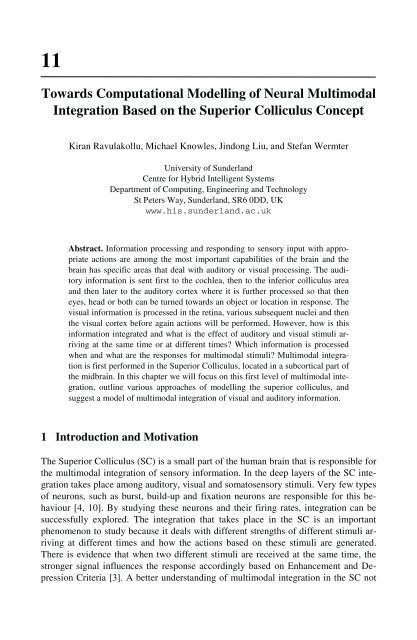
11<br />
<strong>Towards</strong> <strong>Computational</strong> <strong>Modelling</strong> <strong>of</strong> <strong>Neural</strong> <strong>Multimodal</strong><br />
<strong>Integration</strong> Based on the Superior Colliculus Concept<br />
Kiran Ravulakollu, Michael Knowles, Jindong Liu, and Stefan Wermter<br />
University <strong>of</strong> Sunderland<br />
Centre for Hybrid Intelligent Systems<br />
Department <strong>of</strong> Computing, Engineering and Technology<br />
St Peters Way, Sunderland, SR6 0DD, UK<br />
www.his.sunderland.ac.uk<br />
Abstract. Information processing and responding to sensory input with appropriate<br />
actions are among the most important capabilities <strong>of</strong> the brain and the<br />
brain has specific areas that deal with auditory or visual processing. The auditory<br />
information is sent first to the cochlea, then to the inferior colliculus area<br />
and then later to the auditory cortex where it is further processed so that then<br />
eyes, head or both can be turned towards an object or location in response. The<br />
visual information is processed in the retina, various subsequent nuclei and then<br />
the visual cortex before again actions will be performed. However, how is this<br />
information integrated and what is the effect <strong>of</strong> auditory and visual stimuli arriving<br />
at the same time or at different times? Which information is processed<br />
when and what are the responses for multimodal stimuli? <strong>Multimodal</strong> integration<br />
is first performed in the Superior Colliculus, located in a subcortical part <strong>of</strong><br />
the midbrain. In this chapter we will focus on this first level <strong>of</strong> multimodal integration,<br />
outline various approaches <strong>of</strong> modelling the superior colliculus, and<br />
suggest a model <strong>of</strong> multimodal integration <strong>of</strong> visual and auditory information.<br />
1 Introduction and Motivation<br />
The Superior Colliculus (SC) is a small part <strong>of</strong> the human brain that is responsible for<br />
the multimodal integration <strong>of</strong> sensory information. In the deep layers <strong>of</strong> the SC integration<br />
takes place among auditory, visual and somatosensory stimuli. Very few types<br />
<strong>of</strong> neurons, such as burst, build-up and fixation neurons are responsible for this behaviour<br />
[4, 10]. By studying these neurons and their firing rates, integration can be<br />
successfully explored. The integration that takes place in the SC is an important<br />
phenomenon to study because it deals with different strengths <strong>of</strong> different stimuli arriving<br />
at different times and how the actions based on these stimuli are generated.<br />
There is evidence that when two different stimuli are received at the same time, the<br />
stronger signal influences the response accordingly based on Enhancement and Depression<br />
Criteria [3]. A better understanding <strong>of</strong> multimodal integration in the SC not
2 K. Ravulakollu et al.<br />
only helps in exploring the properties <strong>of</strong> the brain, but also provides indications for<br />
building novel bio-inspired computational or robotics models.<br />
<strong>Multimodal</strong> integration allows humans and animals to perform under difficult, potentially<br />
noisy auditory or visual stimulus conditions. In the human brain, the Superior<br />
Colliculus is the first region that provides this multimodal integration [23]. The deep<br />
layers <strong>of</strong> the Superior Colliculus integrate multisensory inputs and generate directional<br />
information that can be used to identify the source <strong>of</strong> the input information<br />
[20]. The SC uses visual and auditory information for directing the eyes using saccades,<br />
that is horizontal eye movements which direct the eyes to the location <strong>of</strong> the<br />
object which generated the stimulus. Before integrating the different modalities the<br />
individual stimuli are preprocessed in separate auditory and visual pathways. Preprocessed<br />
visual and auditory stimuli can then be used to integrate the stimuli in the deep<br />
layers <strong>of</strong> the SC and eventually generate responses based on the multimodal input.<br />
The types <strong>of</strong> saccades can be classified in different ways [39] as shown in Figure 1.<br />
Most saccades are reflexive and try to identify the point <strong>of</strong> interest in the visual field<br />
which has moved due to the previous visual frame changing to the current one [20]. If<br />
no point <strong>of</strong> interest is found in the visual field, auditory information can be used to<br />
identify a source. Saccades are primary actions which in some cases are autonomous<br />
and are carried out without conscious processing in the brain. When there is insufficient<br />
information to determine the source based on a single modality, the SC uses<br />
multimodal integration to determine the output. Saccades are the first actions taken as<br />
a result <strong>of</strong> receiving enough visual and auditory stimuli.<br />
Saccades<br />
Reflexive<br />
Targeted<br />
Visual<br />
Range<br />
Visual &<br />
Auditory<br />
Visual<br />
Range<br />
Visual &<br />
Auditory<br />
Auditory<br />
Range<br />
Auditory<br />
Range<br />
Fig. 1. The different types <strong>of</strong> saccades that are executed by the eyes <strong>of</strong> a mammal<br />
It is known that the SC plays a significant role in the control <strong>of</strong> saccades and head<br />
movements [3, 23, 33]. In addition to the reflexive saccades, saccades can also be<br />
targeted on a particular object in the visual field. In this case, the SC receives the visual<br />
stimulus at its superficial layers which are mainly used to direct the saccades to<br />
any change in the visual field. In a complementary manner, the deep layers <strong>of</strong> the<br />
SC are capable <strong>of</strong> receiving auditory stimuli from the Inferior Colliculus and other
<strong>Towards</strong> <strong>Computational</strong> <strong>Modelling</strong> <strong>of</strong> <strong>Neural</strong> <strong>Multimodal</strong> <strong>Integration</strong> 3<br />
Visual & Auditory<br />
<strong>Integration</strong><br />
Depression<br />
Enhancement<br />
Fig. 2. Types <strong>of</strong> effects in multimodal integration after integrating the visual and auditory fields.<br />
cortical regions. The deep layers <strong>of</strong> the Superior Colliculus are also responsible for<br />
integrating multisensory inputs for the generation <strong>of</strong> actions. The SC is capable <strong>of</strong><br />
generating output even if the signal strength <strong>of</strong> a single modality would not be sufficient<br />
or too high to trigger an action (see Figure 2). The enhancement is increasing the<br />
relevance <strong>of</strong> a particular modality stimulus based on the influence <strong>of</strong> other modalities<br />
while depression is decreasing the relevance <strong>of</strong> a particular modality, in particular if<br />
the stimuli disagree.<br />
Several authors have attempted to examine multimodal integration in the Superior<br />
Colliculus [2, 4, 5, 10, 27, 37, 51, 55]. Different approaches have been suggested including<br />
biological, probabilistic and computational neural network approaches. Of<br />
the different researchers that pursued a probabilistic approach, Anastasio has made<br />
the assumption that SC neurons show inverse effectiveness. In related probabilistic<br />
research, Wilhelm et al used a Gaussian distribution function along with a preprocessing<br />
level for enhancement criteria in SC modelling. Other researchers like<br />
Maren and Dominik [30] and Mass et al [17] have used a probabilistic approach in<br />
conjunction with other extraction techniques for modelling multimodal integration for<br />
other applications.<br />
In contrast to probabilistic approaches, Trappenberg [48], Christian Quaia [4] and<br />
others have developed neural models <strong>of</strong> the SC. Christiano Cuppini [5] and Casey Pavlov<br />
[33] have also suggested a specific SC model but the model is based on many assumptions<br />
and only functions with specified input patterns. Also the enhancement and<br />
depression criteria are not comprehensively addressed. Yagnanarayana has used the<br />
concept <strong>of</strong> multimodal integration based on the superior colliculus and implemented it<br />
in various applications <strong>of</strong> an autoassociative neural network. According to J. Pavon<br />
[19], this multimodal integration concept is used to achieve efficiency in agents when<br />
co-operating and co-ordinating with various sensor data modalities. Similarly Rita<br />
Cucchiara [39] has established a biometric multimedia surveillance system that uses<br />
multimodal integration techniques for an effective surveillance system, but the multimodal<br />
usage is not able to overcome problems like the influence <strong>of</strong> noise.<br />
In summary, while probabilistic approaches <strong>of</strong>ten emphasise computational efficiency,<br />
the neural approach <strong>of</strong>fers a more realistic bio-inspired approach for modelling<br />
the Superior Colliculus. Therefore, in the next section our neural SC modelling<br />
methodology will be described followed by enhancement and depression modelling<br />
performed by the SC.
4 K. Ravulakollu et al.<br />
2 <strong>Towards</strong> a New Methodology and Architecture<br />
2.1 Overview <strong>of</strong> the Architecture and Environment<br />
The approach proposed in this section addresses the biological functionality <strong>of</strong> the SC<br />
in a computational model. Our approach mainly aims at generating an integrated response<br />
for auditory or visual signals. In this context, neural networks are particularly<br />
attractive for SC modelling because <strong>of</strong> their support <strong>of</strong> self organisation, feature map<br />
representations and association between the layers. Figure 3 gives an overview <strong>of</strong> our<br />
general layered architecture. Hence a two-layer neural network is considered where<br />
each layer receives inputs from different auditory and visual stimuli, and integrates<br />
these inputs in a synchronised manner to produce the output.<br />
Auditory<br />
Visual<br />
Associative Mapping<br />
Multisensory<br />
Integrated<br />
Fig. 3. A layered neural network capable <strong>of</strong> processing inputs from both input layers. <strong>Integration</strong><br />
is carried out by an associative mapping.<br />
For auditory input data processing, the Time Difference <strong>of</strong> Arrival (TDOA) is calculated<br />
and projected on the auditory layer. The auditory input is provided to the<br />
model in the form <strong>of</strong> audible sound signals within the range <strong>of</strong> the microphones. Similarly<br />
for visual input processing, a difference image, DImg, is calculated from the<br />
current and previous visual frames and is projected on the visual layer. Both visual<br />
and auditory input is received by the network as real time input stimuli. These stimuli<br />
are used to determine the source <strong>of</strong> the visual or auditory stimuli. Then the auditory<br />
and visual layers are associated for the generation <strong>of</strong> the integrated output. In case <strong>of</strong><br />
the absence <strong>of</strong> one <strong>of</strong> the two inputs, the final decision on the direction <strong>of</strong> the saccade<br />
is made based only on the present input stimuli. In the case <strong>of</strong> simultaneous arrival <strong>of</strong><br />
different sensory inputs, the model integrates both inputs and generates a common<br />
enhanced or depressed output, depending on the signal strength <strong>of</strong> the inputs. Our<br />
particular focus is on studying the appropriate depression and enhancement processes.
<strong>Towards</strong> <strong>Computational</strong> <strong>Modelling</strong> <strong>of</strong> <strong>Neural</strong> <strong>Multimodal</strong> <strong>Integration</strong> 5<br />
For evaluating our methodology we base our evaluation on the behavioural framework<br />
<strong>of</strong> Stein and Meredith [3]. Stein and Meredith’s experiments are carried out<br />
examining a cat’s superior colliculus using a neuro-biological/behavioural methodology<br />
to test hypotheses in neuroscience. This experimental setup provides a good<br />
starting point for carrying out our series <strong>of</strong> experiments. Our environment includes a<br />
series <strong>of</strong> auditory sources like speakers and visual sources like LEDs arranged as a<br />
semicircular environment so that each source will have the same distance from the<br />
centre covering 180 degrees <strong>of</strong> visual and auditory ranges.<br />
For the model demonstration, Stein and Meredith’s behavioural setup is modified<br />
by replacing the cat with a robot head as shown in Figure 4. As a result <strong>of</strong> visual or<br />
auditory input the robot’s head is turned towards the direction <strong>of</strong> the source. The advantages<br />
<strong>of</strong> using this environment are that environmental noise can be considered<br />
during detecting and tracking and the enhancement and depression phenomena can be<br />
studied.<br />
LED<br />
Fig. 4. Experimental setup and robot platform for testing the multimodal integration model for<br />
an agent based on visual and auditory stimuli<br />
2.2 Auditory Data Processing<br />
The first set <strong>of</strong> experiments is based on collecting the auditory data from a tracking<br />
system within our experimental platform setup. We can determine the auditory sound<br />
source using the interaural time difference for two microphones [31] and the TDOA<br />
(Time Difference Of Arrival), which is used for calculating the distance from the<br />
sound source to the agent. The signal overlap <strong>of</strong> the left and right stimuli allows determining<br />
the time difference.<br />
( xcorr( L,<br />
R)<br />
)<br />
length<br />
+ 1<br />
<br />
TDOA = <br />
− max , ×<br />
2<br />
<br />
( xcorr( L R)<br />
) Sr
6 K. Ravulakollu et al.<br />
In the above equation ‘xcorr ()’ is the function that determines the cross-correlation<br />
<strong>of</strong> the left ‘L’ and right ‘R’ channels <strong>of</strong> a sound signal. S r stands for sample rate <strong>of</strong> the<br />
sound card used by the agent. Once the time difference <strong>of</strong> arrival is determined the<br />
distance <strong>of</strong> the sound source from the agent is calculated using the following:<br />
Distance=TDOA x sound frequency<br />
The result is a vector map for further processing to generate the multimodal integrated<br />
output. However, for unimodal data sets, we can determine the direction <strong>of</strong> the<br />
sound source in a simplified manner using geometry and the data available including<br />
speed <strong>of</strong> sound and distance between the ears <strong>of</strong> the agent that is shown in the circular<br />
diagram below.<br />
η<br />
c<br />
α<br />
θ<br />
λ<br />
γ<br />
β<br />
Fig. 5. Determination <strong>of</strong> sound source directions using TDOA where c is the distance <strong>of</strong> the<br />
source and is the angle to be determined based on TDOA and the speed <strong>of</strong> sound. The distance<br />
d between two microphones, L and R, is known.<br />
Assume the sound source is in far-field, i.e. c>>d, then ==90 degree and the<br />
sound source direction can be calculated using triangulation as follows:<br />
==arcsine(ML/d)=arcsine(TDOA*Vs/d)<br />
where Vs is the sound speed in air.<br />
From the above methodology the unimodal data for the auditory input is collected<br />
and the auditory stimuli can be made available for the integration model.<br />
2.3 Visual Data Processing<br />
We now consider visual data processing where simple activated LEDs represent the<br />
location <strong>of</strong> the visual stimulus in the environment. A change in the environment is
<strong>Towards</strong> <strong>Computational</strong> <strong>Modelling</strong> <strong>of</strong> <strong>Neural</strong> <strong>Multimodal</strong> <strong>Integration</strong> 7<br />
determined based on the difference between subsequent images. By using a difference<br />
function, the difference between the two successive frames is calculated.<br />
DImg = abs_image_difference(image(i), image(i – 1))<br />
Once the difference images are obtained containing only the variations <strong>of</strong> the light<br />
intensity, they are transformed into a vector. Once the vectors are extracted they can<br />
be used as direct inputs to the integrated neural model. However, in the case <strong>of</strong> unimodal<br />
data, difference images (DImg) are processed directly to identify the area <strong>of</strong><br />
interest. The intensity <strong>of</strong> the light is also considered to identity an LED with larger<br />
brightness. Using this method a series <strong>of</strong> images is collected. From this vector the<br />
maximum color intensity location (maxindex) is identified and extracted. Using this<br />
information and the distance between the centre <strong>of</strong> the eyes to the visual aid, it is easy<br />
to determine the direction <strong>of</strong> the visual intensity changes in the environment using the<br />
following formula:<br />
( maxindex − half_visual_width)<br />
− × visual_range<br />
θ = tan 1<br />
<br />
<br />
visual_width x distance_<strong>of</strong>_sensor_to_source <br />
After running this experiment based on a set <strong>of</strong> 5 LEDs the different difference<br />
images were collected. By transforming the image on a 180 degree horizontal map<br />
with 5 degree intervals, the angle <strong>of</strong> the source is identified. For the data collected in<br />
the visual environment, 85 – 95 % accuracy is achieved for single stimulus inputs,<br />
and 79 – 85% accuracy is observed for multiple stimuli.<br />
Later during the integration, the signal strength is also included in the network for<br />
generating the output. Stein and Meredith have previously identified two phenomena,<br />
Difference Image (DImg)<br />
<br />
Camera<br />
Fig. 6. Difference Image (DImg) used for scaling and to determine the location <strong>of</strong> the highlighted<br />
area <strong>of</strong> the image in which the dash line represents the length <strong>of</strong> the visual range and<br />
distance between the two cameras
8 K. Ravulakollu et al.<br />
depression and enhancement, as crucial for multimodal integration. In our approach<br />
we have also considered the visual constraints from the consecutive frames for confirming<br />
whether a signal <strong>of</strong> low strength is a noise signal or not. By reducing the auditory<br />
frequency to 100Hz for a weak auditory signal and by also reducing the LEDs in<br />
the behavioural environment we are able to generate a weak stimulus to study the<br />
enhancement response.<br />
3 Simplified <strong>Modelling</strong> <strong>of</strong> the Superior Colliculus<br />
3.1 Unimodal Experiments<br />
First, unimodal data from auditory and visual stimuli are collected and the desired<br />
result is estimated to serve as comparison data for the integrated model. The agent is a<br />
0.2<br />
Left Channel<br />
0<br />
-0.2<br />
0.2<br />
0.123 0.124 0.125 0.126 0.127 0.128 0.129 0.13 0.131<br />
Right Channel<br />
0<br />
-0.2<br />
0.122 0.123 0.124 0.125 0.126 0.127 0.128 0.129 0.13 0.131<br />
1<br />
Sound Source Localization<br />
0.5<br />
0<br />
-80 -60 -40 -20 0 20 40 60 80<br />
(a)<br />
0.<br />
2<br />
0<br />
Left<br />
Channel<br />
-0.2<br />
0.122 0.123 0.124 0.125 0.126 0.127 0.128 0.129 0.13 0.131<br />
Right Channel<br />
0.<br />
2<br />
0<br />
-0.2<br />
0.122 0.123 0.124 0.125 0.126 0.127 0.128 0.129 0.13 0.131<br />
1<br />
Sound Source Localization<br />
0.5<br />
0<br />
-80 -60 -40 -20 0 20 40 60 80<br />
(b)<br />
Fig. 7. Graphical representation <strong>of</strong> auditory localization. The behavioural environment when<br />
there are two auditory inputs. The signal received at the left and right microphone are plotted<br />
on a graph with time on the x-axis and amplitude on the y-axis. Once the TDOA is calculated<br />
and the direction <strong>of</strong> the auditory source is located it can be shown in the range from -90 to 90<br />
degrees which in this case is identified as (a) 18 degree and (b) -10 degrees.
<strong>Towards</strong> <strong>Computational</strong> <strong>Modelling</strong> <strong>of</strong> <strong>Neural</strong> <strong>Multimodal</strong> <strong>Integration</strong> 9<br />
PeopleBot robot with a set <strong>of</strong> two microphones for auditory input and a camera for<br />
visual input.<br />
3.1.1 Auditory Experiments<br />
The agent used for auditory data collection has two microphones attached on either<br />
side <strong>of</strong> the head resembling ears. The speakers are stimulated using an external amplifier<br />
to generate sound signals <strong>of</strong> strength within human audible limits. For these experiments<br />
the signal levels <strong>of</strong> smaller frequencies are considered, since with these<br />
lower frequencies the multimodal behaviour can be identified and the behaviour can<br />
be studied at a more critical precision. Hence the frequencies with a range <strong>of</strong> 100 Hz -<br />
2K Hz are used. Sound stimuli are generated randomly from any <strong>of</strong> the different<br />
speakers, and by implementing the interaural time difference method from above, the<br />
direction <strong>of</strong> the stimulus is determined. The following table provide example results<br />
<strong>of</strong> these auditory experiments <strong>of</strong> various directions and stimuli levels.<br />
By running the above experiment for lower frequency ranges <strong>of</strong> 100 to 500 Hz<br />
with the amplitude level at 8 (as the recognition is effective at this level), initial experiments<br />
were carried out and the results are presented below. For each frequency<br />
from 100Hz, the sound stimuli are activated at angles varying from -90 to 90 degrees.<br />
Below in table 1 we show the angles computed by the tracking system discussed in<br />
the above section.<br />
Table 1. This table depicts the accuracy level <strong>of</strong> the various frequencies from 100Hz to 500Hz.<br />
Actual Angle<br />
Freq. vs -90 -60 -45 -30 -20 -10 0 10 20 30 45 60 90<br />
Angle<br />
100 -81.07 -61.39 -6.29 -31.44 -21.41 -8.4 0 10.52 21.41 33.97 41.07 63.39 50.04<br />
200 -71.07 -63.39 -42.11 -33.97 -25.97 -14.8 0 10.52 21.41 35.59 42.11 63.69 80.2<br />
300 -76.88 -63.39 -41.07 -29.97 -25.97 -14.8 -2.09 12.4 21.41 31.44 38.95 63.39 80.00<br />
400 -73.19 -63.39 -41.07 -75.6 -33.41 -10.52 -2.09 10.42 16.98 36.59 41.07 63.39 73.41<br />
500 -43.9 -63.4 -17 -22.14 -17 -10.5 0 10.52 21.41 29.29 48.4 63.39 53.41<br />
3.1.2 Visual Experiments<br />
The camera is directed to cover 120 degrees, from -60 to 60. The series <strong>of</strong> frames<br />
collected as input from the camera are processed and the output should determine<br />
which <strong>of</strong> the LEDs is active. The frames that are captured from the camera are used to<br />
produce the difference image (DImg) which contains only the changes that have occurred<br />
in the visual environment <strong>of</strong> the agent. These difference images are calculated<br />
by measuring the RGB intensity variations from pixel to pixel in the two successive<br />
images.<br />
Below we show how these difference images are generated based on two successive<br />
frames where the first frame is a null image with no activation and the second<br />
frame has activation at two different locations. The third image is the difference
10 K. Ravulakollu et al.<br />
(a) (b) (c)<br />
Fig. 8. (a) The visual environment without visual LED stimulus (b) The environment with visual<br />
LED stimulus. (c) The difference image (DImg).<br />
image generated from the first two frames. This series <strong>of</strong> difference images is used to<br />
identify change in the environment. The difference images can be plotted on a plane<br />
covering -90 to 90 degrees on a special scale to intensity values <strong>of</strong> the difference<br />
image signal strength. The following image represents one such plotting <strong>of</strong> the difference<br />
image signal intensity.<br />
Using this plot, the direction <strong>of</strong> the source from the centre <strong>of</strong> the agent is determined.<br />
The difference images are mapped on to a standard Horizontal Scale Frame (HSFr), to<br />
determine the location <strong>of</strong> the activation. The HSFr is a scale that divides the 180 degrees<br />
with 5 degrees <strong>of</strong> freedom. This scale image is different for different images.<br />
In this horizontal scale frame the horizontal axis is divided into 10 degree intervals.<br />
Hence all the visual information that arrives at the camera <strong>of</strong> the agent is transformed<br />
into a difference image intensity plot and finally plotted on an HSFr to locate the<br />
source in the visual environment. Within this process, different auditory and visual<br />
inputs are collected and later used as a test set for the neural network that can generate<br />
multimodal integrated output for the similar auditory and visual inputs.<br />
A synchronous timer is used to verify and confirm whether the visual and auditory<br />
stimuli are synchronized in terms <strong>of</strong> time <strong>of</strong> arrival (TOA). If the arrival <strong>of</strong> the stimuli<br />
is asynchronous then an integration <strong>of</strong> the inputs is not necessary, as the location <strong>of</strong><br />
the source can be determined depending on the unimodal processing. In cases <strong>of</strong> multiple<br />
signals with a synchronous TOA, the signal strength is considered for both signals.<br />
Once the strongest signal is identified then the preference is given first to this<br />
signal and only later an additional preference may be associated with the other signal.<br />
This case occurs mainly with unimodal data such as a visual environment with two<br />
different visual stimuli or an auditory field with two different stimuli.<br />
3.2 <strong>Multimodal</strong> Experiments<br />
Now we focus on the combination <strong>of</strong> both auditory and visual processing as shown in<br />
Figure 4. The received auditory and visual inputs are preprocessed considering<br />
the functionality <strong>of</strong> the optic chiasm and the information flow in the optic tract. This
<strong>Towards</strong> <strong>Computational</strong> <strong>Modelling</strong> <strong>of</strong> <strong>Neural</strong> <strong>Multimodal</strong> <strong>Integration</strong> 11<br />
Difference Image<br />
300<br />
200<br />
100<br />
0<br />
0 50 100 150 200 250 300 350<br />
1<br />
Visual Source Localization<br />
0.5<br />
0<br />
-80 -60 -40 -20 0 20 40 60 80<br />
Fig. 9. (a) The difference image (DImg) is shown scaled to a unique size for all the images to<br />
standardize as a vector for the map alignment in the multimodal phase. (b) Horizontal Scale<br />
Frame image (HSFr) is a frame scale which is scaled to -90 to 90 degrees used as a reference to<br />
check in which block the enlightened part <strong>of</strong> the difference image falls.<br />
Visual<br />
Stimulus<br />
Auditory<br />
Stim<br />
DImg<br />
TDOA<br />
SC<br />
Fig. 10. Schematic representation <strong>of</strong> stimuli flow from the external environment to the superior<br />
colliculus model
12 K. Ravulakollu et al.<br />
preprocessing generates the difference image (DImg) from the captured visual input<br />
and the time difference <strong>of</strong> arrival (TDOA) for the auditory stimulus as shown in<br />
Figure 10. The preprocessed information enters the network which performs multimodal<br />
integration <strong>of</strong> the available stimulus and a corresponding output is generated.<br />
The network model is mainly focused on map alignment to resemble the actual integration<br />
in the deep layers <strong>of</strong> the Superior Colliculus. In this network two types <strong>of</strong><br />
inputs are considered: the TDOA auditory map and the DImg visual stimulus map are<br />
used for the integration. The TDOA is converted into a vector <strong>of</strong> specific size which<br />
in this case is 10 by 320 containing the information <strong>of</strong> the waveform with the intensities<br />
<strong>of</strong> the input signal. Similarly the difference image is converted into a vector <strong>of</strong><br />
similar size containing only the information <strong>of</strong> horizontal intensity variations in the<br />
difference image.<br />
These two vector representations are the input for the multimodal integration<br />
model. Since we are focussing on horizontal saccades, only the variations at a horizontal<br />
scale are considered at this point although this can be extended to vertical<br />
saccades. To identify the highest <strong>of</strong> multiple stimuli, a Bayesian probability-based<br />
approach is used to determine the signal strength as input to the network. A synchronous<br />
timer is used for counting the time that lapses between the arrival <strong>of</strong> the various<br />
stimuli <strong>of</strong> the corresponding senses.<br />
The integration model is a two-layer neural network with the size 10 by 32 based<br />
on the size <strong>of</strong> the input images generated. Hence for the integration in the network the<br />
weighted average is considered as follows:<br />
Integrated Output = ((W V * V 1 ) + (W A * A 1 ))/(W V + W A )<br />
where W v = Visual Vector Weight, W A = Auditory Vector Weight, V 1 = normalised<br />
Visual Vector and A 1 = normalised Auditory Vector.<br />
This weight function determines the weighted location <strong>of</strong> the source and provides a<br />
degree value where the source is. The difference between the two will allow the<br />
model to determine the stronger source.<br />
<strong>Integration</strong> Case Studies:<br />
• Multiple visual input stimuli: In case <strong>of</strong> more than one visual input in the<br />
environment, the difference image is generated highlighting the areas <strong>of</strong> visual<br />
interference. From the difference image the intensity <strong>of</strong> the signal is identified<br />
in terms <strong>of</strong> RGB values as shown below in figure 11. Examining the first and<br />
last spike shows that the green spike is low in intensity compared to the second<br />
one. Considering the second, the green and red spikes are high in the intensity<br />
when compared to the rest. However, the plot <strong>of</strong> the maximum values <strong>of</strong> the<br />
available RGB intensities determines the position <strong>of</strong> the source. By plotting the<br />
position onto a [-90, 90] scale the location <strong>of</strong> the source is determined, which<br />
in this example case in figure 11 is -30.
<strong>Towards</strong> <strong>Computational</strong> <strong>Modelling</strong> <strong>of</strong> <strong>Neural</strong> <strong>Multimodal</strong> <strong>Integration</strong> 13<br />
Difference Image<br />
300<br />
200<br />
100<br />
0<br />
0 50 100 150 200 250 300 350<br />
1<br />
Visual Source Localization<br />
0.5<br />
0<br />
-80 -60 -40 -20 0 20 40 60 80<br />
Fig. 11. The figure depicts multiple visual input stimuli received by the agent and how the visual<br />
localization is determined using the difference image and intensity plotting. The maximum<br />
intensity is identified in the second peak where all RGB values are highest when compared with<br />
the rest <strong>of</strong> the peaks.<br />
If there are even more visual stimuli, the behaviour <strong>of</strong> our model is similar, and it<br />
calculates the intensities <strong>of</strong> the signals and plots the maximum <strong>of</strong> them in the standard<br />
plotting area [-90, 90]. In this case a close inspection <strong>of</strong> the spikes reveals the small<br />
difference that is present in the green spikes <strong>of</strong> each stimulus spike.<br />
• Low auditory and strong visual stimuli: If a low intensity auditory signal and<br />
a visual signal with strong intensity value are received at the same time as input<br />
to the multimodal integration system, after verifying the time frame to confirm<br />
the arrival <strong>of</strong> the signals, both inputs are considered. After preprocessing <strong>of</strong> the<br />
signals, the signal maps are generated. In the graphs we can observe that the<br />
signal in the auditory plot has a very low intensity and the angle is determined.<br />
For the visual stimulus, the single spikes in red and green are considered for the<br />
maximum signal value. When plotted on the standard space scale, the source<br />
locations are identified as two different locations but the overall integrated location<br />
is identified as being close to the stronger visual stimulus.
14 K. Ravulakollu et al.<br />
300<br />
200<br />
100<br />
0<br />
0 50 100 150 200 250 300 350<br />
1<br />
Visual Source Localization<br />
0.5<br />
0<br />
-80 -60 -40 -20 0 20 40 60 80<br />
Fig. 12. The figure depicts multiple visual stimuli and how the model deals with such<br />
input. The plot shows the maximum intensity peak location and how the preferred location is<br />
determined.<br />
• Strong Auditory and Low Visual Stimuli: In this case the intensity <strong>of</strong> the<br />
auditory signal is strong and the intensity <strong>of</strong> visual signal is low. For the visual<br />
stimulus, the strength <strong>of</strong> the green spikes is similar for both activation cases,<br />
while the red spikes vary. Determining the location <strong>of</strong> the two inputs individually,<br />
the locations are on different sides <strong>of</strong> the centre. When the multimodal<br />
output is generated, the location <strong>of</strong> the integrated output is close towards the<br />
auditory stronger stimulus.<br />
The above two representative cases are observed during multimodal integration<br />
with one <strong>of</strong> the signals being very strong in its intensity. The Superior Colliculus<br />
model focuses on the stimulus with the highest intensity and therefore the integrated<br />
decision is influenced by one <strong>of</strong> the stimuli.<br />
• Strong visual and strong auditory stimuli: In this case scenario, when the<br />
signals are received by the sensors, the signal intensities are calculated and the<br />
modalities are plotted on an intensity graph to determine the signal intensity. In<br />
the intensity graphs shown, the sources are located at either side <strong>of</strong> the centre<br />
and the activations are <strong>of</strong> high intensities. When the output is computed, the<br />
source is located close to the visually detected peak since the visual stimulus<br />
has greater priority than the auditory stimulus.
<strong>Towards</strong> <strong>Computational</strong> <strong>Modelling</strong> <strong>of</strong> <strong>Neural</strong> <strong>Multimodal</strong> <strong>Integration</strong> 15<br />
0.2<br />
Left Channel<br />
0<br />
-0.2<br />
0.122 0.124 0.126 0.128 0.13 0.132<br />
0.2<br />
Right Channel<br />
0<br />
-0.2<br />
0.122 0.124 0.126 0.128 0.13 0.132<br />
1<br />
Sound Source Localization<br />
0.5<br />
0<br />
-80 -60 -40 -20 0 20 40 60 80<br />
300<br />
200<br />
100<br />
0<br />
0 50 100 150 200 250 300 350<br />
1<br />
Visual Source Localization<br />
0.5<br />
0<br />
-80 -60 -40 -20 0 20 40 60 80<br />
1<br />
Integrated source localization<br />
0.5<br />
0<br />
-80 -60 -40 -20 0 20 40 60 80<br />
Fig. 13. Auditory and visual input with strong visual stimulus determining the main preference<br />
for the localization.
16 K. Ravulakollu et al.<br />
0.2<br />
Left Channel<br />
0<br />
-0.2<br />
0.122 0.123 0.124 0.125 0.126 0.127 0.128 0.129 0.13 0.131<br />
0.2<br />
Right Channel<br />
0<br />
-0.2<br />
0.122 0.123 0.124 0.125 0.126 0.127 0.128 0.129 0.13 0.131<br />
1<br />
Sound Source Localization<br />
0.5<br />
0<br />
-80 -60 -40 -20 0 20 40 60 80<br />
200<br />
150<br />
100<br />
50<br />
0<br />
0 50 100 150 200 250 300 350<br />
1<br />
Visual Source Localization<br />
0.5<br />
0<br />
-80 -60 -40 -20 0 20 40 60 80<br />
1<br />
Integrated Source Localization<br />
0.5<br />
0<br />
-80 -60 -40 -20 0 20 40 60 80<br />
Fig. 14. <strong>Multimodal</strong> input case with strong auditory stimulus. The integrated output is biased<br />
by the intensity <strong>of</strong> the stronger stimulus which in this case is auditory.<br />
It is not clear whether the superior colliculus will prioritize in every case, but in the<br />
case <strong>of</strong> multiple strong intensity stimuli the visual stimulus will have the higher priority<br />
while the strong auditory stimulus will have some influence on the multimodal<br />
integrated output.
<strong>Towards</strong> <strong>Computational</strong> <strong>Modelling</strong> <strong>of</strong> <strong>Neural</strong> <strong>Multimodal</strong> <strong>Integration</strong> 17<br />
300<br />
200<br />
100<br />
0<br />
0 50 100 150 200 250 300 350<br />
1<br />
Visual Source Localization<br />
0.5<br />
0<br />
-80 -60 -40 -20 0 20 40 60 80<br />
0.2<br />
Left Channel<br />
0<br />
-0.2<br />
0.122 0.123 0.124 0.125 0.126 0.127 0.128 0.129 0.13 0.131<br />
0.2<br />
Right Channel<br />
0<br />
-0.2<br />
0.122 0.123 0.124 0.125 0.126 0.127 0.128 0.129 0.13 0.131<br />
1<br />
Sound Source Localization<br />
0.5<br />
0<br />
-80 -60 -40 -20 0 20 40 60 80<br />
1<br />
Integrated Source Localization<br />
0.5<br />
0<br />
-80 -60 -40 -20 0 20 40 60 80<br />
Fig. 15. <strong>Multimodal</strong> enhancement response: The integrated output is generated based on a<br />
distance function between the auditory and visual intensity.
18 K. Ravulakollu et al.<br />
200<br />
150<br />
100<br />
50<br />
0<br />
0 50 100 150 200 250 300 350<br />
1<br />
Visual Source Localization<br />
0.5<br />
0<br />
-80 -60 -40 -20 0 20 40 60 80<br />
0.2<br />
Left Channel<br />
0<br />
-0.2<br />
0.122 0.123 0.124 0.125 0.126 0.127 0.128 0.129 0.13 0.131<br />
0.2<br />
Right Channel<br />
0<br />
-0.2<br />
0.122 0.123 0.124 0.125 0.126 0.127 0.128 0.129 0.13 0.131<br />
1<br />
Sound Source Localization<br />
0.5<br />
0<br />
-80 -60 -40 -20 0 20 40 60 80<br />
1<br />
Integrated source localization<br />
0.5<br />
0<br />
-80 -60 -40 -20 0 20 40 60 80<br />
Fig. 16. <strong>Multimodal</strong> depression response: The integrated output is generated based on a distance<br />
function between the auditory and visual intensity where the auditory signal is suppressed<br />
due to its low intensity and the visual stimulus is the only input available. Hence the distance<br />
function is biased towards the visual stimulus.
<strong>Towards</strong> <strong>Computational</strong> <strong>Modelling</strong> <strong>of</strong> <strong>Neural</strong> <strong>Multimodal</strong> <strong>Integration</strong> 19<br />
300<br />
200<br />
100<br />
0<br />
0 50 100 150 200 250 300 350<br />
1<br />
Visual Source Localization<br />
0.5<br />
0<br />
-80 -60 -40 -20 0 20 40 60 80<br />
0.2<br />
Left Channel<br />
0<br />
-0.2<br />
0.122 0.123 0.124 0.125 0.126 0.127 0.128 0.129 0.13 0.131<br />
0.2<br />
Right Channel<br />
0<br />
-0.2<br />
0.122 0.123 0.124 0.125 0.126 0.127 0.128 0.129 0.13 0.131<br />
1<br />
Sound Source Localization<br />
0.5<br />
0<br />
-80 -60 -40 -20 0 20 40 60 80<br />
1<br />
Integrated source localization<br />
0.5<br />
0<br />
-80 -60 -40 -20 0 20 40 60 80<br />
Fig. 17. <strong>Multimodal</strong> Depression Responses: a weak or low intensity auditory signal has<br />
suppressed the total multimodal response and generated a new signal that can achieve the response<br />
accurately but with a very low signal strength. This phenomenon is observed once in<br />
twenty responses, as in the remaining cases, the model tries to classify the stimuli to generate<br />
the output.
20 K. Ravulakollu et al.<br />
• Low visual and low auditory: In circumstances where both visual and auditory<br />
signals are <strong>of</strong> low intensities, the behaviour <strong>of</strong> the superior colliculus is<br />
<strong>of</strong>ten difficult to predict and determine. In this case, the superior colliculus can<br />
be thought <strong>of</strong> as a kind <strong>of</strong> search engine that keeps traversing the environment<br />
to locate any variations in the environment. When both auditory and visual<br />
signals are <strong>of</strong> low intensity, the SC suppresses the auditory signal due to its<br />
low intensity. Though the visual signal is low in its intensity, as far as the SC<br />
is concerned, it is the only sensory data available. Therefore, the source is<br />
identified much closer to the visual stimulus as shown in figure 16 below.<br />
In some cases, if the stimulus is not in the range <strong>of</strong> [-30, 30] degrees, depression<br />
may occur if the visual stimulus is getting out <strong>of</strong> range or the auditory stimulus is getting<br />
less intense.<br />
4 Summary and Conclusion<br />
We have discussed a model <strong>of</strong> the SC in the context <strong>of</strong> evaluating the state <strong>of</strong> art in<br />
multimodal integration based on the SC. A neural computational model <strong>of</strong> the subcortical<br />
Superior Colliculus is being designed to demonstrate the multimodal integration<br />
that is performed in the deep layers. The enhancement and depression phenomena<br />
with low signal strength are demonstrated and the impact <strong>of</strong> multimodal integration<br />
is discussed. The presented model provides a first insight into the computational modeling<br />
and performance <strong>of</strong> the SC based on the concepts <strong>of</strong> Stein and Meredith and<br />
highlights the generated multimodal output. This work indicates a lot <strong>of</strong> potential for<br />
subsequent research for the model to emerge as a full computational multimodal sensory<br />
data integration model <strong>of</strong> the Superior Colliculus.<br />
Acknowledgements<br />
The authors extend their gratitude to Chris Rowan and Eric Hill for the assistance in<br />
setting up the experimental environment.<br />
References<br />
1. Green, A., Eklundh, K.S.: Designing for Learnability in Human-Robot Communication.<br />
IEEE Transactions on Industrial Electronics 50(4), 644–650 (2003)<br />
2. Arai, K., Keller, E.L., Edelman, J.A.: A <strong>Neural</strong> Network Model <strong>of</strong> Saccade Generation Using<br />
Distributed Dynamic Feedback to Superior Colliculus. In: Proceedings <strong>of</strong> International<br />
Joint Conference on <strong>Neural</strong> Networks, pp. 53–56 (1993)<br />
3. Stein, B.E., Meredith, M.A.: The Merging <strong>of</strong> the Senses. Cognitive Neuroscience Series.<br />
MIT Press, Cambridge (1993)<br />
4. Quaia, C., Lefevre, P., Optican, L.M.: Model <strong>of</strong> the Control <strong>of</strong> Saccades by Superior Colliculus<br />
and Cerebellum. Journal <strong>of</strong> Neurophysiology 82(2), 999–1018 (1999)<br />
5. Cuppini, C., Magosso, E., Serino, A., Pellegrino, G.D., Ursino, M.: A <strong>Neural</strong> Network for<br />
the Analysis <strong>of</strong> Multisensory <strong>Integration</strong> in the Superior Colliculus. In: de Sá, J.M., Alexandre,<br />
L.A., Duch, W., Mandic, D.P. (eds.) ICANN 2007, Part II. LNCS, vol. 4669, pp. 9–<br />
11. Springer, Heidelberg (2007)
<strong>Towards</strong> <strong>Computational</strong> <strong>Modelling</strong> <strong>of</strong> <strong>Neural</strong> <strong>Multimodal</strong> <strong>Integration</strong> 21<br />
6. Gilbert, C., Kuenen, L.P.S.: <strong>Multimodal</strong> <strong>Integration</strong>: Visual Cues Help Odour-Seeking<br />
Fruit Flies. Current Biology 18, 295–297 (2008)<br />
7. Fitzpatrick, D.C., Kuwada, S., Batra, R.: Transformations in processing Interaural time difference<br />
between the superior olivary complex and inferior colliculus: beyond Jeffress<br />
model. Hearing Research 168, 79–89 (2002)<br />
8. Massaro, D.W.: A Framework for Evaluating <strong>Multimodal</strong> integration by Humans and A<br />
Role for Embodied Conversational Agents. In: Proceedings <strong>of</strong> the 6th International Conference<br />
on <strong>Multimodal</strong> Interfaces (ICMI 2004), pp. 24–31 (2004)<br />
9. Droulez, J., Berthoz, A.: A neural network model <strong>of</strong> sensoritopic maps with predictive<br />
short-term memory properties. In: Proceedings <strong>of</strong> the National Academy <strong>of</strong> Sciences,<br />
USA, Neurobiology, vol. 88, pp. 9653–9657 (1991)<br />
10. Girard, B., Berthoz, A.: From brainstem to cortex: <strong>Computational</strong> models <strong>of</strong> saccade generation<br />
circuitry. Progress in Neurobiology 77, 215–251 (2005)<br />
11. Gurney, K.: Integrative computation for autonomous agents: a novel approach based on<br />
the vertebrate brain. Talk presented at EPSRC Novel computation initiative meeting<br />
(2003)<br />
12. Yavuz, H.: An integrated approach to the conceptual design and development <strong>of</strong> an intelligent<br />
autonomous mobile robot. Robotics and Autonomous Systems 55, 498–512 (2007)<br />
13. Hanheide, M., Bauckhage, C., Sagerer, G.: Combining Environmental Cues & Head Gestures<br />
to Interact with Wearable Devices. In: Proceedings <strong>of</strong> 7th International Conference<br />
on <strong>Multimodal</strong> Interfaces, pp. 25–31 (2005)<br />
14. Laubrock, J., Engbert, R., Kliegl, R.: Fixational eye movements predict the perceived direction<br />
<strong>of</strong> ambiguous apparent motion. Journal <strong>of</strong> Vision 8(14), 1–17 (2008)<br />
15. Lewald, J., Ehrenstein, W.H., Guski, R.: Spatio-temporal constraints for auditory-visual integration.<br />
Behavioural Brain Research 121(1-2), 69–79 (2001)<br />
16. Wolf, J.C., Bugmann, G.: Linking Speech and Gesture in <strong>Multimodal</strong> Instruction Systems.<br />
In: The 15th IEEE International Symposium on Robot and Human Interactive Communication<br />
(RO-MAN 2006), UK (2006)<br />
17. Maas, J.F., Spexard, T., Fritsch, J., Wrede, B., Sagerer, G.: BIRON, What’s the topic? – A<br />
Multi-Modal Topic Tracker for improved Human-Robot Interaction. In: The 15th IEEE International<br />
Symposium on Robot and Human Interactive Communication (RO-MAN<br />
2006), UK (2006)<br />
18. Armingol, J.M., del la Escalera, A., Hilario, C., Collado, J.M., Carrasco, J.P., Flores, M.J.,<br />
Postor, J.M., Rodriguez, F.J.: IVVI: Intelligent vehicle based on visual information. Robotics<br />
and Autonomous Systems 55, 904–916 (2007)<br />
19. Pavon, J., Gomez-Sanz, J., Fernandez-Caballero, A., Valencia-Jimenez, J.J.: Development<br />
<strong>of</strong> intelligent multisensor surveillance systems with agents. Robotics and Autonomous<br />
Systems 55, 892–903 (2007)<br />
20. Juan, C.H., Muggleton, N.G., Tzeng, O.J.L., Hung, D.L., Cowey, A., Walsh, V.: Segregation<br />
<strong>of</strong> Visual Selection and Saccades in Human. Cerebral Cortex 18(10), 2410–2415<br />
(2008)<br />
21. Groh, J.: Sight, sound processed together and earlier than previously thought, 919-660-<br />
1309, Duke University Medical Centre (2007) (Released, 29 October 2007)<br />
22. Jolly, K.G., Ravindran, K.P., Vijayakumar, R., Sreerama Kumar, R.: Intelligent decision<br />
making in multi-agent robot soccer system through compounded artificial neural networks.<br />
Robotics and Autonomous Systems 55, 589–596 (2006)<br />
23. King, A.J.: The Superior Colliculus. Current Biology 14(9), R335–R338 (2004)<br />
24. Kohonen, T.: Self-Organized formation <strong>of</strong> Topographical correct feature Maps. Biological<br />
Cybernetics 43, 59–69 (1982)
22 K. Ravulakollu et al.<br />
25. Voutsas, K., Adamy, J.: A Biologically inspired spiking neural network for sound source<br />
lateralization. IEEE transactions on <strong>Neural</strong> Networks 18(6), 1785–1799 (2007)<br />
26. Calms, L., Lakemeyer, G., Wagner, H.: Azimuthal sound localization using coincidence <strong>of</strong><br />
timing across frequency on a robotic platform. Acoustical Society <strong>of</strong> America 121(4),<br />
2034–2048 (2007)<br />
27. Lee, M., Ban, S.-W., Cho, J.-K., Seo, C.-J., Jung, S.K.: Modeling <strong>of</strong> Saccadic Movements<br />
Using <strong>Neural</strong> Networks. In: International Joint Conference on <strong>Neural</strong> Networks, vol. 4, pp.<br />
2386–2389 (1999)<br />
28. Coen, M.H.: <strong>Multimodal</strong> <strong>Integration</strong> – A Biological View. In: Proceedings <strong>of</strong> the 15th International<br />
Joint Conference on Artificial Intelligence (IJCAI 2001), pp. 1414–1424 (2001)<br />
29. Beauchamp, M.S., Lee, K.E., Argall, B.D., Martin, A.: <strong>Integration</strong> <strong>of</strong> Auditory and Visual<br />
Information about Objects in Superior Temporal Sulcus. Neuron 41, 809–823 (2004)<br />
30. Bennewitz, M., Faber, F., Joho, D., Schreiber, M., Behnke, S.: Integrating Vision and<br />
Speech for Conversations with Multiple Persons. In: Proceedings <strong>of</strong> International Conference<br />
on Intelligent Robots and System, IROS (2005)<br />
31. Murray, J., Erwin, H., Wermter, S.: A Hybrid Architecture using Cross-Correlation and<br />
Recurrent <strong>Neural</strong> Networks for Acoustic Tracking in Robots. In: Wermter, S., Palm, G.,<br />
Elshaw, M. (eds.) Biomimetic <strong>Neural</strong> Learning for Intelligent Robots, pp. 55–73 (2005)<br />
32. Paleari, M., Christine, L.L.: Toward <strong>Multimodal</strong> Fusion <strong>of</strong> Affective Cues. In: Proceedings<br />
<strong>of</strong> International Conference on Human Computer <strong>Multimodal</strong>ity HCM 2006, pp. 99–108<br />
(2006)<br />
33. Casey, M.C., Pavlou, A.: A Behavioural Model <strong>of</strong> Sensory Alignment in the Superficial<br />
and Deep Layers <strong>of</strong> the Superior Colliculus. In: Proceeding <strong>of</strong> International Joint Conference<br />
on <strong>Neural</strong> Networks (IJCNN 2008), pp. 2750–2755 (2008)<br />
34. Mavridis, N., Roy, D.: Grounded Situation Models for Robots: Where words and percepts<br />
meets. In: Proceedings <strong>of</strong> International Conference on Intelligent Robots and Systems<br />
(IEEE/RSJ), pp. 4690–4697 (2006)<br />
35. Kubota, N., Nishida, K., Kojima, H.: Perceptual System <strong>of</strong> A Partner Robot for Natural<br />
Communication Restricted by Environments. In: Proceedings <strong>of</strong> International Conference<br />
on Intelligent Robots and Systems (IEEE/RSJ), pp. 1038–1043 (2006)<br />
36. Palanivel, S., Yegnanarayana, B.: <strong>Multimodal</strong> person authentication using speech, face and<br />
visual speech. Computer Vision and Image Understanding (IEEE) 109, 44–55 (2008)<br />
37. Patton, P., Belkacem-Boussaid, K., Anastasio, T.J.: <strong>Multimodal</strong>ity in the superior colliculus:<br />
an information theoretic analysis. Cognitive Brain Research 14, 10–19 (2002)<br />
38. Pattion, P.E., Anastasio, T.J.: Modeling Cross-Modal Enhancement and Modality-Specific<br />
Suppression in Multisensory Neurons. <strong>Neural</strong> Computation 15, 783–810 (2003)<br />
39. Cucchiara, R.: Multimedia Surveillance Systems. In: 3rd International Workshop on Video<br />
Surveillance and Sensor Networks (VSSN 2005), Singapore, pp. 3–10 (2005) ISBN: 1-<br />
59593-242-9<br />
40. Rothwell, J.C., Schmidt, R.F.: Experimental Brain Research, vol. 221. Springer, Heidelberg,<br />
SSN: 0014-4819<br />
41. Schauer, C., Gross, H.M.: Design and Optimization <strong>of</strong> Amari <strong>Neural</strong> Fields for Early<br />
Auditory – Visual <strong>Integration</strong>. In: Proc. Int. Joint Conference on <strong>Neural</strong> Networks<br />
(IJCNN), Budapest, pp. 2523–2528 (2004)<br />
42. Stiefelhagen, R.: Tracking focus <strong>of</strong> attention in meetings. In: International conference on<br />
<strong>Multimodal</strong> Interfaces (IEEE), Pittsburgh, PA, pp. 273–280 (2002)<br />
43. Stiefelhagen, R., Bernardin, K., Ekenel, H.K., McDonough, J., Nickel, K., Voit, M., Wolfel,<br />
M.: Auditory-visual perception <strong>of</strong> a lecturer in a smart seminar room. Signal Processing<br />
86, 3518–3533 (2006)
<strong>Towards</strong> <strong>Computational</strong> <strong>Modelling</strong> <strong>of</strong> <strong>Neural</strong> <strong>Multimodal</strong> <strong>Integration</strong> 23<br />
44. Wermter, S., Weber, C., Elshaw, M., Panchev, C., Erwin, H., Pulvermuller, F.: <strong>Towards</strong><br />
multimodal neural robot learning. Robotics and Autonomous Systems 47, 171–175 (2004)<br />
45. Stork, D.G., Wolff, G., Levine, E.: <strong>Neural</strong> Network lip reading system for improved<br />
speech recognition. In: Proc. Intl. Conf. <strong>Neural</strong> Networks (IJCNN 1992), vol. 2, pp. 289–<br />
295 (1992)<br />
46. Steil, J.J., Rothling, F., Haschke, R., Ritter, H.: Situated robot learning for multi-modal instruction<br />
and imitation <strong>of</strong> grasping. Robotics and Autonomous Systems 47, 129–141<br />
(2004)<br />
47. Huwel, S., Wrede, B., Sagerer, G.: Robust Speech Understanding for Multi-Modal Human-Robot<br />
Communication. In: 15th IEEE International Symposium on Robot and Human<br />
Interactive Communication (RO-MAN 2006), UK, pp. 45–50 (2006)<br />
48. Trappenberg, T.: A Model <strong>of</strong> the Superior Colliculus with Competing and Spiking Neurons.,<br />
BSIS Technical Report, No. 98-3 (1998)<br />
49. Anastasio, T.J., Patton, P.E., Belkacem-Baussaid, K.: Using Bayes’ Rule to Model Multisensory<br />
Enhancement in the Superior Colliculus. <strong>Neural</strong> Computation 12, 1165–1187<br />
(2000)<br />
50. Perrault Jr., T.J., William Vaughan, J., Stein, B.E., Wallace, M.T.: Superior Colliculus<br />
Neurons use Distinct Operational Modes in the <strong>Integration</strong> <strong>of</strong> Multisensory Stimuli. Journal<br />
<strong>of</strong> Neurophysiology 93, 2575–2586 (2005)<br />
51. Stanford, T.R., Stein, B.E., Quessy, S.: Evaluating the Operations Underlying Multisensory<br />
<strong>Integration</strong> in the Cat Superior Colliculus. The Journal <strong>of</strong> Neuroscience 25(28), 6499–<br />
6508 (2005)<br />
52. Spexard, T., Li, S., Booij, O., Zivkovic, Z.: BIRON, where are you?—Enabling a robot to<br />
learn new places in a real home environment by integrating spoken dialog and visual localization.<br />
In: Proceedings <strong>of</strong> International Conference on Intelligent Robots and Systems<br />
(IEEE/RSJ), pp. 934–940 (2006)<br />
53. Trifa, V.M., Koene, A., Moren, J., Cheng, G.: Real-time acoustic source localization in<br />
noisy environments for human-robot multimodal interaction. In: Proceedings <strong>of</strong> RO-MAN<br />
2007 (IEEE International Symposium on Robot & Human Interactive Communication),<br />
Korea, pp. 393–398 (2007)<br />
54. Cutsuridis, V., Smyrnis, N., Evdokimidis, I., Perantonis, S.: A <strong>Neural</strong> Model <strong>of</strong> Decisionmaking<br />
by the Superior Colliculus in an Anti-saccade task. <strong>Neural</strong> Networks 20, 690–704<br />
(2007)<br />
55. Wallace, M.T., Meredith, M.A., Stein, B.E.: Multisensory <strong>Integration</strong> in the Superior Colliculus<br />
<strong>of</strong> the Alert Cat. Journal <strong>of</strong> Neurophysiology 80, 1006–1010 (1998)<br />
56. Wilhelm, T., Bohme, H.J., Gross, H.M.: A Multi-modal system for tracking and analyzing<br />
faces on a mobile robot. Robotics and Autonomous Systems 48, 31–40 (2004)<br />
57. Zou, X., Bhanu, B.: Tracking humans using Multi-modal Fusion. In: IEEE Conference on<br />
Computer Vision and Pattern Recognition (CVPR 2005), p. 4 (2005)