Modelling three-dimensional directivity of sound scattering by ...
Modelling three-dimensional directivity of sound scattering by ...
Modelling three-dimensional directivity of sound scattering by ...

Create successful ePaper yourself
Turn your PDF publications into a flip-book with our unique Google optimized e-Paper software.
1245<br />
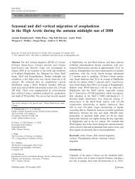
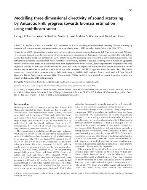
<strong>Modelling</strong> <strong>three</strong>-<strong>dimensional</strong> <strong>directivity</strong> <strong>of</strong> <strong>sound</strong> <strong>scattering</strong><br />
<strong>by</strong> Antarctic krill: progress towards biomass estimation<br />
using multibeam sonar<br />
George R. Cutter, Josiah S. Renfree, Martin J. Cox, Andrew S. Brierley, and David A. Demer<br />
Cutter, G. R., Renfree, J. S., Cox, M. J., Brierley, A. S., and Demer, D. A. 2009. <strong>Modelling</strong> <strong>three</strong>-<strong>dimensional</strong> <strong>directivity</strong> <strong>of</strong> <strong>sound</strong> <strong>scattering</strong> <strong>by</strong><br />
Antarctic krill: progress towards biomass estimation using multibeam sonar. – ICES Journal <strong>of</strong> Marine Science, 66: 1245–1251.<br />
Target strength (TS) estimation is a principal source <strong>of</strong> uncertainty in acoustic surveys <strong>of</strong> Antarctic krill (Euphausia superba). Although<br />
TS is strongly dependent on krill orientation, there is a paucity <strong>of</strong> information in this regard. This paper considers the potential for<br />
narrow-bandwidth, multibeam-echo<strong>sound</strong>er (MBE) data to be used for estimating the orientations <strong>of</strong> krill beneath survey vessels. First,<br />
s<strong>of</strong>tware was developed to predict MBE measurements <strong>of</strong> the <strong>directivity</strong> patterns <strong>of</strong> acoustic <strong>scattering</strong> from individual or aggregated<br />
krill in any orientation. Based on the distorted-wave, Born approximation model (DWBA), <strong>scattering</strong> intensities are predicted vs. MBE<br />
angles for specified distributions <strong>of</strong> krill orientations (pitch, roll, and yaw angles) and swarm densities. Results indicate that certain<br />
distributions <strong>of</strong> orientations, perhaps indicative <strong>of</strong> particular behaviour, should be apparent from the sonar data. The model<br />
results are compared with measurements on krill made using a 200-kHz MBE deployed from a small craft <strong>of</strong>f Cape Shirreff,<br />
Livingston Island, Antarctica, in summer 2006. The stochastic DWBA model is then invoked to explain disparities between the<br />
model predictions and MBE measurements.<br />
Keywords: Antarctic krill, <strong>directivity</strong>, incidence angle, multibeam sonar, orientation, target strength.<br />
Received 11 August 2008; accepted 28 December 2008; advance access publication 18 March 2009.<br />
G. R. Cutter, J. S. Renfree, and D. A. Demer: Southwest Fisheries Science Center, 8604 La Jolla Shores Drive, La Jolla, CA 92037, USA. M. J. Cox and<br />
A. S. Brierley: Gatty Marine Laboratory, School <strong>of</strong> Biology, University <strong>of</strong> St Andrews, Fife KY16 8LB, Scotland, UK. Correspondence to G. R. Cutter:<br />
tel: þ1 858 546 5691; fax: þ1 858 546 5656; e-mail: george.cutter@noaa.gov.<br />
Introduction<br />
High-frequency (70 kHz) acoustic <strong>scattering</strong> from Antarctic krill<br />
(Euphausia superba) is highly directional. For example, the<br />
distorted-wave, Born-approximation model (DWBA; McGehee<br />
et al., 1998) and the Stochastic DWBA model (SDWBA; Demer<br />
and Conti, 2003a; Conti and Demer, 2006) predict that the<br />
target strength (TS) <strong>of</strong> krill at 120 kHz is 20 dB lower for a tilt<br />
angle u ¼ 158 <strong>of</strong>f the dorsal incidence than at u ¼ 08.<br />
Consequently, the TS <strong>of</strong> krill at typical sonar frequencies can<br />
vary substantially, particularly for u , 308.<br />
The orientations <strong>of</strong> in situ krill are variable and largely unknown.<br />
What is known about u for krill was derived from measurements <strong>of</strong><br />
ex situ krill and inferences from data on in situ krill. For krill hovering<br />
in an aquarium, Kils (1981) and Endo (1993) estimated u ¼ 458<br />
(s.d. ¼ 308) andu ¼ 458 (s.d. ¼ 208), respectively. For krill swimming<br />
in a flume, Kils (1981) measured u 5–308, with the<br />
smaller angles corresponding to faster speeds. From acoustic observations,<br />
Chu et al. (1993) estimated u 0–308 for swimming,<br />
encaged krill, whereas Demer and Conti (2005), Conti et al.<br />
(2005), and Conti and Demer (2006) estimated u 11–158<br />
(s.d. ¼ 4–58) for krill beneath a survey vessel. Lawson et al. (2006)<br />
estimated u 108 (s.d. ¼ 608; medianu ¼ –0.58) visually for krill<br />
passing through a towed, video plankton recorder. Most <strong>of</strong> these<br />
observations indicate that krill orientate head-up (positive u)<br />
when at rest and are orientated nearly horizontal (u 08) when<br />
swimming. Consequently, it must be assumed that krill in the wild<br />
can adopt any orientation, depending on their behaviour.<br />
For acoustic surveys <strong>of</strong> krill conducted using a single-beam<br />
echo<strong>sound</strong>er (SBE), u modulates the incidence angle and hence<br />
the measured TS. Measurements <strong>of</strong> volume-back<strong>scattering</strong><br />
strength (S v ¼ TS þ 10 log N, where N is the number <strong>of</strong> scatterers<br />
per cubic metre) are therefore also modulated <strong>by</strong> u. Therefore, the<br />
generally unknown orientation <strong>of</strong> krill is a principal source <strong>of</strong><br />
uncertainty in acoustic estimates <strong>of</strong> their density, abundance,<br />
and biomass. Better knowledge <strong>of</strong> krill orientations, particularly<br />
during acoustic observations, would constitute a major step<br />
towards reducing uncertainty in surveys with SBEs. Perhaps such<br />
information would also allow the use <strong>of</strong> multibeam echo<strong>sound</strong>ers<br />
(MBEs), that have swaths <strong>of</strong> 90–1808, for quantitative surveys <strong>of</strong><br />
krill. At present, the multiple angles <strong>of</strong> incidence associated with<br />
the various beams make quantitative translation <strong>of</strong> echo intensity<br />
to numerical density essentially impossible.<br />
Although some TS models <strong>of</strong> krill are parameterized for any<br />
incidence angle, only variations in TS vs. u have yet been considered<br />
(Martin Traykovski et al., 1998; McGehee et al., 1998;<br />
Demer and Conti, 2003a). Distributions <strong>of</strong> u have been estimated<br />
for krill <strong>by</strong> inverting TS models using broad-bandwidth (Martin<br />
Traykovski et al., 1998) and multifrequency measurements <strong>of</strong> S v<br />
(Chu et al., 1993; Conti et al., 2005; Demer and Conti, 2005;<br />
Conti and Demer, 2006). These methods are ineffective,<br />
# United States Government, National Oceanic and Atmospheric Administration, National Marine Fisheries Service, Southwest Fisheries<br />
Science Center 2009
1246 G. R. Cutter et al.<br />
Figure 1. Three views <strong>of</strong> the shape used to represent a generic krill for the DWBA and SDWBA models; (a) left side, (b) dorsal, and (c) head.<br />
Labels in (a) indicate the dorsal (‘d’) and ventral (‘v’) surfaces, and the head (‘h’) and tail (‘t’) <strong>of</strong> the krill.<br />
however, if the <strong>scattering</strong>-<strong>directivity</strong> pattern (SDP) is complicated<br />
or if the acoustic beam is non-vertical.<br />
Krill can adopt any orientation because <strong>of</strong> natural behaviour,<br />
water motion, or reactions to the presence <strong>of</strong> a survey vessel as<br />
can fish (Gerlotto and Fréon, 1992; Soria et al., 1996; Gerlotto<br />
et al., 2004). The combination <strong>of</strong> krill orientations and the<br />
range <strong>of</strong> beam directions from a wide-swath MBE, or a motionuncompensated<br />
SBE, means that krill could be insonified from<br />
any direction. Therefore, this study considers not only u, but<br />
also any orientation resulting from the pitch, roll, and yaw <strong>of</strong><br />
the krill, combined with variations in the direction <strong>of</strong> the acoustic<br />
beam. Here, the TS values for any incidence angle are modelled<br />
using the DWBA (McGehee et al., 1998), resulting in complete,<br />
<strong>three</strong>-<strong>dimensional</strong>, frequency-specific, SDPs for krill, similar to<br />
those produced for fish <strong>by</strong> Jech and Horne (2002) and Towler<br />
et al. (2003). Using the krill SDPs, and a simulation model <strong>of</strong><br />
Table 1. Values <strong>of</strong> cylinder radii a used for the krill-shape model.<br />
a McGehee (m) a fat (m) x (m) y (m) z (m)<br />
0.000 0.000 3.835 10 22 0.000 0.000<br />
2.147 10 24 3.006 10 24 3.686 10 22 0.000 9.149 10 24<br />
6.525 10 24 9.136 10 24 3.405 10– 2 0.000 1.792 10 23<br />
1.130 10 23 1.581 10 23 2.942 10 22 0.000 2.455 10 23<br />
1.354 10 23 1.895 10 23 2.662 10 22 0.000 2.437 10 23<br />
1.447 10 23 2.026 10 23 2.353 10 22 0.000 2.455 10 23<br />
1.596 10 23 2.235 10 23 2.070 10 22 0.000 2.306 10 23<br />
1.550 10 23 2.170 10 23 1.770 10 22 0.000 2.250 10 23<br />
1.652 10 23 2.313 10 23 1.519 10 22 0.000 2.054 10 23<br />
1.904 10 23 2.666 10 23 1.285 10 22 0.000 1.848 10 23<br />
1.755 10 23 2.457 10 23 1.053 10 22 0.000 1.690 10 23<br />
1.652 10 23 2.313 10 23 8.467 10 23 0.000 1.690 10 23<br />
1.382 10 23 1.934 10 23 6.647 10 23 0.000 2.063 10 23<br />
1.102 10 23 1.542 10 23 2.969 10 23 0.000 2.474 10 23<br />
5.508 10 24 7.711 10 24 0.000 0.000 3.557 10 23<br />
The density contrast was g ¼ 1.0357, and the <strong>sound</strong>-speed contrast h ¼<br />
1.0279. The number <strong>of</strong> cylinders, N bcyl , was 6, 10, 15, and 25 at frequencies<br />
38, 70, 120, and 200 kHz, respectively.<br />
the MBE developed <strong>by</strong> Cutter and Demer (2007), distributions<br />
<strong>of</strong> <strong>scattering</strong> intensity are predicted for many beam directions<br />
and various distributions <strong>of</strong> krill orientations and aggregation<br />
densities. These simulation results are compared with MBE data.<br />
Although the work focuses on krill, the findings here are also relevant<br />
to surveys <strong>of</strong> any pelagic species conducted with MBEs and<br />
SBEs.<br />
Methods<br />
<strong>Modelling</strong> krill shape<br />
The DWBA was parameterized with a generic krill shape<br />
(Figure 1) comprising multiple, contiguous cylinders distributed<br />
along a curve (McGehee et al., 1998). Shape parameters include<br />
the cylinder radii a (m), the density contrast g, the <strong>sound</strong>-speed<br />
contrast h, and the locations <strong>of</strong> the centres <strong>of</strong> each cylinder r, in<br />
rectangular coordinates (Table 1). As in Demer and Conti<br />
(2003b, 2005) and Conti and Demer (2006), the radii (a) were<br />
40% larger than those <strong>of</strong> the starved krill modelled in McGehee<br />
Figure 2. Definitions <strong>of</strong> pitch, roll, and yaw used in the simulations.<br />
A horizontal krill with the dorsal side upwards has zero pitch.<br />
Positive pitch corresponds to head-up rotations.
<strong>Modelling</strong> krill <strong>three</strong>-<strong>dimensional</strong> <strong>scattering</strong> density 1247<br />
et al. (1998). The standard krill length, L ¼ 38.35 mm, is from<br />
the front <strong>of</strong> the eyes to the tip <strong>of</strong> the telson. The number <strong>of</strong> cylinders,<br />
N bcyl , varied with the acoustic frequency, as in Conti and<br />
Demer (2006).<br />
<strong>Modelling</strong> SDPs<br />
The DWBA was used to model krill SDPs for the commonly<br />
employed acoustic frequencies <strong>of</strong> 38, 70, 120, and 200 kHz.<br />
Following the reference frame and angle definitions in McGehee<br />
et al. (1998), the krill shapes were transformed, first <strong>by</strong> translating<br />
the central axis <strong>of</strong> the krill to the x-axis, then rotating the<br />
krill about that axis over 3608 at 18 intervals. For each roll-angle<br />
interval, the model predicted TS for 18 intervals over 3608 in the<br />
vertical plane. Therefore, TS data were modelled for all directions,<br />
and the results at each interval were combined to form the<br />
complete SDP.<br />
SDPs were similarly generated for 120 and 200 kHz using the<br />
SDWBA. TS values were estimated for ten realizations with<br />
random phases and s.d. (f) ¼ 0.7070 radians; see Demer and<br />
Conti (2003a, b) for details.<br />
<strong>Modelling</strong> multibeam measurements<br />
The 200-kHz SDPs calculated with both the DWBA and SDWBA<br />
were used in a simulation program (Cutter and Demer, 2007) to<br />
predict MBE measurements <strong>of</strong> <strong>scattering</strong> intensity from krill<br />
aggregations with specified densities (number per m 3 per beam)<br />
and orientation distributions, defined <strong>by</strong> the mean + s.d. for<br />
normal angle distributions and the minima and maxima for<br />
uniform distributions. Krill orientations were controlled <strong>by</strong> <strong>three</strong><br />
angles. The pitch describes rotation about the lateral axis <strong>of</strong> the<br />
krill, or head-up, tail-down motion; the roll describes rotation<br />
about the head–tail axis; and the yaw describes rotation about<br />
the vertical axis (Figure 2). In each simulation, the number <strong>of</strong><br />
krill was varied from 25 to 50 per m 3 . These densities were large<br />
enough to produce distributions with approximately normal<br />
pitch and uniform yaw. The same distributions <strong>of</strong> krill orientation<br />
were used for all beams. It was assumed that each krill was insonified<br />
on the beam axis, where the acoustic sensitivity is at a<br />
maximum. Outputs <strong>of</strong> the simulation included TS for each<br />
beam and each krill, and the mean and distribution <strong>of</strong> S v , normalized<br />
to one animal per unit volume for the krill insonified <strong>by</strong> each<br />
beam. Hence, the model results can be adjusted to predict S v for<br />
any number (N) <strong>of</strong> krill as the sum <strong>of</strong> the normalized S v and<br />
10 log(N). Data were simulated for a subset (at intervals <strong>of</strong> 108)<br />
<strong>of</strong> beams spanning an athwartships swath <strong>of</strong> 1808 (+908 to each<br />
side <strong>of</strong> the vertical).<br />
Multibeam data<br />
A 200-kHz MBE (Kongsberg-Mesotech SM2000/SM20) was used<br />
to survey krill in shallow water (,200 m) <strong>of</strong>f Cape Shirreff,<br />
Livingston Island, Antarctica (Cox et al., in press) from 2 to 9<br />
February 2006. The MBE was deployed from a small (6 m long)<br />
inflatable boat (Mark V Zodiac). The MBE has 128 beams spanning<br />
a 1208 swath. The transmit power was ‘medium’, pulse duration<br />
was 825 ms, maximum range was 200 m, TVG was<br />
20 log R þ 2 aR (where R is the range and a the absorption coefficient).<br />
The raw data were recorded and gain compensation was<br />
applied during post-processing.<br />
The S v measurements from the MBE were calibrated (<strong>of</strong>fset ¼<br />
–71.2 dB) against measurements made concurrently with a<br />
Figure 3. SDPs representing the TS (dB) for any beam-incidence<br />
angle about a krill (E. superba); results from the DWBA model for (a)<br />
38 kHz, (b) 70 kHz, (c) 120 kHz, (d) 200 kHz, and (e) the krill shape<br />
depicted within the 120 kHz SDP illustrating the incidence<br />
directions.<br />
calibrated 200-kHz SBE (Simrad ES60; see Cox et al., in press,<br />
for details). The S v from krill swarms were exported from<br />
Echoview (Myriax, Hobart, Australia) for calculations <strong>of</strong> the<br />
mean and s.d. <strong>of</strong> S v vs. beam direction as in Cutter and Demer<br />
(2007). These data were compared with patterns predicted <strong>by</strong><br />
the simulation. Additionally, S v vs. range and bearing were<br />
exported for all swarms identified using Echoview’s schooldetection<br />
routine in the multibeam module (Cox et al., in<br />
press). A random set <strong>of</strong> 100 pings from these data was examined<br />
for patterns <strong>of</strong> S v vs. beam direction.
1248 G. R. Cutter et al.<br />
Figure 5. TS predicted <strong>by</strong> the multibeam-<strong>directivity</strong> model for<br />
200 kHz, beam directions from –908 to 908, and krill-pitch angles <strong>of</strong><br />
(a) 08, (b) 58, (c) 108, (d) 208, and (e) 308.<br />
Figure 4. SDPs representing the TS (dB) for any beam-incidence<br />
angle about a krill (E. superba), resulting from the SDWBA model for<br />
(a) 120 kHz, and (b) 200 kHz.<br />
Results<br />
Krill SDPs<br />
SDPs based on the DWBA at 38, 70, 120, and 200 kHz were imaged<br />
<strong>three</strong>-<strong>dimensional</strong>ly (Figure 3). The complexity and <strong>directivity</strong><br />
increase with frequency. At 38 kHz, the SDP resembles a simple<br />
disc or compressed sphere, with a nearly circular main lobe<br />
(TS – 80 dB) in the plane defined <strong>by</strong> the lateral (y) and<br />
dorso-ventral (z) axes (Figure 3a). The SDPs at 70 and 120 kHz<br />
have a narrow main lobe and two (70 kHz; Figure 3b) to four<br />
(120 kHz; Figure 3c) side lobes, tilted in the y–z plane towards<br />
the head–tail axis. The SDP for 200 kHz has a very narrow main<br />
lobe and several narrow side lobes in close proximity to dorsal<br />
incidence, with peaks nearly equal to the main lobe (Figure 3d).<br />
Among these frequencies, krill TS was highest at 120 kHz with a<br />
peak value <strong>of</strong> 265.4 dB at dorsal incidence.<br />
For comparison, the SDPs based on the SDWBA at 120 and<br />
200 kHz are presented in Figure 4. The phase variations modelled<br />
in the SDWBA had little effect on the dorso-ventral <strong>scattering</strong>.<br />
However, the SDWBA predicted an increase in the TS observed<br />
from the head and tail directions and reduced <strong>directivity</strong> <strong>of</strong>f the<br />
main lobes. These effects were most pronounced in the 120-kHz<br />
SDP, where the <strong>scattering</strong> was nearly uniform for all incidence<br />
angles away from the primary lobe, and include a more subtle,<br />
tilted secondary lobe.<br />
Modelled multibeam measurements<br />
The 200-kHz SDP from the DWBA was used to simulate measurements<br />
<strong>of</strong> S v vs. beam direction for an MBE with 1808 swath.<br />
The resulting S v vs. pitch is displayed in Figure 5. When krill are<br />
horizontal and aligned with the ship, the MBE beams intersect<br />
the main lobe <strong>of</strong> the SDP at all incidence angles, resulting in a<br />
nearly constant TS <strong>of</strong> approximately 270 dB. If pitch ¼ 58, the<br />
S v observed in the vertical beam changed <strong>by</strong> 25 dB; and <strong>by</strong><br />
nearly 210 dB in the beams 308 to either side <strong>of</strong> the vertical.<br />
To simulate MBE measurements <strong>of</strong> S v at 200 kHz from a krill<br />
aggregation with a pitch distribution N(118, 48), as described <strong>by</strong><br />
Conti and Demer (2006), and a uniform distribution <strong>of</strong> yaw,<br />
DWBA-SDPs representing 25 krill were insonified <strong>by</strong> each beam.<br />
The resulting mean S v were 5–10 dB higher in the beams +208<br />
from the vertical compared with the outer beams. When the simulated<br />
pitch distribution was broader [e.g. N(118, 248)], the values<br />
<strong>of</strong> S v were nearly equivalent, with approximately equal variance vs.<br />
beam direction (Figure 6).<br />
Multibeam survey data<br />
Various patterns <strong>of</strong> S v vs. beam direction were apparent in the MBE<br />
data, but none was dominant. The observed patterns included nearly<br />
uniform, trending, alternating high and low, and occasionally an
<strong>Modelling</strong> krill <strong>three</strong>-<strong>dimensional</strong> <strong>scattering</strong> density 1249<br />
Figure 6. Target-strength distributions predicted <strong>by</strong> the multibeam<strong>directivity</strong><br />
model for 200 kHz and 25 krill per beam. The krill are<br />
orientated with uniform yaw and (a) pitchN(118, 48), and (b)<br />
pitchN(118, 248). The realized distributions <strong>of</strong> yaw were<br />
(a) U(–1458, 1408), and (b) U(–898, 828).<br />
absence <strong>of</strong> krill in the beams at and near vertical incidence<br />
(Figure 7). The S v vs. beam direction was variable, with S v ranging<br />
+2–10 dB from the mean value <strong>of</strong> each pattern (Figure 7).<br />
Trends and patterns <strong>of</strong> S v vs. beam direction were evident in some<br />
pings, but none could be clearly matched to the simulation<br />
results. For example, the simulation predicted that for a mean<br />
pitch ¼ 118, S v should be 5 dB lower for the vertical vs. outer<br />
beams when yaw ¼ 08, and higher in the near-vertical beams for<br />
non-zero, variable yaw. Lower S v in near-vertical beams was apparent<br />
in at least one case, but this could not be attributed uniquely to<br />
yaw. The result could also have been caused <strong>by</strong> non-uniform krill<br />
density that could occur naturally or a reaction to the vessel.<br />
Discussion<br />
When surveying krill with an SBE at the common frequencies <strong>of</strong><br />
70, 120, and 200 kHz, TS and S v are highly sensitive to small<br />
changes in pitch, but roll has negligible effect. However, when surveying<br />
with a high-frequency MBE, the pitch, roll, and yaw <strong>of</strong> krill<br />
are all important, because the SDPs are complex and the large<br />
swath insonifies the krill at many incidence angles.<br />
For SBEs without motion compensation, the vessel’s roll<br />
and pitch will result in non-vertical beams. The SDPs for krill at<br />
70–200 kHz are most variable within +458 <strong>of</strong> dorsal-aspect<br />
incidence. Within a narrow range <strong>of</strong> beam directions (+158),<br />
TS <strong>of</strong> krill can vary <strong>by</strong> 10 dB (at 200 kHz), depending on the<br />
krill orientations. If a krill yaws a mere 158 <strong>of</strong>f the vessel-track<br />
direction, and the beam direction varies from 08 to 158 because<br />
<strong>of</strong> vessel motion (for the SBE), or for that portion <strong>of</strong> an MBE<br />
swath, the measured TS can range from 270.4 to 281.7 dB.<br />
Therefore, krill yaw is important even for surveys with SBEs,<br />
particularly at frequencies .120 kHz.<br />
The krill TS and the SDP depend on the animal size relative to<br />
the <strong>sound</strong> wavelength. The krill model used in this study was<br />
chosen to be consistent with the size <strong>of</strong> krill modelled in previous<br />
studies (McGehee et al., 1988; Demer and Conti, 2003b). Demer<br />
and Conti (2003b) measured krill length-frequency distributions<br />
from 20 to 50 mm, with an overall mean <strong>of</strong> 31.6 mm (s.d. ¼<br />
6.6 mm). Larger krill would probably have slightly higher mean<br />
TS values and somewhat more complicated SDPs at lower frequencies<br />
(,200 kHz). Similarly, the SDP <strong>of</strong> smaller krill at 200 kHz<br />
would probably have a simpler geometry, a lower <strong>directivity</strong>, and<br />
a lower mean TS averaged over all angles.<br />
For krill orientated with pitchN(118, 48) (Conti and Demer,<br />
2006) and yawU(21498, 1398), the simulations based on the<br />
SDWBA at 200 kHz indicate an obvious pattern in the multibeam<br />
data (Figure 8). Specifically, measured <strong>scattering</strong> intensities should<br />
be nearly 8 dB higher for the near-vertical beams relative to the<br />
outer beams. This was not observed in the field data.<br />
Many explanations are possible for the absence <strong>of</strong> the expected<br />
patterns in the MBE field data. For example, the pitch distribution<br />
might not be the N(118,48) estimated <strong>by</strong> Conti and Demer (2006)<br />
for krill beneath a large vessel surveying at speed, or the krill might<br />
have been dispersed throughout each beam, as opposed to being<br />
only on the beam axes. That is, the MBE measurements were convolved<br />
with the beam patterns <strong>of</strong> each beam. A refinement <strong>of</strong> the<br />
simulation model should therefore account for beam-pattern<br />
effects. Alternatively, measurements with a fully calibrated MBE,<br />
particularly a split-beam instrument such as the Simrad ME70,<br />
could be deconvolved with the known beam patterns before<br />
comparison with the simulation results. Another hypothesis is<br />
that the krill changed their natural orientations or locations in<br />
vessel-avoidance reactions, as suggested <strong>by</strong> the swarms detected<br />
in the outer beams compared with those in the inner beams<br />
(Figure 7).<br />
Non-uniform orientation distributions are difficult to estimate<br />
even for scatterers with high and known SDPs. Hence, the estimation<br />
<strong>of</strong> scatterers’ orientation from narrowband MBE data<br />
requires restrictive conditions. However, concurrent multibeam<br />
and multifrequency split-beam measurement spanning 38–200 kHz<br />
could better constrain the problem and provide better estimates<br />
<strong>of</strong> scatterer’ orientations.<br />
Conclusions<br />
If the orientation angles <strong>of</strong> the insonified krill are not known, the<br />
measured TS and S v include large uncertainties. A calibrated MBE<br />
is not prerequisite to detect the S v vs. beam-direction patterns<br />
associated with known consistent distributions <strong>of</strong> krill orientations.<br />
Therefore, krill orientations can be estimated from narrowband,<br />
multibeam data if all krill in an aggregation are<br />
orientated similarly across all beam directions, for example if<br />
krill are responding to a vessel in a predictable manner.<br />
However, the MBE must be calibrated to allow a quantitative comparison<br />
with a calibrated, split-beam SBE.
1250 G. R. Cutter et al.<br />
Figure 7. Measured S v vs. beam direction from the 200 kHz MBE deployed in Antarctica. Examples <strong>of</strong> various patterns: (a) nearly uniform, (b)<br />
trending, (c) variable, (d) variable with diminished near-vertical incidence; in (e) and (f) there are no krill in the central, near-vertical beams.<br />
The complexities <strong>of</strong> high-frequency SDPs make it difficult to<br />
estimate krill-pitch distributions from measurements with a<br />
single-frequency MBE. In fact, the MBE measurements <strong>of</strong> S v vs.<br />
beam direction in this study did not conform consistently to any<br />
<strong>of</strong> the simulation predictions. The simulations may be improved<br />
<strong>by</strong> accounting for additional factors, such as krill-length distributions<br />
and variations in their orientations within a swarm. In<br />
addition, the beam pattern, <strong>of</strong> the MBE should be taken into<br />
account. Either the simulated S v should be convolved with the<br />
expected beam patterns, or the measured S v should be deconvolved<br />
with the calibrated beam patterns. Future studies should<br />
include independent observations <strong>of</strong> krill orientation during<br />
acoustic surveys, perhaps using visual techniques.<br />
Figure 8. S v vs. beam direction predicted <strong>by</strong> the SDWBA model for<br />
200 kHz. Results for 25 krill per beam with pitchN(118, 48) and<br />
yawU(–1498, 1398).<br />
Acknowledgements<br />
We are grateful to Derek Needham and Mike Patterson (Sea<br />
Technology Services) for developing the MBE transducerdeployment<br />
apparatus, Steve Sessions (SWFSC) for adeptly<br />
driving the Zodiac inflatable boat in the <strong>of</strong>ten harsh conditions
<strong>Modelling</strong> krill <strong>three</strong>-<strong>dimensional</strong> <strong>scattering</strong> density 1251<br />
<strong>of</strong> the Southern Ocean, and the UK National Environmental<br />
Research Council, Royal Society, and the US Antarctic Marine<br />
Living Resources Program for co-sponsoring the data-collection<br />
portion <strong>of</strong> this investigation. We thank Jeff Condiotty <strong>of</strong> Simrad,<br />
USA, for the use <strong>of</strong> the SM2000.<br />
References<br />
Chu, D., Foote, K. G., and Stanton, T. K. 1993. Further analysis <strong>of</strong><br />
target-strength measurements <strong>of</strong> Antarctic krill at 38 and 120<br />
kHz: comparison with deformed-cylinder model and inference <strong>of</strong><br />
orientation distribution. Journal <strong>of</strong> the Acoustical Society <strong>of</strong><br />
America, 93: 2985–2988.<br />
Conti, S. G., and Demer, D. A. 2006. Improved parameterization <strong>of</strong> the<br />
SDWBA for estimating krill target strength. ICES Journal <strong>of</strong><br />
Marine Science, 63: 928–935.<br />
Conti, S. G., Demer, D. A., and Brierley, A. S. 2005. Broad-bandwidth,<br />
<strong>sound</strong> <strong>scattering</strong>, and absorption from krill (Meganyctiphanes norvegica),<br />
mysids (Praunus flexuosus and Neomysis integer), and<br />
shrimp (Crangon crangon). ICES Journal <strong>of</strong> Marine Science, 62:<br />
956–965.<br />
Cox, M. J., Demer, D. A., Warren, J. D., Cutter, G. R., and Brierley,<br />
A. S. Multibeam echo<strong>sound</strong>er observations <strong>of</strong> Antarctic krill<br />
(Euphausia superba) swarms and interactions between krill and<br />
air breathing predators. Deep Sea Research II, in press.<br />
Cutter, G. R., and Demer, D. A. 2007. Accounting for <strong>scattering</strong> <strong>directivity</strong><br />
and fish behaviour in multibeam-echo<strong>sound</strong>er surveys. ICES<br />
Journal <strong>of</strong> Marine Science, 64: 1664–1674.<br />
Demer, D. A., and Conti, S. G. 2003a. Reconciling theoretical versus<br />
empirical target strengths <strong>of</strong> krill: effects <strong>of</strong> phase variability on<br />
the distorted-wave Born approximation. ICES Journal <strong>of</strong> Marine<br />
Science, 60: 429–434.<br />
Demer, D. A., and Conti, S. G. 2003b. Validation <strong>of</strong> the stochastic<br />
distorted-wave Born approximation model with broad bandwidth<br />
total target strength measurements <strong>of</strong> Antarctic krill. ICES Journal<br />
<strong>of</strong> Marine Science, 60: 625–635.<br />
Demer, A. D., and Conti, S. G. 2005. New target-strength model indicates<br />
more krill in the Southern Ocean. ICES Journal <strong>of</strong> Marine<br />
Science, 62: 25–32.<br />
Endo, Y. 1993. Orientation <strong>of</strong> Antarctic krill in an aquarium. Nippon<br />
Suisan Gakkaishi, 59: 465–468.<br />
Gerlotto, F., Castillo, J., Saavedra, A., Barbieri, M. A., Espejo, M., and<br />
Cotel, P. 2004. Three-<strong>dimensional</strong> structure and avoidance behaviour<br />
<strong>of</strong> anchovy and common sardine schools in central, southern<br />
Chile. ICES Journal <strong>of</strong> Marine Science, 61: 1120–1126.<br />
Gerlotto, F., and Fréon, P. 1992. Some elements on vertical avoidance<br />
<strong>of</strong> fish schools to a vessel during acoustic surveys. Fisheries<br />
Research, 14: 251–259.<br />
Jech, J. M., and Horne, J. K. 2002. Three-<strong>dimensional</strong> visualization <strong>of</strong><br />
fish morphometry and acoustic backscatter. Acoustic Research<br />
Letters Online, 3(1): 35–40.<br />
Kils, U. 1981. The swimming behaviour, swimming performance and<br />
energy balance <strong>of</strong> Antarctic krill Euphausia superba. BIOMASS<br />
Scientific Series, 3. 122 pp.<br />
Lawson, G. L., Wiebe, P. H., Ashjian, C. J., Chu, D., and Stanton, T. K.<br />
2006. Improved parameterization <strong>of</strong> Antarctic krill target-strength<br />
models. Journal <strong>of</strong> the Acoustical Society <strong>of</strong> America, 119:<br />
232–242.<br />
Martin Traykovski, L. V., O’Driscoll, R. L., and McGehee, D. E. 1998.<br />
Effect <strong>of</strong> orientation on broadband acoustic <strong>scattering</strong> <strong>of</strong> Antarctic<br />
krill Euphausia superba: implications for inverting zooplankton<br />
spectral acoustic signatures for angle <strong>of</strong> orientation. Journal <strong>of</strong><br />
the Acoustical Society <strong>of</strong> America, 104: 2121–2135.<br />
McGehee, D. E., O’Driscoll, R. L., and Martin Traykovski, L. V. 1998.<br />
Effects <strong>of</strong> orientation on acoustic <strong>scattering</strong> from Antarctic krill at<br />
120 kHz. Deep Sea Research II, 45: 1273–1294.<br />
Soria, M., Fréon, P., and Gerlotto, F. 1996. Analysis <strong>of</strong> vessel influence<br />
on spatial behaviour <strong>of</strong> fish schools using a multibeam sonar and<br />
consequences for biomass estimates <strong>by</strong> echo<strong>sound</strong>er. ICES<br />
Journal <strong>of</strong> Marine Science, 53: 453–458.<br />
Towler, R. H., Jech, J. M., and Horne, J. K. 2003. Visualizing fish movement,<br />
behaviour, and acoustic backscatter. Aquatic Living<br />
Resources, 16: 277–282.<br />
doi:10.1093/icesjms/fsp040