Nanoporous Gold Electrocatalysis for Ethylene Monitoring ... - CID, Inc.
Nanoporous Gold Electrocatalysis for Ethylene Monitoring ... - CID, Inc.
Nanoporous Gold Electrocatalysis for Ethylene Monitoring ... - CID, Inc.

You also want an ePaper? Increase the reach of your titles
YUMPU automatically turns print PDFs into web optimized ePapers that Google loves.
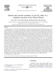
174 Shekarriz and L. Allen: <strong>Nanoporous</strong> <strong>Gold</strong> <strong>Electrocatalysis</strong> <strong>for</strong> <strong>Ethylene</strong> <strong>Monitoring</strong><br />
Fig. 4. Scanning electron<br />
microscope (SEM) images<br />
of nanoporous gold used<br />
as an electrocatalyst in the<br />
current sensing approach.<br />
The two images are at<br />
magnifications of 20,000x<br />
(left) and 100,000x (right)<br />
revealing features smaller<br />
than 10 nm.<br />
Relative Sensitivity<br />
1<br />
0.8<br />
0.6<br />
0.4<br />
0.2<br />
Response, µA<br />
140<br />
120<br />
100<br />
80<br />
60<br />
40<br />
Raw Data<br />
Corrected Data<br />
Linear (Raw Data)<br />
Linear (Corrected Data)<br />
y = 12.283x + 3.4<br />
R 2 = 0.9998<br />
0<br />
0.00 0.20 0.40 0.60 0.80 1.00<br />
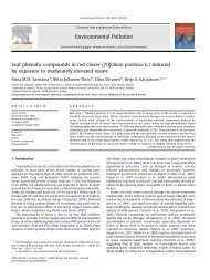
Fig. 5. Sensitivity or sensor response versus apparent surface<br />
area of catalyst.<br />
In general, the relationship between the surface area of<br />
the catalyst and the sensitivity or sensor response followed<br />
a monotonic relationship as shown in Fig. 5.<br />
Standard Gas Measurements<br />
A critical characteristic of a sensing device is whether or<br />
not it responds linearly over the desired operating range.<br />
Nonlinear response demands multiple-point calibration<br />
and the number of points required is a function of degree<br />
of departure from linearity. As shown in Fig. 6, the current<br />
electrocatalytic cell provides extremely linear response<br />
revealed by the trendline equations, extending to<br />
concentrations well above 100 ppm. The two graphs<br />
shown represent the raw data and the corrected data.<br />
Correction only removes the background leakage current,<br />
which shows up as a bias current in the data. Note<br />
that this particular electrocatalyst showed a response of<br />
12.179 µA ppm –1 . Using the linearity property of our<br />
electrocatalytic sensor, which is typical of first order catalytic<br />
reactions, only two points are required <strong>for</strong> calibration<br />
of the device, zero and the maximum expected concentration,<br />
say 100 ppm. For better accuracy, the maximum<br />
point <strong>for</strong> calibration is selected to match the expected<br />
range of measurements, say 1 ppm <strong>for</strong> 0 to 1 ppm<br />
measurements.<br />
Reaction Rate<br />
Normalized Surface Area<br />
20<br />
y = 12.179x<br />
R 2 = 0.9998<br />
0<br />
0.01 0.1 1 1 0<br />
Fig. 6. Sensor linearity at low ethylene concentrations of below<br />
10 ppm. The linear curves on a logarithmic scale provide<br />
an expanded view of small concentrations while they have<br />
exponential manifestations as shown above.<br />
Efficient electrocatalytic reaction is a critical part of the<br />
sensor. Fig. 7 shows two consecutive injections of ethylene<br />
directly into the device (see Fig. 3) such that the concentration<br />
was raised to approximately 100 ppb <strong>for</strong> each<br />
trial. By recirculating air over the electrocatalyst, the concentration<br />
of ethylene was allowed to drop through electrocatalytic<br />
decomposition. In this particular experiment,<br />
the consecutive data points were collected every 3 s, and<br />
each trial took roughly 4 min to bring the ethylene concentration<br />
to near zero. The 1/e characteristic time constant<br />
or the time it took <strong>for</strong> ethylene concentration to<br />
drop below 40 ppb was in average 1 min. Note that once<br />
a sample was injected into the device, it took between 5<br />
and 10 s <strong>for</strong> the maximum concentration to be realized.<br />
The insert in this plot shows a magnified region of the<br />
data over a 1 min period, where the pulse-to-pulse signal<br />
fluctuation is ±5 ppb, but the 10 s average shows lower<br />
fluctuation in the results. Clearly, <strong>for</strong> very rapidly changing<br />
signal, <strong>for</strong> example near the peak shown in Fig. 7,<br />
time averaging will truncate the data. However, most real<br />
systems in postharvest applications will not undergo rapid<br />
changes in concentration and averages over 1 min<br />
should be more than adequate <strong>for</strong> signal processing and<br />
data interpretation.<br />
When sampling the air in a closed system, both ethylene<br />
generation and destruction may be taking place simultaneously,<br />
and the total ethylene present in the system<br />
will vary according to the following equation:<br />
∀ e,s<br />
∫<br />
t<br />
= [ ∀·<br />
g,s<br />
( t’ ) – ∀·<br />
d,s ( t’ )]dt’<br />
( 1)<br />
o<br />
Concentration, ppm<br />
Europ.J.Hort.Sci. 4/2008