InfraCal TOG/TPH Analyzer - Wilks Enterprise, Inc.
InfraCal TOG/TPH Analyzer - Wilks Enterprise, Inc.
InfraCal TOG/TPH Analyzer - Wilks Enterprise, Inc.

Create successful ePaper yourself
Turn your PDF publications into a flip-book with our unique Google optimized e-Paper software.
<strong>Wilks</strong> <strong>Enterprise</strong>, <strong>Inc</strong>.<br />
140 Water Street · South Norwalk, CT 06854<br />
203 855 9136 · 203 838 9868<br />
www.wilksIR.com · info@wilksir.com<br />
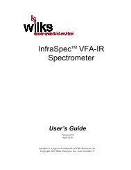
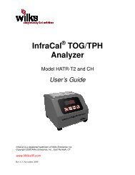
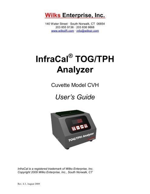
<strong>InfraCal</strong> ® <strong>TOG</strong>/<strong>TPH</strong><br />
<strong>Analyzer</strong><br />
Cuvette Model CVH<br />
User’s Guide<br />
<strong>InfraCal</strong> is a registered trademark of <strong>Wilks</strong> <strong>Enterprise</strong>, <strong>Inc</strong>.<br />
Copyright 2009 <strong>Wilks</strong> <strong>Enterprise</strong>, <strong>Inc</strong>., South Norwalk, CT<br />
Rev. 4.3, August 2009
Table of Contents<br />
1. <strong>InfraCal</strong> <strong>TOG</strong>/<strong>TPH</strong> <strong>Analyzer</strong>, Model CVH Overview ..................................................... 4<br />
1.1. Introduction ..........................................................................................................................4<br />
1.2. Basic measurement concept ..................................................................................................4<br />
1.3. <strong>Analyzer</strong> description .............................................................................................................4<br />
1.3.1. Front operating panel .....................................................................................................4<br />
1.3.2. Back panel .....................................................................................................................5<br />
1.3.3. Description of the push button controls ..........................................................................6<br />
1.4. <strong>Analyzer</strong> Features .................................................................................................................6<br />
1.4.1. Internal Calibration: ......................................................................................................6<br />
1.4.2. External Communication: ..............................................................................................6<br />
1.4.3. Recall Function/Averaging Results ................................................................................6<br />
1.4.4. Printing the Result .........................................................................................................6<br />
2. Getting Started .............................................................................................................. 7<br />
2.1. Installation ...........................................................................................................................7<br />
2.1.1. Location.........................................................................................................................7<br />
2.1.2. Power Requirements ......................................................................................................7<br />
2.1.3. Warm up time ................................................................................................................7<br />
2.2. Zeroing the <strong>Analyzer</strong> ............................................................................................................7<br />
2.2.1. Establishing Zero ...........................................................................................................7<br />
2.2.2. Zero Check ....................................................................................................................8<br />
3. <strong>Analyzer</strong> Calibration ..................................................................................................... 8<br />
3.1. Data Presentation..................................................................................................................8<br />
3.2. Considerations for Calibration Standards ..............................................................................8<br />
3.2.1. Calibration correlated to an Alternate Method................................................................8<br />
3.3. Preparing Calibration Standards ...........................................................................................9<br />
3.3.1. Preparing Volumetric Standards ....................................................................................9<br />
3.3.2. Preparing Gravimetric Standards ................................................................................. 10<br />
3.4. Calibrating in the <strong>Analyzer</strong>................................................................................................. 11<br />
3.4.1. Selecting the Calibration Mode .................................................................................... 11<br />
3.4.2. Setting the evaporation timer ....................................................................................... 11<br />
Timer Programming................................................................................................................... 11<br />
3.4.3. Collecting calibration data ........................................................................................... 12<br />
3.4.4. Entering the User Calibration Data with the Edit program ........................................... 12<br />
3.4.5. User Calibration Mode Procedure: ............................................................................... 13<br />
3.4.6. Calibration printing ..................................................................................................... 13<br />
4. Analyzing an Oil Sample ............................................................................................ 13<br />
4.1. <strong>Analyzer</strong> Pre-Check ............................................................................................................ 13<br />
4.2. 10 to 1 Extraction Procedure for Oil in Water ..................................................................... 13<br />
4.2.1. Supplies Needed for Extraction in Water...................................................................... 13<br />
4.2.2. Considerations: ............................................................................................................ 14<br />
4.2.3. Total Oil and Grease (<strong>TOG</strong>) Extraction from Water ..................................................... 14<br />
4.2.4. Total Petroleum Hydrocarbon (<strong>TPH</strong>) Extraction from Water ........................................ 15<br />
4.3. 1 to 1 Extraction Procedure for Oil in Soil .......................................................................... 15<br />
4.3.1. Supplies Needed .......................................................................................................... 15<br />
4.3.2. Total Oil and Grease (<strong>TOG</strong>) Extraction from Soil ........................................................ 15<br />
4.3.3. Total Petroleum Hydrocarbon (<strong>TPH</strong>) Extraction from Soil ........................................... 16<br />
2
4.4. Dilution Procedures ............................................................................................................ 16<br />
4.4.1. 10:1 Dilution ............................................................................................................... 16<br />
4.5. Averaged Results Display ................................................................................................... 16<br />
5. Detailed Sample Stage Description ........................................................................... 17<br />
5.1. Cuvette (CVH) sample stage ............................................................................................... 17<br />
5.1.1. Cuvette Sample Stage Description................................................................................ 17<br />
5.1.2. Cuvette (Model CVH) Measurement Concept............................................................... 18<br />
5.1.3. Cuvette Considerations ................................................................................................ 18<br />
6. <strong>Analyzer</strong> Specifications .............................................................................................. 19<br />
6.1. External Power Requirements: ............................................................................................ 19<br />
6.2. Physical: ............................................................................................................................. 19<br />
6.3. Environmental: ................................................................................................................... 19<br />
6.4. Electrical ............................................................................................................................ 19<br />
6.5. Calibration: ........................................................................................................................ 20<br />
7. <strong>Analyzer</strong> Communications Interface .......................................................................... 20<br />
7.1. Abstract .............................................................................................................................. 20<br />
7.2. Physical Connection ........................................................................................................... 20<br />
7.3. Communications port setup parameters............................................................................... 21<br />
7.4. Operation ........................................................................................................................... 21<br />
7.5. Data Logging ...................................................................................................................... 21<br />
7.6. Remote Zero Balance Control ............................................................................................. 22<br />
7.7. Remote Calibration Control ................................................................................................ 22<br />
8. Service and Customer Support .................................................................................. 23<br />
Appendix A: Alternate Data Presentation ............................................................................... 24<br />
Appendix B-Correlation to an Alternate method..................................................................... 25<br />
Appendix C: Solvent Options ................................................................................................. 26<br />
List of Figures<br />
Figure 1 - The <strong>InfraCal</strong> <strong>TOG</strong>/<strong>TPH</strong> <strong>Analyzer</strong>: Front View of <strong>Analyzer</strong> .................................... 4<br />
Figure 2: The Display and Control Panel .................................................................................. 5<br />
Figure 3: The <strong>TOG</strong>/<strong>TPH</strong> <strong>Analyzer</strong>: Rear View ........................................................................ 5<br />
Figure 4: The <strong>TOG</strong>/<strong>TPH</strong> <strong>Analyzer</strong> Model CVH Sample Stage: Front View .......................... 17<br />
Figure 5: The <strong>TOG</strong>/<strong>TPH</strong> <strong>Analyzer</strong> Model CVH: Top View ................................................... 17<br />
Figure 6: Measurement of IR Absorption with a Cuvette ....................................................... 18<br />
3
_________________________________________________________________________<br />
1. <strong>InfraCal</strong> <strong>TOG</strong>/<strong>TPH</strong> <strong>Analyzer</strong>, Model CVH Overview<br />
1.1. Introduction<br />
The <strong>InfraCal</strong> <strong>TOG</strong>/<strong>TPH</strong> <strong>Analyzer</strong>, Model CVH, is designed to measure solvent extractable material<br />
(hydrocarbons or oil and grease) by infrared determination in water or wastewater. The <strong>InfraCal</strong> Model<br />
CVH <strong>InfraCal</strong> <strong>TOG</strong>/<strong>TPH</strong> <strong>Analyzer</strong> is designed for use with EPA Methods 413.2 and 418.1 that use Freon.<br />
With the discontinued use of Freon, other infrared transparent solvents, such as a hydrocarbon-free grade<br />
of perchloroethylene, AK-225 or S-316 may be used in the extraction procedure.<br />
A dual detector is used in the <strong>TOG</strong>/<strong>TPH</strong> <strong>Analyzer</strong> to measure hydrocarbon concentrations at 3.4<br />
micrometers (2940cm -1 ) with a reference at 2.5 micrometers (4000cm -1 ).<br />
1.2. Basic measurement concept<br />
The <strong>InfraCal</strong> <strong>TOG</strong>/<strong>TPH</strong> <strong>Analyzer</strong> makes use of the fact that hydrocarbons such as oil and grease can be<br />
extracted from water or soil through the use of an appropriate solvent and extraction procedure. The<br />
extracted hydrocarbons absorb infrared energy at a specific wavelength and the amount of energy absorbed<br />
is proportional to the concentration of oil and grease in the solvent. The analyzer can be calibrated to read<br />
out directly in the desired units.<br />
1.3. <strong>Analyzer</strong> description<br />
1.3.1. Front operating panel<br />
Figure 1: The <strong>InfraCal</strong> <strong>TOG</strong>/<strong>TPH</strong> <strong>Analyzer</strong>: Front View of <strong>Analyzer</strong><br />
The front panel consists of a 4 digit LED display and four labeled, touch-sensitive push button controls as<br />
illustrated in Figure 2. The LED display remains illuminated while the analyzer is plugged in (switched on).<br />
When the instrument is on and not in use, the display may either show the result of the last analysis, or it<br />
may show idLE.<br />
4
1.3.2. Back panel<br />
Figure 2: The Display and Control Panel<br />
The main power socket for the 12 Volt power supply is located on the back panel. The back panel also<br />
provides a standard nine pin, female DB9 connector for serial (RS232-C) data communications with the<br />
analyzer. This requires the use of a standard straight through serial data cable. See Section 8 for details of<br />
data communications with the <strong>InfraCal</strong> <strong>TOG</strong>/<strong>TPH</strong> <strong>Analyzer</strong>. The CAL lockout switch deactivates the front<br />
panel CAL button to keep the internal calibration table from being inadvertently changed or turned off. For<br />
calibration, the switch is ON (I). After calibration the switch may be moved to the locked position (O).<br />
The back panel also contains the CE Mark designation indicating compliance with the codes for operation<br />
within the European Community countries, and the analyzer serial number. Make a permanent note of the<br />
serial number, and provide this number when contacting <strong>Wilks</strong> <strong>Enterprise</strong> with a service or warranty<br />
related issue.<br />
EN 61010-1<br />
EN 55022 Class B<br />
EN 50082-1<br />
+<br />
Serial #<br />
Made In U.S.A.<br />
Figure 3: The <strong>TOG</strong>/<strong>TPH</strong> <strong>Analyzer</strong>: Rear view<br />
5
1.3.3. Description of the push button controls<br />
RUN<br />
RUN - initiates sample analysis (Section 4). Also used in CAL to record a calibration<br />
sample (Section 3).<br />
RUN<br />
CAL<br />
ZERO<br />
RECALL<br />
RECALL<br />
UP arrow control - used to increase numerical values used in the CAL function<br />
(Section 3).<br />
CAL – Hold for 2 seconds to select calibration type (uSEr, Edit or oFF). Also used to<br />
generate a new user calibration. Quickly press and release to print the last result.<br />
ZERO - Hold for 2 seconds to zero balance the instrument (bAL appears on display<br />
during operation (Section 2). Also used to exit CAL. Quickly press and release to print the<br />
current calibration table.<br />
RECALL - Quickly press and release to recall up to the last ten results (recall mode,<br />
section 4.5) or to display the average (averaging mode, section 4.5). Hold for 2 seconds to<br />
reset the printer sequence number.<br />
DOWN arrow control - used to decrease numerical values used in the CAL function<br />
(Section 3)<br />
1.4. <strong>Analyzer</strong> Features<br />
1.4.1. Internal Calibration:<br />
The <strong>InfraCal</strong> <strong>TOG</strong>/<strong>TPH</strong> <strong>Analyzer</strong> reads in relative absorbance units that are proportional to concentration.<br />
An internal microprocessor allows the user to enter a calibration in order to read in the desired units. The<br />
analyzer contains three different user selectable calibration modes. These are oFF, uSEr or Edit. Section<br />
3 explains the calibration functions in detail.<br />
1.4.2. External Communication:<br />
The <strong>InfraCal</strong> <strong>TOG</strong>/<strong>TPH</strong> <strong>Analyzer</strong> supports communications to a PC, printer or controller via an RS-232C<br />
asynchronous serial communications port. This capability allows for collection of sample measurement<br />
data and instrument control by a host computer. The RS-232 interface also allows for data transmission<br />
into an excel spreadsheet on a PC. It also allows for multiple calibration tables if more than one table is<br />
being used with a single instrument. Specification details for communication parameters are in Section 8.<br />
1.4.3. Recall Function/Averaging Results<br />
The analyzer has the ability to store ten results for use with the averaging function or for local recall and<br />
display (see Section 4.5).<br />
1.4.4. Printing the Result<br />
An optional printer can be connected to the analyzer through the RS-232C port located on the back. To<br />
print the result, momentarily press and release the CAL button. Note that the Cal Lock switch must be in<br />
the (I) position. The result is printed on one line. The first number printed is a 5-digit sequence number.<br />
The sequence number is followed by the result. The remainder of the line contains the date, time and day of<br />
the week. To reset the print sequence number, unplug the printer and plug it back in. The next result will<br />
print as sequence number 000001.<br />
6
____________________________________________________________________________<br />
2. Getting Started<br />
2.1. Installation<br />
2.1.1. Location<br />
The <strong>InfraCal</strong> <strong>TOG</strong>/<strong>TPH</strong> <strong>Analyzer</strong> may be installed virtually anywhere. It is not affected by vibration and<br />
it can operate over a broad range of ambient temperatures (40 o F, 4 o C to 110 o F, 45 o C).<br />
2.1.2. Power Requirements<br />
The analyzer is powered from a 12 volts d.c. power source. A standard 12 volt power supply is provided<br />
with the analyzer, and this may be operated from any grounded a.c. outlet (line power requirements: 100 -<br />
250 VAC, 50-60 Hz, 0.5-0.3 amps). When operating, the <strong>TOG</strong>/<strong>TPH</strong> <strong>Analyzer</strong> consumes approximately 8<br />
watts (0.67 amps).<br />
For field use, the instrument may be connected to other sources of 12 volt d.c. power, such as an external<br />
battery pack or the cigarette lighter output of an automobile (contact <strong>Wilks</strong> <strong>Enterprise</strong> for details). If the<br />
lighter output is used, the vehicle engine should be switched off during operation of the analyzer. Use with<br />
the engine running may result in the generation of a bAtt error code.<br />
Plug in the external 12 volt supply to the power connector at the rear of the instrument. When plugged in,<br />
the instrument display will show init for a short time. Once the power-on initialization is complete, the<br />
instrument displays idLE. The <strong>TOG</strong>/<strong>TPH</strong> <strong>Analyzer</strong> is now ready for use.<br />
Note: the connector is polarized with the center pole positive. Failure to use the correct power supply or<br />
the correct cable can result in permanent damage to the analyzer and may invalidate the warranty.<br />
The <strong>InfraCal</strong> internal memory, which retains the factory and user calibration tables could be erased<br />
from a voltage spike or surge on the 120-220VAC line. The use of a surge protection device between the<br />
user’s AC line and the 12V DC power supply is recommended to prevent the loss of calibration tables.<br />
2.1.3. Warm up time<br />
For normal operation, it is recommended that the instrument be allowed to warm up for 1 hour prior to use.<br />
However, the analyzer is sufficiently stable after 15 minutes, and meaningful measurements may be<br />
obtained at this time. If the analyzer is used under the 1 hour warm-up time, frequent checking of the zero<br />
is recommended for best results. The longer warm-up time is recommended prior to making critical<br />
measurements and when performing analyzer calibration. The <strong>InfraCal</strong> <strong>TOG</strong>/<strong>TPH</strong> <strong>Analyzer</strong> draws very<br />
little power and, if used daily, it can be left on at all times (unless operated from an external battery pack).<br />
2.2. Zeroing the <strong>Analyzer</strong><br />
For initial set-up, establish zero for the analyzer using the following procedure. Once a zero has been<br />
established, subsequent zero checks should use the zero check procedure described in section 2.2.2.<br />
2.2.1. Establishing Zero<br />
Ensure that the cuvette is clean. Clean the cuvette with solvent after each use.<br />
<br />
Fill the cuvette with clean solvent the same as that used for extraction and place in the sample stage.<br />
7
Press and hold the ZERO button until the display reads bAL. Release the button. A multiplier value to<br />
3 decimal places will be displayed when zero is established. The actual value is only of interest when<br />
reporting problems to the factory.<br />
Press RUN. The display should read 00 + 02. If not, repeat the zero process.<br />
2.2.2. Zero Check<br />
The zero value is retained in permanent memory and is restored each time the instrument is powered up. It<br />
is recommended that the zero be checked and (if necessary) reestablished, on a daily basis.<br />
To check the zero value, fill the cuvette with clean solvent and press the RUN button.<br />
If the result is not + 02, reclean the sample holder and verify that the zero sample is not contaminated.<br />
Check zero again.<br />
If the result is not + 02, reestablished the zero as described in 2.2.1<br />
_____________________________________________________<br />
3. <strong>Analyzer</strong> Calibration<br />
3.1. Data Presentation<br />
The standard display format for the <strong>TOG</strong>/<strong>TPH</strong> <strong>Analyzer</strong> is absorbance (AbS). This is the format the<br />
analyzer is preset for unless the customer specified otherwise. Other formats are available, and these may<br />
be set for specific applications. Details for other formats are in Appendix A – Alternate Data Presentation<br />
Modes.<br />
3.2. Considerations for Calibration Standards<br />
There are five choices for calibration.<br />
1. Prepare your own standards. Standard preparation is described in detail in section 3.3.<br />
2. Purchase pre-prepared standards from <strong>Wilks</strong> <strong>Enterprise</strong>.<br />
3. Calibrate to an alternate laboratory method.<br />
4. Non-certified factory calibration. <strong>Wilks</strong> <strong>Enterprise</strong> can provide the <strong>InfraCal</strong> <strong>TOG</strong>/<strong>TPH</strong> <strong>Analyzer</strong><br />
with a non-certified 5-point factory calibration using either Freon or Hexane calibration standards<br />
5. Certified laboratory calibration. <strong>Wilks</strong> <strong>Enterprise</strong> can recommend a certified laboratory for<br />
analyzer calibration.<br />
3.2.1. Calibration correlated to an Alternate Method<br />
Each type of oil and grease analysis sees different physical properties and will sometimes give different<br />
results from each other. The <strong>InfraCal</strong> <strong>TOG</strong>/<strong>TPH</strong> <strong>Analyzer</strong> can be calibrated against an alternate method<br />
rather than with prepared standards. For calibration against an alternate method obtain duplicate samples<br />
or if possible, test the same sample with the <strong>InfraCal</strong> and the alternate method. Data collected for this<br />
purpose should be obtained with the calibration in the oFF mode (section 3.4.1). With a minimum of 10<br />
data points, make a graph with <strong>InfraCal</strong> absorbance data vs. the alternate method values. Select 3 to 5 data<br />
points within the desired measurement range of operation and enter these calibration points into the<br />
<strong>InfraCal</strong> memory using the Edit program that is described in section 3.4.3.<br />
8
Note: If data was collected with the calibration from standards programmed into the Edit program with<br />
the edit program on, refer to Appendix B for the calculations needed to correlate the alternate method<br />
values to the calibrated <strong>InfraCal</strong> <strong>TOG</strong>/<strong>TPH</strong> values for new values to enter into the Edit program.<br />
3.3. Preparing Calibration Standards<br />
Standards can be made gravimetrically (mg/L for water, mg/kg for soil) or volumetrically (ppm).<br />
Customers can prepare their own standards using a non-volatile (heavy weight) oil such as “3-in-1” or an<br />
actual oil sample. Calibration standards should cover the desired range for the analysis. An ideal<br />
calibration set contains three to five samples. A maximum of 20 samples can be used.<br />
The calibration curve for oil and grease is typically linear up to 3000 ppm (300 ppm for oil in water with a<br />
10:1 extraction ratio). Above 4000 ppm (or 400 ppm for oil in water samples) the curve flattens out.<br />
Because the <strong>InfraCal</strong> <strong>TOG</strong>/<strong>TPH</strong> <strong>Analyzer</strong> performs a point-to-point calibration, samples above the linear<br />
range will be accurate up to the highest calibration standard. It is best to calibrate to 4000 ppm (400ppm<br />
for 10:1 extraction ratios) and dilute the extract for samples above this range. See section 4.4 for dilution<br />
procedures. The lowest concentration standard should measure at least 10 on the <strong>InfraCal</strong> in the oFF mode<br />
for calibration. All successive samples should be spaced apart by at least 10 absorption units.<br />
3.3.1. Preparing Volumetric Standards<br />
Supplies needed for volumetric calibration<br />
125-ml Teflon wash bottle<br />
10-ml graduated cylinder<br />
40-ml vials with Teflon lined caps (at least 3 for holding standards)<br />
100 microliter syringe<br />
Solvent (see Appendix C)<br />
Calibration oil<br />
Below is a chart for mixing volumetric standards. For water analysis with an extraction ratio of 10:1, the<br />
oil and grease is concentrated 10 times in the solvent. The actual value of the standard is divided by 10 in<br />
order to match the concentrated value of the extract. The water analysis column below makes this<br />
correction. For standards below 1000 ppm (100 ppm for water samples), it is best to mix a concentrated<br />
stock solution to be diluted for lower standards.<br />
For example, the desired range for a particular analysis is typically 10 ppm with values up to 100 ppm in<br />
water.<br />
1. Prepare a stock solution for 100 ppm for water analysis. (10 ul oil in 10 ml of solvent).<br />
2. Pour half (5 ml) into a 10-ml graduated cylinder.<br />
3. Fill with solvent up to 10 ml. This will cut the 100 ppm standard in half to be 50 ppm.<br />
4. Repeat this again with the 50 ppm standard for a 25 ppm standard.<br />
This makes three standards (100 ppm, 50 ppm and 25 ppm) within the operating range of 10 – 100 ppm.<br />
Actual ppm Corrected ppm for Oil Solvent<br />
(1:1) Extraction 10:1 extraction ratio<br />
(soil analysis) (water analysis)<br />
4000 400 40ul 10 ml<br />
9
3000 300 30ul 10 ml<br />
2000 200 20ul 10 ml<br />
1000 100 10 ul 10 ml<br />
Note: To convert ppm to mg/l, multiply by the specific gravity of the oil used for the calibration standard<br />
(for 3-in-1 Oil or 30W motor oil, use 0.865.) by the ppm value to get a mg/l value<br />
3.3.2. Preparing Gravimetric Standards<br />
Supplies needed for gravimetric calibration<br />
125-ml Teflon wash bottle<br />
10-ml graduated cylinder<br />
10-ml volumetric<br />
40-ml vials with Teflon lined caps (at least 3 for holding standards)<br />
Solvent (see Appendix C)<br />
Calibration oil<br />
Analytical Balance that reads to .001 gram<br />
Prepare a stock solution and make the appropriate dilutions to cover analysis range. For water analysis<br />
with an extraction ratio of 10:1, the oil and grease is concentrated 10 times in the solvent. The actual value<br />
of the standard is divided by 10 in order to match the concentrated value of the extract.<br />
1. Weigh about 0.1 gram of oil in a 10-ml volumetric flask.<br />
2. Record the exact weight.<br />
3. Fill with solvent up to the 10 ml line.<br />
Calculate the exact concentrations as shown below:<br />
Oil weight x 10,000 = mg/l (multiply grams x 1000 to equal mg and<br />
divide 10 ml by 100 to equal liters = 0.1. 1000 divided by 0.1 = 10,000)<br />
For an oil weight of 0.110 gram in 10 ml, the Stock solution will be:<br />
0.110g x 10,000 = 1,100 mg/l<br />
Using the above hypothetical stock solution, an example of dilutions for the desired range for a particular<br />
analysis that is typically 10 mg/l with values up to 100 mg/l in water could be as follows.<br />
Stock solution 1,100 mg/l divided by 10 (for a 10:1 extraction in water) = 110 mg/l<br />
1. Pour half of the stock solution(5 ml) into a 10 ml graduated cylinder.<br />
2. Fill with solvent up to 10 ml. This will cut the 110 mg/l standard in half to be 55 mg/l.<br />
3. Repeat this again with the 55 mg/l standard for a 27.5 mg/l standard.<br />
This makes three standards (110 mg/l, 55 mg/l and 27.5 mg/l) covering the operating range of 10 – 100<br />
mg/l for oil in water analysis.<br />
10
3.4. Calibrating in the <strong>Analyzer</strong><br />
The <strong>Analyzer</strong> contains three different user modes in the calibration. These are uSEr, Edit or oFF. If a<br />
factory calibration is installed there will be a fourth mode, FACt.<br />
In the oFF mode the instrument measures levels in arbitrary absorption units that are proportional to<br />
concentration levels. Higher values indicate increased levels of hydrocarbons. This mode should be used to<br />
collect “raw” data for the Edit mode or for comparing to an alternate method.<br />
The Edit mode allows the user to edit an existing calibration table or to create one from scratch, using<br />
absorption values obtained in the oFF mode. This is the recommended calibration mode as standards (or<br />
samples used to calibrate to an alternate laboratory method) may be run several times and an average can<br />
be entered into the table.<br />
The uSEr mode enters the calibration at the time the standards are presented to the analyzer.<br />
3.4.1. Selecting the Calibration Mode<br />
<br />
<br />
Press the CAL button for two seconds, until CAL appears on the display. Press the RECALL button<br />
to display the active table, one of uSEr, Edit or oFF. Press and release the RECALL button<br />
repeatedly until the desired mode is displayed.<br />
Press the ZERO button to exit the calibration mode. iDLE will be displayed.<br />
3.4.2. Setting the evaporation timer<br />
Overview<br />
The <strong>InfraCal</strong> <strong>TOG</strong>/<strong>TPH</strong> <strong>Analyzer</strong> contains a built in, user programmable, evaporation timer. Setting the<br />
timer to 5 seconds will increase instrument stability and should definitely be done if AK-225 is the solvent<br />
used for extraction. A 10 second timer may be required for the AK-225.<br />
Timer Programming<br />
The CAL lockout switch must be in the on (I) position to set the timer (see figure 3, section 1.3.2). Press<br />
and hold the RUN button until the current timer value is displayed. The value is displayed as 1 or 2 digits<br />
in minutes and 2 digits in seconds, separated by a period (.). Release the RUN button once the current<br />
value (initially 0.00) is displayed. Use the up-arrow and down-arrow keys to scroll the timer to the desired<br />
value. Five seconds (0.05) is recommended. To zero the timer during programming, press the ZERO<br />
button. Once the desired time has been programmed press the CAL button. The display will read idLE.<br />
Timer Operation<br />
The timer is disabled when programmed to zero (0.00). When the timer is non-zero, it is invoked during the<br />
normal RUN, ZERO and CAL functions.<br />
Press and release RUN and the timer value is displayed. The timer will count down one second at a time.<br />
The dot separating minutes and seconds flashes to indicate the timer is counting. Once the timer reaches<br />
zero the display will read run during the sample measurement cycle. The result is displayed on completion.<br />
The ZERO function is initiated by pressing and holding the ZERO button until the timer value is<br />
displayed. The timer will count down as described above and bAL will then be displayed. On completion<br />
the balance result is displayed. The timer is also invoked during calibration, each time the RUN button is<br />
pressed to analyze a sample.<br />
11
3.4.3. Collecting calibration data<br />
Calibration data can be collected from standards (section 3.3) or from actual samples compared to an<br />
alternate oil and grease measurement method (section 3.2.2). If the data is to come from actual samples,<br />
skip to section 4 for extraction procedures.<br />
1. Allow the analyzer to warm up at least one hour.<br />
2. Always zero the <strong>Analyzer</strong> prior to calibration or collecting data for calibration analysis (see section<br />
2.2).<br />
3. Make sure the calibration is in the oFF mode (section 3.4.1).<br />
4. Fill cuvette with the lowest value standard, insert in sample stage and press run. Record the result<br />
on the table below (AO1). Record the standard value in CO1. Standards may be run several times<br />
and an average can be entered on the table below.<br />
5. Repeat for the remaining standards.<br />
Note: The results can plotted graphically as a calibration curve. The resulting plot can be used to<br />
prepare a reference chart for users who prefer not to use the analyzer’s internal calibration or for data<br />
points to be edited into calibration.<br />
Absorbance Versus Calibration Standard or Alternate Method Table<br />
(Absorbance Value)<br />
(Calibration Standard in Desired Units)<br />
A01 = C01=<br />
A02 = C02 =<br />
A03 = C03 =<br />
A04 = C04 =<br />
A05 = C05 =<br />
<br />
<br />
A20 = C20 =<br />
N (Number of calibration points or calibration standards) = _______________<br />
3.4.4. Entering the User Calibration Data with the Edit program<br />
1. Press the CAL button for two seconds, until CAL appears on the display. Press RECALL until<br />
Edit is displayed.<br />
2. Press CAL, the display will read n= for a short time, followed by the number of entries currently in<br />
the calibration table. Scroll to the desired number of entries (0 - 20). Selecting 0 will erase any<br />
existing calibration table.<br />
3. Press CAL to proceed. The display will read A01= for a short time followed by the current<br />
absorption value for the first calibration table entry. Scroll this to the desired value from the<br />
“absorbance versus calibration standard” table, using the up/down arrows.<br />
4. Press CAL again and the display will read C01= followed by the current analyzer concentration<br />
value for the entry. Scroll this to the desired value from the table. Continue to press CAL to step<br />
through all absorption and concentration values for the table size (n=) entered. Once all entries have<br />
been created the display will read idLE.<br />
12
3.4.5. User Calibration Mode Procedure:<br />
Note that this is not the preferred method to use for calibration of the <strong>InfraCal</strong> <strong>Analyzer</strong>. If you<br />
would like to use this method, please contact tech@wilksir.com for instructions.<br />
3.4.6. Calibration printing<br />
With the optional printer, the current calibration table can be printed by momentarily pressing and releasing<br />
the ZERO button when the analyzer is idle. The first line indicates which calibration is active followed by<br />
the date and time. The second line gives the headings for the calibration table that follows. ABS represents<br />
absorption and CON represents concentration. The table headings are followed by the balance value. One<br />
additional line is printed for each calibration table entry. The absorption and concentration values are<br />
given.<br />
_____________________________________________________________________________<br />
4. Analyzing an Oil Sample<br />
These extraction procedures are a simplified version of ASTM Method D 3921 and EPA methods 418.1 or<br />
413.2. The ASTM or EPA extraction methods may be used if desired.<br />
4.1. <strong>Analyzer</strong> Pre-Check<br />
1. For calibration, allow the analyzer to warm-up and stabilize for one hour<br />
2. Ensure that the cuvette is clean. Use clean solvent to rinse the cuvette after each use. Do not use<br />
water to clean the cuvette.<br />
3. Perform a zero check (section 2.2.2)<br />
4. Make sure glassware and sample containers are clean.<br />
4.2. 10 to 1 Extraction Procedure for Oil in Water<br />
4.2.1. Supplies Needed for Extraction in Water<br />
125-ml Teflon wash bottle<br />
100-ml graduated cylinder with stopper or sample bottle graduated in ml (i.e: 177-ml prescription<br />
bottles)<br />
125-ml stopper separatory funnel or sample bottles with septa caps<br />
Hydrochloric (HCl) or sulfuric acid (H 2 SO 4 )(dilute with water 1:1)<br />
pH indicator strips or pH meter<br />
10-ml or 25-ml Graduated cylinder (depending on sample size)<br />
Sodium sulfate (Na 2 SO 4 ), ACS, granular anhydrous<br />
Glass funnel<br />
13
Whatman 40 filter paper, 11cm, or equivalent<br />
Silica gel (for <strong>TPH</strong>), anhydrous, 75-150 micrometers<br />
Disposable polyethylene pipette or equivalent<br />
5-mL syringe (for use with prescription bottles)<br />
Solvent (see Appendix C for solvent options)<br />
Note: With a 50 mm Cylindrical Cell (Model CVH-50), a larger extract volume is needed to fill the cell.<br />
A minimum of 200-mL of sample and 20-mL of solvent is needed. The glassware sizes listed above will<br />
need to be adjusted for the larger volume sample.<br />
4.2.2. Considerations:<br />
<br />
<br />
Make sure glassware for used for analysis is clean. Any residual hydrocarbons in the glassware and<br />
sampling containers will be extracted and added to the <strong>TOG</strong> or <strong>TPH</strong> reading. To check the glassware,<br />
rinse with solvent then put the solvent rinse in the quartz cuvette. A reading above 04 shows<br />
contaminated glassware.<br />
Oil and grease tends to adhere to the surfaces it comes in contact with. Use the entire sample collected.<br />
Either mix the solvent and sample in the sample collection container or rinse the sample collection<br />
container with a portion of the solvent to be used for extraction.<br />
4.2.3. Total Oil and Grease (<strong>TOG</strong>) Extraction from Water<br />
1. Pour measured sample into separatory funnel. If using a graduated prescription bottle with a septa<br />
cap, solvent can be mixed directly in the bottle without using the separatory funnel.<br />
2. Adjust the pH to less than 2 with Hydrochloric acid or Sulfuric Acid (typically 3-5 drops<br />
depending on buffers in sample).<br />
3. Add one tenth of the sample size of solvent to the sample collection container to rinse interior<br />
surfaces and cap. (With the 177-ml prescription bottle, it is convenient to collect 140 ml of sample<br />
and add 14 ml of solvent). Pour this solvent into separatory funnel containing sample or directly<br />
into the prescription bottle.<br />
4. Shake the separatory funnel or prescription bottle vigorously for 2 minutes with periodic venting to<br />
release excess pressure.<br />
5. Allow the phases to separate.<br />
6. Place a filter paper in a filter funnel and add approximately 1 gram (1Tablespoon) of sodium<br />
sulfate.<br />
7. Drain the solvent (lower) layer from the separatory funnel through the sodium sulfate into a clean<br />
container (10-mL graduated cylinder can be used). With the prescription bottle, invert the bottle so<br />
that the solvent layer fills the neck. Using a 5 ml syringe withdraw 4-5_mL of the solvent layer and<br />
deliver through the sodium sulfate into a clean container.<br />
Note: Use of the sodium sulfate is necessary to prevent water from interfering with the analysis. With<br />
totally hydrophobic solvents, this step may be skipped. It is not necessary to collect all of the solvent but<br />
it is necessary to preclude water to prevent caking of the sodium sulfate.<br />
8. Fill the cuvette with the extract.<br />
9. Place the cuvette into the holder on the <strong>InfraCal</strong> <strong>TOG</strong>/<strong>TPH</strong> <strong>Analyzer</strong> with the frosted side facing<br />
front.<br />
10. Press the RUN button and the value will be displayed.<br />
11. If the result is above the calibration range, see section 4.4 for dilution procedure.<br />
14
4.2.4. Total Petroleum Hydrocarbon (<strong>TPH</strong>) Extraction from Water<br />
The difference between <strong>TPH</strong> (Total Petroleum Hydrocarbon) and <strong>TOG</strong> (Total Oil and Grease) is the polar<br />
organics are removed from the extract using silica gel. The remaining hydrocarbons are the non-polar<br />
components considered to be <strong>TPH</strong>.<br />
1. Follow the above procedure steps 1-7.<br />
2. Place a filter paper in a filter funnel and add approximately 1 gram (1 Tablespoon) of silica gel.<br />
3. Pour extract from container though the silica gel into a clean container.<br />
4. Fill the cuvette with the extract.<br />
5. Place the cuvette into the holder with the frosted side facing front.<br />
6. Press the RUN button and the value will be displayed.<br />
7. If the result is above the calibration range, see section 4.4 for dilution procedure.<br />
4.3. 1 to 1 Extraction Procedure for Oil in Soil<br />
4.3.1. Supplies Needed<br />
40-mL vials with Teflon-faced caps (EPA/VOA)<br />
10-mL or 25-mL Graduated cylinder (depending on sample size)<br />
Sodium sulfate (Na 2 SO 4 ), ACS, granular anhydrous<br />
Glass funnel (for <strong>TPH</strong>)<br />
Whatman 40 filter paper, 11cm, or equivalent (for <strong>TPH</strong>)<br />
Silica gel (for <strong>TPH</strong>), anhydrous, 75-150 micrometers<br />
Disposable polyethylene disposable pipette or equivalent<br />
Plastic air syringe with filter frit and plunger (or equivalent)<br />
Sample spatula<br />
Solvent (see Appendix C for solvent options)<br />
Analytical balance that reads to .1 gram<br />
4.3.2. Total Oil and Grease (<strong>TOG</strong>) Extraction from Soil<br />
1. Collect a soil sample directly in a washed and weighed (to the nearest 0.1 gram) EPA/VOA 40 ml<br />
vial. The sample should be about ¾ of the volume of the vial.<br />
2. Weigh the sample to the nearest 0.1gram, subtracting the tare weight of the vial. Note the weight.<br />
3. If the sample is wet and clumpy, add up to 5 grams of sodium sulfate. Use the spatula to break up<br />
the clumps.<br />
4. Add the same amount of solvent in ml as the soil sample weight in grams (do not include the<br />
weight of the sodium sulfate). ie: for 11.2 grams of soil, add 11.2 ml of solvent. This will give a<br />
1:1 extraction ratio.<br />
5. Cap the vial with the Teflon side of the liner toward the sample. Shake vigorously for 2 minutes.<br />
6. Pour the solvent into the plastic air syringe with filter frit, leaving as much of the soil in the vial as<br />
possible.<br />
15
7. Place the plunger into the air syringe force the solvent through the filter frit into a clean container<br />
or directly into the cuvette.<br />
8. Place the cuvette into the holder with the frosted side facing front.<br />
9. Press the RUN button and the value will be displayed.<br />
10. If the result is above the calibration range, see section 4.4 for dilution procedure.<br />
4.3.3. Total Petroleum Hydrocarbon (<strong>TPH</strong>) Extraction from Soil<br />
The difference between <strong>TPH</strong> (Total Petroleum Hydrocarbon) and <strong>TOG</strong> (Total Oil and Grease) is the polar<br />
organics are removed from the extract using silica gel. The remaining hydrocarbons are the non-polar<br />
components considered to be <strong>TPH</strong>.<br />
1. Follow the above procedure steps 1-7.<br />
2. Place a filter paper in a filter funnel and add approximately 1 teaspoon of silica gel.<br />
3. Pour extract from container though the silica gel into a clean container.<br />
4. Fill the cuvette with the extract.<br />
5. Place the cuvette into the holder with the frosted side facing front.<br />
6. Press the RUN button and the value will be displayed.<br />
7. If the result is above the calibration range, see section 4.4 for dilution procedure.<br />
4.4. Dilution Procedures<br />
If the sample reading is above the highest calibration point, a dilution must be performed to bring it into the<br />
measurement range.<br />
4.4.1. 10:1 Dilution<br />
1. Pour 1 ml of solvent extract into a 10-mL graduated cylinder<br />
2. Add 9 mL of solvent for a 10 to 1 dilution.<br />
3. Mix and pour diluted extract into a clean cuvette.<br />
4. Add a zero to the result on the <strong>InfraCal</strong>‟s digital display and record your reading, i.e. if the result is<br />
465, the extract value after dilution is 4650 ppm.<br />
5. This procedure may be repeated if the extract is still not within the calibration range. Add two<br />
zero‟s to the <strong>InfraCal</strong>‟s digital display if two dilutions are performed.<br />
4.5. Averaged Results Display<br />
The <strong>InfraCal</strong> <strong>Analyzer</strong> can display the average of up to ten sample measurements. To use the averaging<br />
mode, use the following procedure:<br />
<br />
<br />
<br />
Momentarily press the RECALL button once and ignore the result displayed.<br />
Analyze up to ten replicate samples using the measurement procedure described above.<br />
Momentarily press the RECALL button to display the average.<br />
The next sample measurement will then start a new average accumulation.<br />
The <strong>Analyzer</strong> alternatively can be configured to recall the last 10 measurements (from newest to oldest) in<br />
a circular fashion. First the <strong>TOG</strong>/<strong>TPH</strong> <strong>Analyzer</strong> must be switched from the average mode (factory default)<br />
to the recall mode as described below. Once the recall mode is selected momentarily press the RECALL<br />
16
utton repeatedly to display the previous results. The <strong>TOG</strong>/<strong>TPH</strong> <strong>Analyzer</strong> recall mode can be switched by<br />
pressing the ZERO button first, immediately followed by the RECALL button and holding both buttons for<br />
two seconds. The display will read rCL when switched to the recall mode. Repeat the procedure to return<br />
to average mode. The display will read Ag.<br />
_________________________________________________________________________<br />
5. Detailed Sample Stage Description<br />
5.1. Cuvette (CVH) sample stage<br />
5.1.1. Cuvette Sample Stage Description<br />
The <strong>InfraCal</strong> <strong>TOG</strong>/<strong>TPH</strong> <strong>Analyzer</strong> Model CVH is supplied with an integrated 10mm cuvette holder and<br />
optics sensing system. The sample stage includes the infrared source (modulated) and detector system,<br />
positioned such that an elliptical energy beam is transmitted through the sample and focused directly on the<br />
detector-sensing window.<br />
Detector<br />
Location<br />
Source<br />
Location<br />
#8-32 x 11/32” Long Ball Plunger<br />
Use small flat screwdriver for<br />
adjustment of pressure snaps<br />
Figure 4: The <strong>InfraCal</strong> <strong>TOG</strong>/<strong>TPH</strong> <strong>Analyzer</strong>, Model CVH Sample Stage: Front View<br />
Figure 5: The <strong>InfraCal</strong> <strong>TOG</strong>/<strong>TPH</strong> <strong>Analyzer</strong>, Model CVH: Top View<br />
17
5.1.2. Cuvette (Model CVH) Measurement Concept<br />
The <strong>InfraCal</strong> Model CVH <strong>Analyzer</strong> makes use of the fact that hydrocarbons such as oil and grease can be<br />
extracted from water or soil through the use of an appropriate solvent. The extracted hydrocarbons absorb<br />
infrared energy at specific wavelengths and the amount of energy absorbed is proportional to the<br />
concentration of the oil/grease in the solvent. This can be directly calibrated or converted to the amount of<br />
oil in the original sample if the ratio of solvent to water is carefully controlled.<br />
Model CVH is designed for use with EPA Methods 413.2 and 418.1. In this case, freon is the solvent used.<br />
Since freon is transparent at the analytical wavelength used for hydrocarbon absorption, the mixture is<br />
placed directly in a quartz cuvette with a known path length. When the cuvette is placed in the sample<br />
stage a focused beam is passed through the sample and focused directly on the dual detector package. The<br />
energy collected at the analytical wavelength (I A ), is reduced when compared to the energy collected at the<br />
reference wavelength (I R ). The oil concentration is determined by a calculation of the logarithm of the ratio<br />
of the light transmission at the reference wavelength to the light transmission at the analytical wavelength<br />
(Beer-Lambert law) as shown in Figure 6. The Beer-Lambert law assumes a linear relationship between<br />
absorbance and concentration. Deviations from linearity are determined by obtaining absorbance values<br />
from known samples and an internal point-to-point calibration table is prepared (Section 3) so that actual<br />
concentration is directly presented on the display. If the concentration ratio used during extraction<br />
(typically 10 parts sample to 1 part solvent for liquid samples and 1:1 for soil samples) is taken into<br />
account during calibration, the display will read directly in the desired units.<br />
Sample<br />
Source<br />
Filters (I R / I A )<br />
Detectors<br />
A = log I R / I A<br />
5.1.3. Cuvette Considerations<br />
Figure 6: The Measurement of IR Absorption of<br />
an Oil Sample with a Cuvette<br />
1. All cuvettes must be made with infrared transmitting quartz windows (“Infracil” or equal).<br />
2. Insert the cuvette in the holder with the frosted sides facing the front and back of the <strong>Analyzer</strong>. For<br />
optimum performance always insert with the same orientation. If multiple cuvettes are used they<br />
should be matched.<br />
3. The cuvette holder accepts standard 10-mm quartz cuvettes. For oil and grease determinations<br />
based on EPA Methods 413.2 and 418.1, the range in mg/l is from less than 2 to 4000 mg/l. For<br />
concentrations consistently above 4000 mg/l, 2 mm or 1 mm cuvettes may be used. These will fit<br />
in the Model CVH sample stage with appropriate adapters.<br />
4. Variation in cuvette size may require sample system readjustment. If the test cuvette series is<br />
either too tight or too loose for proper insertion and performance, the pressure snaps inside the<br />
sample holder will need minor adjustment. To remove the sample system slide the stage to the left<br />
and then lift the right edge.<br />
Note: The cables do not have to be removed. With a slotted head screwdriver, turn the two (2) pressure<br />
snaps (clockwise tightens; counter clockwise loosens) 1/4 turn (see figure 4). Re-insert cuvette and “feel”<br />
for proper tightness. Reinstall sample system when proper pressure snap tightness has been achieved for<br />
your cuvettes.<br />
18
_____________________________________________________________________________________<br />
6. <strong>Analyzer</strong> Specifications<br />
6.1. External Power Requirements:<br />
The <strong>InfraCal</strong> <strong>TOG</strong>/<strong>TPH</strong> <strong>Analyzer</strong> operates off external 12-volt power. The power sources can be either<br />
regulated DC power supplies or an external battery. This power can be provided by the user or by <strong>Wilks</strong><br />
<strong>Enterprise</strong>, <strong>Inc</strong>. The suggested minimum requirement specifications for the 12 volt power source applied to<br />
the analyzer are described below:<br />
Wall Supply Specifications:<br />
Input: 100-250 VAC, 50-60 Hz, 0.5A<br />
Output: 12 VDC, 1%, 25 Watts<br />
Battery Supply Specifications:<br />
Output: 14 VDC Maximum, 11 VDC Minimum<br />
Load Specifications:<br />
1.5 Amperes Peak<br />
6.2. Physical:<br />
Dimensions: 6.5 in. x 6.5 in. x 5 in. (165 mm x 165 mm x 127 mm)<br />
Weight: 4.5 lb. (2.0 kg.)<br />
Control: Display (output) 4 digit 7 segment red LED,<br />
5/8 in. character height<br />
User (input)<br />
4 multi-function push-button switches<br />
Connectors: Power -- Switchcraft Model 760 plug or equivalent<br />
Communications -- 9-pin D-Sub, female<br />
6.3. Environmental:<br />
Temperature: Non-operating -- 0F (-18C) to 125F (52C)<br />
Operating -- 40F (4C) to 110F (45C)<br />
Humidity: Relative -- 10% to 60% non-condensing<br />
6.4. Electrical<br />
Noise: Rejection -- 60 dB minimum<br />
Drift:<br />
Short term Ambient --(< 1 Hr.) 0.3% of full scale<br />
Long term Ambient -- (> 1 Hr.) 0.1% of full scale<br />
Temperature -- 0.03% of full scale per degree C<br />
Repeatability -- 0.1% of full scale<br />
Response: On Delay -- 5, 10, 15 or 20 second factory-set intervals<br />
Measure Time -- 5 seconds<br />
Modes -- Local control or remote PC control<br />
19
Resolution: Conversion -- 16 Bits (0.0015%)<br />
Ranging: Digital Ranging -- 256 step automatic ranging<br />
Analog Range -- 0 to 4.096 volts<br />
Answer Range -- Absolute; 00 to 9999<br />
Percent; 0.0 to 100.0%<br />
Decimal; .00 to 99.99<br />
Measure Range -- Dependant on sample concentration ratio<br />
Measurement Accuracy: 1% of full scale<br />
Measurement Repeatability: 0.1%, 1 digit<br />
Memory: Non-volatile memory for calibration and configuration data<br />
6.5. Calibration:<br />
<br />
<br />
Electronic zero balance adjustment<br />
Up to 20 point curve fitting calibration<br />
Modes: Edit Table<br />
Off<br />
Factory (special order)<br />
7. <strong>Analyzer</strong> Communications Interface<br />
7.1. Abstract<br />
The <strong>InfraCal</strong> <strong>TOG</strong>/<strong>TPH</strong> <strong>Analyzer</strong> supports communications to a PC or other host via an RS-232C<br />
asynchronous serial communications port. This capability allows for collection of sample measurement<br />
data and instrument control by a host computer. The host can also maintain calibration tables and<br />
download them to the instrument as required. This is particularly useful when more than one table is being<br />
used with a single instrument. Specification details for interfacing user customized host software<br />
are as follows:<br />
7.2. Physical Connection<br />
The <strong>InfraCal</strong> <strong>TOG</strong>/<strong>TPH</strong> <strong>Analyzer</strong> is connected to the external device via the 9-pin female DB9 connector<br />
located on the rear panel in the lower left-hand corner. The <strong>InfraCal</strong> <strong>TOG</strong>/<strong>TPH</strong> <strong>Analyzer</strong> operates as a<br />
DCE device. To connect to a PC, a standard straight through 9 pin cable can be used, but only 3 wires are<br />
required. 1 The required signals are Transmit Data (TXD), Receive Data (RXD) and Ground (GND). The<br />
pin out is as follows:<br />
Function Pin<br />
RXD 3<br />
TXD 2<br />
GND 5<br />
1 Systems with serial numbers lower than 10200 require a null modem cable or null modem adapter.<br />
20
7.3. Communications port setup parameters<br />
The port setup required by the <strong>InfraCal</strong> <strong>TOG</strong>/<strong>TPH</strong> <strong>Analyzer</strong> is:<br />
9600 baud<br />
8 data bits, 1 stop bit<br />
No parity<br />
7.4. Operation<br />
The <strong>TOG</strong>/<strong>TPH</strong> <strong>Analyzer</strong> accepts ASCII commands from the host and returns data as a response to certain<br />
commands or, in data logging mode, on completion of a measurement cycle. All commands are two<br />
characters in length. Certain commands have parameters that follow the command. Parameters are<br />
separated by commas. All commands are terminated by a carriage return character. All data responses are<br />
comma separated ASCII fields, terminated by a carriage return character. The first field indicates the result<br />
type; the remaining fields are the result. Result types are „B‟ for balance results, „R‟ for run results or „C‟<br />
for calibration data. The result format is determined by the presentation mode and is identical to the LED<br />
display data. The Read Display Mode command returns a two character mode code. Alphabetic characters<br />
can be sent in upper or lower case. Response data is always upper case.<br />
Command Set<br />
Command Description Response Examples<br />
RB Read balance B,1.025 B,0.865<br />
RR Read displayed result R,27.5 R,315 R,1.873<br />
RU Run (same as RUN button) None<br />
RA Run & display uncalibrated result None<br />
BA<br />
Balance (same as Zero switch) None<br />
LR Enable results data logging None<br />
DR Disable results data logging None<br />
RM Read display mode MA, MP, MD or MR<br />
MA Set display mode to absolute None<br />
MP Set display mode to percent None<br />
MD Set display mode to decimal None<br />
MR Set display mode to ratio None<br />
WB, Set balance data<br />
None<br />
RC, Read calibration table See detailed description<br />
WC, Set calibration table<br />
None<br />
CM Read Calibration Mode CD, CE or CF<br />
CD Disable Calibration None<br />
CE Enable User Calibration None<br />
CF Enable Factory Calibration None<br />
ES Return error status E,0 E,2<br />
RE System reset None<br />
ID Return firmware ID 2.02.06<br />
7.5. Data Logging<br />
21
Data logging provides results output at the end of each RUN or BALANCE cycle. The results are<br />
output when data logging is enabled both for functions initiated from the instrument control panel and<br />
functions initiated by the host. The format of the data returned after a RUN cycle is as shown for the<br />
RR command and is determined by the display mode. The format of the data returned after a<br />
BALANCE cycle is as shown for the RB command. The RA command allows the host to initiate a run<br />
cycle and data log a result that is not adjusted by the calibration procedure. This can be used by an<br />
intelligent host resident calibration table generator.<br />
7.6. Remote Zero Balance Control<br />
The instrument zero balance can be controlled via the communications port. The RB, WB and BA<br />
commands provide the necessary controls. This feature can be used to store multiple zero values for<br />
different operating conditions. This feature combined with the calibration controls described in the next<br />
section can be used to maintain multiple calibration curves when using the instrument for multiple<br />
applications.<br />
The RB command will retrieve the current zero balance data. The WB command can then be used to<br />
reset the current zero balance to a previously recorded value. The WB data field is identical in format<br />
to the data returned in response to the RB command.<br />
The BA command can be used to initiate a zero balance function under remote control. The operation<br />
is identical to initiating a zero balance from the instrument control panel. The user must insert the zero<br />
sample in the instrument prior to issuing this command. If data logging is enabled the result will be<br />
returned on completion of the function. The data format is identical to the RB command response. The<br />
result can optionally be read with the RB command if data logging mode is not used.<br />
7.7. Remote Calibration Control<br />
Calibration data can be retrieved or set under remote control. Due to the complexity of the calibration<br />
function (and the need to utilize multiple calibration standards) initial calibration can only be<br />
performed from the instrument panel. Another approach is to use the host to generate one or more<br />
calibration curves from uncorrected data log results collected with the RA command. This technique is<br />
extremely useful if the user desires to generate a calibration curve based on an average result of several<br />
measurements from a lot of each calibration standard.<br />
The RC command is used to retrieve the current calibration table. A Calibration table consists of zero<br />
to twenty entries. The RC command can take the following forms:<br />
RC<br />
RC,0<br />
RC,n<br />
Read entire calibration table<br />
Read calibration table size<br />
Read a single calibration table entry, where n is the entry number.<br />
The RC,0 command response is C,n where n is the number of calibration table entries from 0 to 20. If<br />
0, the instrument is not calibrated. Otherwise, n is the number of calibration table entries.<br />
The RC,n command response is C,n,x,y where n is the entry number as received, x is the raw<br />
measurement data as it appears on the display during calibration and y is the actual value as set by the<br />
user during calibration. The format is determined by the display mode (absolute, percent, or decimal).<br />
Calibration commands should not be used when in ratio mode since ratio mode does not use a<br />
calibration table. An RC command requesting data for a table entry number greater than the current<br />
table size returns erroneous data.<br />
22
The RC command with no arguments returns the complete calibration table, one entry at a time starting<br />
with the table size information. The individual entries are then returned in numerical order up to the<br />
number of entries.<br />
Read Calibration Table Example<br />
Assume the instrument is calibrated in the absolute mode using three standards. Assume the calibration<br />
results were as follows:<br />
The RC command will return the following:<br />
C,0,3<br />
C,1,15,30<br />
C,2,26,50<br />
C,3,33,70<br />
The RC,0 command will return C,0,3<br />
The RC,2 command will return C,2,26,50<br />
Entry Measured Actual<br />
1 15 30<br />
2 26 50<br />
3 33 70<br />
The WC command can be used to download calibration table data based on previously uploaded data<br />
or as determined by a host program. The command format is WC,n,x,y where the parameters are<br />
identical in format to the RC command. The parameters must match the current display mode. When<br />
using the WC command the table size and all necessary table entries should always be downloaded.<br />
Once all table entries have been downloaded the table size should be set.<br />
Write Calibration Table Example<br />
To download the calibration table described in the previous example, send the following commands:<br />
WC,1, 15,30<br />
WC,2, 26,50<br />
WC,3, 33,70<br />
WC,0,3<br />
8. Service and Customer Support<br />
Your <strong>InfraCal</strong> ® <strong>TOG</strong>/<strong>TPH</strong> <strong>Analyzer</strong> may have been purchased either directly from <strong>Wilks</strong> <strong>Enterprise</strong> or<br />
from a local dealer or representative. If you have a technical question relative to the operation of the<br />
instrument or relative to the analysis, please contact <strong>Wilks</strong> <strong>Enterprise</strong> at the contact address provided<br />
below:<br />
Customer Services Department<br />
<strong>Wilks</strong> <strong>Enterprise</strong>, <strong>Inc</strong>.<br />
140 Water Street<br />
South Norwalk, CT 06854<br />
23
USA<br />
Telephone: (203) 855-9136<br />
FAX: (203) 838-9868<br />
E-mail: tech@<strong>Wilks</strong>IR.com<br />
Service and Repair<br />
During the warranty period, <strong>Wilks</strong> <strong>Enterprise</strong>, <strong>Inc</strong>. offers free factory service for all failures that occur<br />
from normal instrument usage. The user is only required to cover the cost of shipping the instrument to the<br />
factory. After the warranty period, the user is required to cover the factory‟s cost of servicing plus all<br />
shipping charges. Normal one week turnaround is offered for all <strong>InfraCal</strong> instruments that are returned to<br />
the factory for service. For users requiring faster service times, <strong>Wilks</strong> <strong>Enterprise</strong> also offers an advance<br />
replacement program that can respond to a user‟s needs with instrument replacement typically in less than<br />
24 hours. For extended service contracts, advanced replacement programs, factory service charges or<br />
sample system installation procedures, please contact <strong>Wilks</strong> <strong>Enterprise</strong>, <strong>Inc</strong>. for details.<br />
Appendix A: Alternate Data Presentation<br />
The standard display format for the <strong>TOG</strong>/<strong>TPH</strong> <strong>Analyzer</strong> is absorbance (AbS) It provides relative<br />
absorbance value. Other formats are available, and these may be set for specific applications.<br />
Note: The <strong>TOG</strong>/<strong>TPH</strong> <strong>Analyzer</strong> must be calibrated in the selected data presentation mode. Changing the<br />
data presentation mode requires re-calibration.<br />
The following are the different data presentation modes available of the <strong>InfraCal</strong> analyzer:<br />
The following are the different data presentation modes available of the <strong>InfraCal</strong> analyzer:<br />
Percent Mode (PCt): Calculated values are displayed to a single decimal place (0.0).<br />
Decimal Mode (dEC): Calculated values are displayed to two decimal places (.00)<br />
Absorption Mode (AbS): An arbitrary scale related to the raw absorption of the sample (00).<br />
Note: Inserting a decimal point does not change the raw absorbance value displayed for a given sample.<br />
ie: an Abs reading of 25 becomes 2.5 (pct) or .25 (dec).<br />
Note: Inserting a decimal point does not change the raw absorbance value displayed for a given sample.<br />
ie: an Abs reading of 25 becomes 2.5 (dec) or .25 (pct)<br />
Ratio Mode (RAt): A threshold based scale where a value defining an acceptable limit for maximum or<br />
minimum acceptable concentration is set to the value of 1.000. All values less than 1.000 indicate that the<br />
concentration is less than the threshold, while all values greater than 1.000 indicate that the concentration is<br />
greater than the threshold.<br />
The <strong>TOG</strong>/<strong>TPH</strong> <strong>Analyzer</strong> display format can be switched between modes by pressing and holding both the<br />
CAL and ZERO buttons for two seconds. Each time the CAL and ZERO buttons are pressed the display<br />
mode changes. Release both buttons and repeat until the desired mode is displayed. The display will read:<br />
AbS for absorption mode, PCt for percent mode, dEC for decimal mode, and RAt for ratio mode. Push<br />
RUN to exit the display mode.<br />
24
Appendix B: Correlation to an Alternate Method<br />
If values for sample analysis were taken with the Edit program on and calibration data in the Edit program,<br />
The following can be used to calculate revised calibration points to re-enter into the Edit program.<br />
Rule Of Thumb:<br />
If the laboratory‟s analysis is greater in concentration than the Field analyzer‟s analysis, use a<br />
multiplier with the field instrument.<br />
If the laboratory‟s analysis is less in concentration than the Field analyzer‟s analysis, use a divider<br />
with the field instrument.<br />
Example 1:<br />
Assume the sample analysis on the <strong>Wilks</strong> <strong>InfraCal</strong> read as follows:<br />
SAMPLE A = 25 ppm<br />
SAMPLE B = 13 ppm<br />
SAMPLE C = 11 ppm<br />
Assume the alternate method to analyze the duplicate samples read as follows:<br />
SAMPLE A= 63 ppm<br />
SAMPLE B= 33 ppm<br />
SAMPLE C= 28 ppm<br />
In this case the alternate method read higher Oil and Grease concentrations than the <strong>Wilks</strong> <strong>InfraCal</strong><br />
<strong>Analyzer</strong>. Therefore the difference must be determined by dividing the lowest number into the highest<br />
number. The instrument must be made to read higher. A multiplier must be determined as shown in the<br />
example below.<br />
<strong>InfraCal</strong> results:<br />
25 + 13 + 11 = 49 ppm<br />
Alternate Method Results<br />
63 + 33 + 28 = 124 ppm<br />
124 divided by 49 = 2.5 multiplier<br />
The multiplier for this example is 2.5. Therefore multiply the value from the “Calibration Standard in<br />
Desired Units”(CO1, CO2…) column in the Absorbance Versus Calibration Standard or Alternate<br />
Method Table (section 3.4.2) by 2.5. This will correlate the values to an alternate method. The new<br />
Calibration Standard values can be re-entered into Edit program (see section 3.4.3).<br />
Example 2:<br />
Assume the sample analysis on the <strong>Wilks</strong> <strong>InfraCal</strong> read as follows:<br />
SAMPLE A = 63 ppm<br />
SAMPLE B = 33 ppm<br />
SAMPLE C = 28 ppm<br />
Assume the analysis using the alternate method to analyze the duplicate samples read as follows:<br />
SAMPLE A= 25 ppm<br />
SAMPLE B= 13 ppm<br />
SAMPLE C= 11 ppm<br />
25
In this case alternate method read higher Oil and Grease concentrations than the <strong>Wilks</strong> <strong>InfraCal</strong> <strong>Analyzer</strong>.<br />
Therefore the difference must be determined by dividing the lowest number into the highest number. The<br />
instrument must be made to read lower. A divider is needed instead of a multiplyer. As in example 1<br />
divide the lowest number into the highest number to get the<br />
correlation factor.<br />
124 divided 49 = 2.5 divider<br />
The divider for this example is 2.5. Therefore divide the value from the “Calibration Standard in Desired<br />
Units”(CO1, CO2…) column in the Absorbance Versus Calibration Standard or Alternate Method Table<br />
(section 3.4.2) by 2.5. This will correlate the values to an alternate method. The new Calibration Standard<br />
values can be re-entered into Edit program (see section 3.4.3).<br />
_____________________________________________________________________________<br />
Appendix C: Solvent Selection Guide<br />
Freon-113 A volatile CFC compound previously specified for EPA<br />
Methods 413.2 and 418.1. While its manufacture has been discontinued, its use has been extended by the<br />
EPA until 2003 and it is readily available in many parts of the world. Since it is heavier than water, the<br />
solvent after extraction will be on the bottom. Because of its infrared transparency, it can be used with a<br />
10mm cuvette or 50mm cylindrical cell. Freon is ideal for applications requiring the measurement of light<br />
ends, as well as, the heavier components in water and soil samples.<br />
Perchloroethylene A moderately volatile non-hydrocarbon solvent that has been proposed as a possible<br />
replacement for Freon-113. Many grades are stabilized with hydrocarbons that make them unsuitable for<br />
<strong>TOG</strong> and <strong>TPH</strong> analysis. The only hydrocarbon-free grade we have found suitable is J.T. Baker‟s<br />
Tetrachloroethylene ULTRA RESI-ANALYZED (Perchloroethylene) product # 9360,<br />
www.mallbaker.com .<br />
AK-225 A volatile HCFC solvent that nevertheless has low ozone depletion efficiency. Current tests<br />
indicate that it should be a good replacement solvent for Freon-113. However, because of absorption in the<br />
C-H region, it has lower sensitivity than Freon-113 but is still usable for analysis by transmission methods.<br />
AK-225 is heavier than water and, therefore, the solvent after extraction will be on the bottom. At the<br />
lower concentration ranges, some method of moisture removal such as sodium sulfate may be required.<br />
S-316 A proprietary, non-hydrocarbon solvent said by its manufacture to be environmentally safe. Since<br />
S-316 is heavier than water, the solvent after extraction will be on the bottom. Because of its transparency<br />
in the C-H region, it can be used with a 10mm cuvette or 50mm cylindrical cell.<br />
26