CFD Analysis of Flow through Compressor Cascade - International ...

International Journal of Soft Computing and Engineering (IJSCE)
ISSN: 2231-2307, Volume-2, Issue-1, March 2012
CFD Analysis of Flow through Compressor
Cascade
K.M.Pandey, S.Chakraborty, K.Deb
Abstract— This work aims at analyzing the flow behavior
through a compressor cascade with the help of Computational Fluid
Dynamics using the FLUENT software. An attempt has been made
to study the effect of angle of attack or flow incidence angle on
various flow parameters viz. static pressure, dynamic pressure,
turbulence and their distribution in the flow field and predict the
optimum range of angle of attack based on the above observations.
Particularly, two principle parameters viz. the static pressure rise for
the compressor cascade and the turbulence kinetic energy are
considered in this analysis. It is observed that maintaining a slightly
positive angle of flow incidence of +2 to +6 degrees is
advantageous.
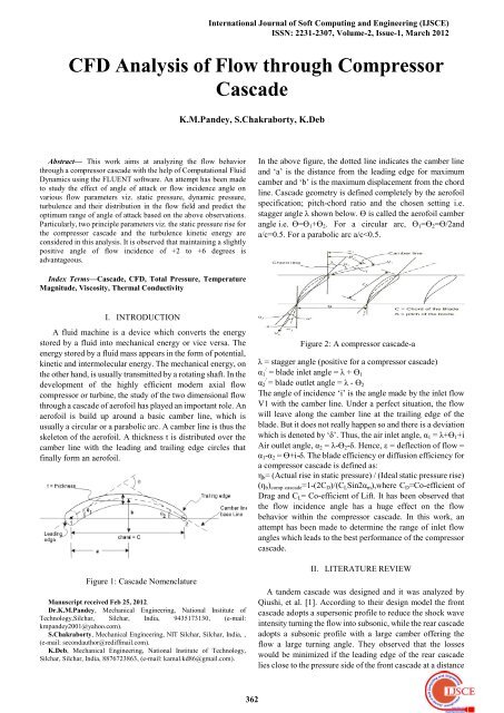
In the above figure, the dotted line indicates the camber line
and „a‟ is the distance from the leading edge for maximum
camber and „b‟ is the maximum displacement from the chord
line. Cascade geometry is defined completely by the aerofoil
specification; pitch-chord ratio and the chosen setting i.e.
stagger angle λ shown below. ϴ is called the aerofoil camber
angle i.e. ϴ=ϴ 1 +ϴ 2 . For a circular arc, ϴ 1 =ϴ 2 =ϴ/2and
a/c=0.5. For a parabolic arc a/c

CFD Analysis of Flow through Compressor Cascade
of 20% pitch in pitch-wise direction without either axial
spacing or overlapping in axial direction. Their 2D numerical
test results show that, with the inflow mach no. of 1.25 and the
turning angle of 52, the total pressure loss coefficient of the
tandem cascade reaches 0.106, and the diffusion factor 0.745,
and by adopting the finding and concerning the best relative
position of the front to the rear cascade of tandem cascade, a
high loaded fan stage with rotor tip speed of 495.32 m/s has
successfully been developed. Bakhtar and So [2] studied the
nucleating flow of steam in a cascade of supersonic blading by
the time-marching method. This investigation follows the
earlier experiment in which a case of 2D nucleating flow of
steam in a cascade was investigated, but there were some
numerical errors with the particular configuration. To discard
the errors associated with the solution they assumed the bulk
of the flow to be inviscid. They came to the conclusion that a
finer mesh can be embedded into selected regions of the basic
computational grid and its coordinates transformed if
necessary. This increases the capability of the basic technique
by increasing the accuracy in the selected region without an
undue increase in the overall computing needs. Delery &
Meauze [3] made an experimental analysis of the flow in a
highly loaded fixed compressor cascade i.e. the ISO-cascade
co-operative programme on code validation. Study was made
in a two dimensional fixed geometry to reproduce the main
physical features of the flow in a real compressor, including
strong viscous flow. The objective of them was to show how a
detailed qualification of the flow by different and
complimentary method allows to establish a consistent
physical picture of the flow in a cascade where 3D effects
plays a dominant role. The experiments were carried out in
the S5Ch transonic/supersonic wind tunnel. They found that
the large expansion over the first part of the blade suction side
is followed by a compression starting 30% downstream of the
leading edge. They also found that, if kink, followed the start
of the compression in the distribution indicative of the
presence of a laminar separation bubble then at the blade mid
portion, a rapid turning of the skin friction lines occurs and a
zone of concentration of the visualization product forms.
From their study it was possible to establish the flow topology
which contains several complex and interacting vortical
structures. Their results have been used to validate
Navier–Stokes codes and different turbulence models.
Another research work was done by Lio and Lin [4] on the
slightly perturbed two-dimensional subsonic compressible
potential flow through the cascade by direct boundary
element methods(BEMs). They have performed their work in
three BEM schemes: Scheme 1) Orthotropic medium method,
Scheme 2) Equivalent cascade method, Scheme 3)
Compressibility correction method. Using these three
schemes, they have formulated a numerical calculation of the
2D subsonic compressible potential flow through a cascade,
and used it to calculate the flow through the cascade
composed of seven identical K-7 compressor-blades. Their
calculation results were compared with each other, and with
the experimental results obtained on the same cascade in the
range of angle of attack, i = -2.5°-10 °.It has been shown that
these three direct BEM schemes lend themselves to
calculation of the 2D slightly perturbed subsonic
compressible potential flow through a cascade. Among them
the orthotropic medium method is more natural and more
trustworthy than the other two methods. State-of-the-art
prediction of the aero-elastic stability of cascades in
axial-flow turbo-machines is reviewed by another scholar
named, Forsching [5]. He worked on the comprehensive
formulation of the two- and three-dimensional classical
(unstalled) flutter problem of tuned and mistuned rotor blade
rows and bladed disc assemblies. Within the framework of
linearized analysis, a complete and generalized theory in
model form was presented, comprising the various
formulations of the cascade flutter problem distributed in
fragments throughout the literature. Brief outlines were also
made of recent advances in unsteady aerodynamic methods
for turbo-machinery aero-elastic applications. Secondly
parametric study of the classical flutter stability
characteristics of compressor and turbine cascades in
subsonic and supersonic flow had been studied by them.
Stability boundaries and dominant trends in flutter behavior
are outlined, and the significant effects of blade mistuning on
the aero-elastic stability of turbo-machine bladings were the
main features of their study. Alawa, et al. [6] had shown how
Rotor-blades‟ profile influence on a gas-turbine‟s compressor
effectiveness. Their object of the work was to establish a
relationship between changes in the incident rotor-blade angle
due to compressor blade profile distortions and the required
compressor power. This was achieved by measuring certain
performance characteristics of an operational gas-turbine.
The parameters relevant for the study at the inlet and outlet of
the compressor, as well as the inlet and outlet of turbine were
measured at the Ughelli Power Station, Delta State, Nigeria.
Performance data were obtained from the pertinent daily
log-sheets for the turbine. Design parameters were taken from
the design manuals. Theoretical predictions from computer
simulations had been compared with the corresponding
measurements. They concluded that Compressor blade profile
distortions can result in significant increases in the
compressor power required per stage as well as the decreases
in the gas turbine‟s isentropic efficiency. Compressor blade
deteriorations and distortions lead to significant reduction in
the gas-turbine‟s performance.
III. METHODOLOGY
The 2D modelling scheme was adopted in GAMBIT and it
was analysed using FLUENT. A compressor cascade model
with zero degree flow angle of incidence was designed. The
physical model is defined as follows:
Chord length
15 cm
Pitch-to-chord ratio (S/C) 0.52
Aspect ratio (H/C) 1.56
Outlet blade angle 4 degree
Stagger angle
22 degree
Number of blades 3
Operating Pressure 1 atm
Temperature
300 K
Velocity
20 m/s
Fluid
Air
The blade dimensions are taken from Ref. [7]. The model is
shown below.
363

International Journal of Soft Computing and Engineering (IJSCE)
ISSN: 2231-2307, Volume-2, Issue-1, March 2012
achieved. The results obtained for this mesh is considered to
be the best. This mesh formation was done with GAMBIT.
ssss
Figure 3: Compressor Cascade Model with boundary
types.
IV. RESULTS AND ANALYSIS
The various contours of the flow parameters such as
pressure, turbulence, velocity etc in the flow field for the
different models are given below. The red colored regions are
the regions where the properties attain their maximum values.
The blue colored regions indicate the regions where the
properties are at their minimum. The properties that were
analyzed for the various models are-
1. Static Pressure
2. Dynamic Pressure
3. Total Pressure
4. Velocity Magnitude
5. Velocity Angle
6. Turbulence Kinetic Energy
7. Effective Viscosity
8. Effective thermal Conductivity
A. Flow incidence angle:-10 degree (a=angle of attack)
Figure 4: Compressor Cascade Model - Meshed.
The flow incidence angle is determined by the x and y
velocity components which are as follows:
Table 1 : Velocity components for different flow incidence
angles.
Figure 5: Plot of Scaled Residuals (a = -10 degrees)
Flow Incidence
Angle (a)(in
degrees)
X Component of
flow direction
(cos a)
Y Component
of flow
direction (sin
a)
Figure 6: Contour of Static Pressure (a = -10 degrees)
-10 0.6691 0.7431
-6 0.6157 0.7880
-2 0.5592 0.8290
0 0.5299 0.8481
2 0.5 0.8660
Figure7: Contour of Dynamic Pressure (a = -10 degrees)
6 0.4384 0.8988
10 0.3746 0.9272
The grid independence test is done which involves
transforming the generated physical model into a mesh with
number of node points depending on the fineness of the mesh.
The various flow properties were evaluated at these node
points. The extent of accuracy of result depended to a great
extend on the fact that how fine the physical domain was
meshed. After a particular refining limit the results changes no
more. At this point it is said that grid independence is
Figure 8: Contour of Total Pressure (a = -10 degrees)
364

CFD Analysis of Flow through Compressor Cascade
Figure 9: Contour of Velocity Magnitude (a = -10 degrees)
Figure 15: Contour of Static Pressure (a = -6 degrees)
Figure 10: Contour of Velocity Angle (a = -10 degrees)
Figure 16: Contour of Dynamic Pressure (a = -6 degrees)
Figure11: Contour of Turbulence Kinetic Energy(a = -10
degrees)
Figure 17: Contour of Total Pressure (a = -6 degrees)
Figure 12: Contour of Effective Viscosity (a = -10 degrees)
Figure 18: Contour of Velocity Magnitude (a = -6 degrees)
Figure 13: Contour of Effective Thermal Conductivity (a=-10
degrees)
B. Flow incidence angle: -6 degrees
Figure 19: Contour of Velocity Angle (a = -6 degrees)
Figure 20: Contour of Turbulence Kinetic Energy (a = -6
degrees)
Figure 14: Plot of Scaled Residuals (a = -6 degrees)
365

International Journal of Soft Computing and Engineering (IJSCE)
ISSN: 2231-2307, Volume-2, Issue-1, March 2012
Figure 21: Contour of Effective Viscosity (a = -6 degrees)
Figure 27: Contour of Velocity Magnitude (a = -2 degrees)
Figure 22: Contour of Effective Thermal Conductivity (a = -6
deg.)
C. Flow incidence angle: -2 degrees
Figure 28: Contour of Velocity Angle (a = -2 degrees)
Figure 23: Plot of Scaled Residuals (a = -2 degrees)
Figure 29: Contour of Turbulence Kinetic Energy (a = -2
degrees)
Figure 30: Contour of Effective Viscosity (a = -2 degrees)
Figure 24: Contour of Static Pressure (a = -2 degrees)
Figure 25: Contour of Dynamic Pressure (a = -2 degrees)
Figure 31: Contour of Effective Thermal Conductivity (a = -2
deg.)
D. Flow incidence angle: 0 degree
Figure 26: Contour of Total Pressure (a = -2 degrees)
Figure 32: Plot of Scaled Residuals (a = 0 degree)
366

CFD Analysis of Flow through Compressor Cascade
Figure 33: Contour of Static Pressure (a = 0 degree)
Figure 40: Contour of Effective Thermal Conductivity (a = 0
degree)
E. Flow incidence angle: +2 degree
Figure 34: Contour of Dynamic Pressure (a = 0 degree)
Figure 41: Plot of Scaled Residuals (a = +2 degrees)
Figure 35: Contour of Total Pressure (a = 0 degree)
Figure 42: Contour of Static Pressure (a = +2 degrees)
Figure 36: Contour of Velocity Magnitude (a = 0 degree)
Figure 43: Contour of Dynamic Pressure (a = +2 degrees)
Figure 37: Contour of Velocity Angle (a = 0 degree)
Figure 44: Contour of Total Pressure (a = +2 degrees)
Figure 45: Contour of Velocity Magnitude (a = +2 degrees)
Figure 38: Contour of Turbulence Kinetic Energy (a = 0
degree)
Figure 46: Contour of Velocity Angle (a = +2 degrees)
Figure 39: Contour of Effective Viscosity (a = 0 degree)
367

International Journal of Soft Computing and Engineering (IJSCE)
ISSN: 2231-2307, Volume-2, Issue-1, March 2012
Figure 47: Contour of Turbulence Kinetic Energy (a = +2
degrees)
Figure 53: Contour of Total Pressure (a = +6 degrees)
Figure 48: Contour of Effective Viscosity (a = +2 degrees)
Figure 54: Contour of Velocity Magnitude (a = +6 degrees)
Figure 49: Contour of Effective Thermal Conductivity (a = +2
deg.)
F. Flow incidence angle: +6 degree
Figure 55: Contour of Velocity Angle (a = +6 degrees)
Figure 56: Contour of Turbulence Kinetic Energy (a = +6
degrees)
Figure 50: Plot of Scaled Residuals (a = +6 degrees)
Figure 57: Contour of Effective Viscosity (a = +6 degrees)
Figure 51: Contour of Static Pressure (a = +6 degrees)
Figure 58: Contour of Effective Thermal Conductivity (a= +6
deg.)
Figure 52: Contour of Dynamic Pressure (a = +6 degrees)
368

CFD Analysis of Flow through Compressor Cascade
G. Flow incidence angle: +10 degree
Figure 59: Plot of Scaled Residuals (a = +10 degrees)
Figure 65: Contour of Turbulence Kinetic Energy (a = +10
degrees)
Figure 66: Contour of Effective Viscosity (a = +10 degrees)
Figure 60: Contour of Static Pressure (a = +10 degrees)
Figure 61: Contour of Dynamic Pressure (a = +10 degrees)
Figure 62: Contour of Total Pressure (a = +10 degrees)
Figure 63: Contour of Velocity Magnitude (a = +10 degrees)
Fig. 67: Contour of Effective Thermal Conductivity (a = +10
degrees)
V. CONCLUSION
It is observed from these contours that the static pressure
for a compressor cascade increases along the cascade flow
field, while the dynamic pressure and velocity decreases. The
total pressure shows a layer-by-layer pattern over the blade
profile. The velocity angle at any point in the flow field
indicates the direction in which the flow is flowing at that
point. The turbulence kinetic energy shows a decreasing value
from the inlet. It can be noted that the effective viscosity and
effective thermal conductivity is higher at regions of higher
turbulence. This can be attributed to the fact that due to
turbulence, a greater inter-mixing of the fluid molecules occur
leading to increased resistance to flow, increasing the heat
conductivity at the same time.
A comparison of the contours of static pressure for the
different inlet flow angles gives the following values:
Table 2: Static Pressure rise for different flow incidence
angles.
Flow Incidence Angle (in Static Pressure Rise (bar)
degree)
Figure 64: Contour of Velocity Angle (a = +10 degrees)
-10 121.223
-6 123.247
-2 141.156
0 141.552
2 142.39
6 137.327
10 127.948
369

Plotting these values, a bell shaped curve is obtained which
show its peak value at around +2 degrees. This is shown
below.
International Journal of Soft Computing and Engineering (IJSCE)
ISSN: 2231-2307, Volume-2, Issue-1, March 2012
Static Pressure Rise
145
140
135
130
Y-Values
125
120
-20 -10 0 10 20
Figure 68: Plot of Static Pressure Rise (in bar) v/s Flow
Incidence Angle (in degrees)
Greater the pressure rise, more is the work done by the
compressor cascade with the same input parameters. A
comparison of the Turbulence Kinetic Energy shows the
following:
Figure 69: Comparison of Turbulence Kinetic Energy for
Compressor Cascade in sequence of -10, -6, -2, 0, +2, +4, +6
and +10.
It can be noticed that the Turbulence Kinetic Energy shows a
gradual decrease towards positive angles of attack,
particularly in the range of +2 to +6 degrees. Thus
maintaining a positive flow incidence angle in the range of +2
to +6 degrees would be advantageous.
VI. SCOPE FOR FUTURE WORK
The analysis done on the cascade models falls short of a
more realistic evaluation of flow parameters due to the
absence of the stator as applicable in turbo-machines. Due to
this, the inlet flow conditions more or less deviates from the
actual ones. Also, a three dimensional model of the cascade
will be able to simulate the flow conditions in a more effective
and realistic manner. The computational results should be
validated by experimental work performed under controlled
conditions.
370

CFD Analysis of Flow through Compressor Cascade
Hence future work in this direction, which includes a
complete stage, involving a stator and a rotor, designed in the
three dimensions, can provide a better ground for analyzing
the flow through a cascade followed by experimental work to
validate the computational results.
VII. Acknowledgement
The authors acknowledge the financial help
provided by AICTE from the project AICTE:
8023/RID/BOIII/NCP(21) 2007-2008 .The Project id at IIT
Guwahati is ME/P/USD/4.
REFERENCES
[1] Li Qiushi, Wu Hong, and Zhou Sheng, “Application Of Tandem
Cascade To Design Of Fan With Supersonic Flow”, Chinese
Journal of Aeronautics, Elsevier; 23(2010):9-14
[2] F.Bakhtar and K.S So, “A Study Of Nucleating Flow Of Steam
In A Cascade Of Supersonic Blading By The Time-Marching
Method”, International Journal Of Heat & Fluid Flow, Vol. 12,
No.1,Butterworth-Heinemann,1991.
[3] J. Delery & G. Meauze, “A Detailed Experimental Analysis Of
The Flow In A Highly Loaded Fixed Compressor Cascade: The
Iso-Cascade Co-Operative Programme On Code Validation”,
Aerospace Science & Technology 7,Elsevier;2009:1-9.
[4] A.X. Lio and C.X. Lin, “Three BEM Schemes For The
Calculating Of Subsonic Compressible Plane Cascade Flow”,
Engineering Analysis with Boundary Elements 11; 1993 :
25-32.
[5] H. Forsching, “Aero-elastic stability of Cascades in
Turbo-Machinery”, Prog. Aerospace Science, Vol. 30
Pergamon;1994: 213-216.
[6] B.T. Lebele Alawa, H.I. Hart, S.O.T. Ogaji, S.D. Probert, “Rotor
Blades‟ Profile Influence On A Gas Turbine‟s Compressor
Effectiveness”, Applied Energy 85 , Elsevier; 2008, 494-505.
[7] U. K. Saha, B. Roy, “Experimental Investigations on Tandem
Compressor Cascade Performance at Low Speeds”,
Experimental Thermal and Fluid Science, Elsevier; 1997;
14:263-276.
S.Chakraborty has completed his B.Tech from NIT Silchar in 2011.
K.Deb is currently doing his
M.Tech from NIT Silchar, he
also qualified GATE in
2011,his research interests are
CFD, Combustion and
Gasification.
Dr. K.M.Pandey did his B.Tech in 1980 from BHUIT Varanasi, India in
1980.He obtained M.Tech. in heat power in 1987 .He received PhD in
Mechanical Engineering in 1994 from IIT Kanpur. He has published and
presented more than 200 papers in International & National Conferences
and Journals. Currently he is working as Professor of the Mechanical
.Engineering Department, National Institute of Technology,
Silchar,Assam, India..He also served thedepartment in the capacity of head
from July 07 to 13 July 2010. He has alsoworked as faculty consultant
in Colombo Plan Staff College, Manila, Philippines as seconded faculty
from Government of India. His research interest areas are the
following; Combustion, High Speed Flows,Technical Education, Fuzzy
Logic and Neural Networks , Heat Transfer, Internal Combustion Engines,
Human Resource Management, Gas Dynamics and Numerical Simulations
in CFD area from Commercial Software‟s. Currently he is also working as
Dean, Faculty Welfare at NIT Silchar, Assam, India.
Email:kmpandey2001@yahoo.com.
371