Long solitary internal waves in stable stratifications
Long solitary internal waves in stable stratifications
Long solitary internal waves in stable stratifications

Create successful ePaper yourself
Turn your PDF publications into a flip-book with our unique Google optimized e-Paper software.
Nonl<strong>in</strong>ear Processes <strong>in</strong> Geophysics (2004) 11: 165–180<br />
SRef-ID: 1607-7946/npg/2004-11-165<br />
Nonl<strong>in</strong>ear Processes<br />
<strong>in</strong> Geophysics<br />
© European Geosciences Union 2004<br />
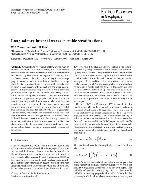
<strong>Long</strong> <strong>solitary</strong> <strong><strong>in</strong>ternal</strong> <strong>waves</strong> <strong>in</strong> <strong>stable</strong> <strong>stratifications</strong><br />
W. B. Zimmerman 1 and J. M. Rees 2<br />
1 Department of Chemical and Process Eng<strong>in</strong>eer<strong>in</strong>g, University of Sheffield, Sheffield S1 3JD, UK<br />
2 Department of Applied Mathematics, University of Sheffield, Sheffield S3 7RH, UK<br />
Received: 2 December 2003 – Accepted: 21 January 2004 – Published: 14 April 2004<br />
Abstract. Observations of <strong><strong>in</strong>ternal</strong> <strong>solitary</strong> <strong>waves</strong> over an<br />
antarctic ice shelf (Rees and Rottman, 1994) demonstrate<br />
that even large amplitude disturbances have wavelengths that<br />
are bounded by simple heuristic arguments follow<strong>in</strong>g from<br />
the Scorer parameter based on l<strong>in</strong>ear theory for wave trapp<strong>in</strong>g.<br />
Classical weak nonl<strong>in</strong>ear theories that have been applied<br />
to <strong>stable</strong> <strong>stratifications</strong> all beg<strong>in</strong> with perturbations<br />
of simple long <strong>waves</strong>, with corrections for weak nonl<strong>in</strong>earity<br />
and dispersion result<strong>in</strong>g <strong>in</strong> nonl<strong>in</strong>ear wave equations<br />
(Korteweg-deVries (KdV) or Benjam<strong>in</strong>-Davis-Ono) that admit<br />
localized propagat<strong>in</strong>g solutions. It is shown that these<br />
theories are apparently <strong>in</strong>appropriate when the Scorer parameter,<br />
which gives the lowest wavenumber that does not<br />
radiate vertically, is positive. In this paper, a new nonl<strong>in</strong>ear<br />
evolution equation is derived for an arbitrary wave packet<br />
thus <strong>in</strong>clud<strong>in</strong>g one bounded below by the Scorer parameter.<br />
The new theory shows that <strong>solitary</strong> <strong><strong>in</strong>ternal</strong> <strong>waves</strong> excited <strong>in</strong><br />
high Richardson number waveguides are predicted to have a<br />
halfwidth <strong>in</strong>versely proportional to the Scorer parameter, <strong>in</strong><br />
agreement with atmospheric observations. A localized analytic<br />
solution for the new wave equation is demonstrated,<br />
and its soliton-like properties are demonstrated by numerical<br />
simulation.<br />
1 Introduction<br />
Chemical eng<strong>in</strong>eer<strong>in</strong>g abounds with unit operations where<br />
<strong>solitary</strong> <strong>waves</strong> can be <strong>in</strong>duced. Film flows, especially <strong>in</strong> condensers<br />
and distillation columns, give rise to sheared, <strong>stable</strong><br />
<strong>stratifications</strong> where <strong>solitary</strong> <strong>waves</strong> can be <strong>in</strong>duced by<br />
mass transfer (Hewakandamby and Zimmerman, 2003) or<br />
heat transfer effects that are driven by surface tension gradients.<br />
In this paper, motivated by recent studies of surfactant<br />
spread<strong>in</strong>g on sheared, <strong>stable</strong> <strong>stratifications</strong> and observations<br />
<strong>in</strong> the <strong>stable</strong> Antarctic boundary layer (Rees and Rottman,<br />
Correspondence to: W. B. Zimmerman<br />
(w.zimmerman@shef.ac.uk)<br />
1994), we revisit the classical analysis lead<strong>in</strong>g to the conclusion<br />
that large amplitude <strong>waves</strong> can be <strong>in</strong>duced <strong>in</strong> the <strong>in</strong>f<strong>in</strong>ity<br />
long limit. Scorer (1949) po<strong>in</strong>ted out that longer <strong>waves</strong><br />
than a particular value selected by the shear and stratification<br />
profiles, radiate vertically, and thus are not trapped by the<br />
waveguide. This condition is the modification due to shear<br />
of the classical Brunt-Väisälä frequencyfor vertical radiation<br />
of <strong>waves</strong> <strong>in</strong> a purely stratified fluid. In this paper, we take<br />
<strong>in</strong>to account this limitation and pose a derivation of the nonl<strong>in</strong>ear<br />
evolution equation (NEE) which reduces to the classical<br />
Korteweg-de Vries equation <strong>in</strong> the case that the Scorer<br />
wavenumber approaches zero so that <strong>in</strong>f<strong>in</strong>itely long <strong>waves</strong><br />
are trapped.<br />
Benney (1966) and Benjam<strong>in</strong> (1966) <strong>in</strong>dependently derived<br />
the first NEE for large amplitude <strong>solitary</strong> disturbances<br />
<strong>in</strong> a <strong>stable</strong> stratification with shear flow. They both assumed<br />
weak nonl<strong>in</strong>earity and weak dispersion due to a long wave<br />
approximation. The derived NEE, which applies equally to<br />
either temperature or streamfunction disturbances, takes the<br />
form of a Korteweg-deVries (KdV) equation, with coefficients<br />
that depend on both the conditions of the waveguide<br />
(functionals of the stratification and shear profiles) and on<br />
the characteristics of the disturbance itself (wavelength and<br />
amplitude):<br />
∂A<br />
∂t<br />
+ (c + A) ∂A<br />
∂x + σ ∂3 A<br />
∂x 3 = 0 . (1)<br />
This has the solution that the amplitude A, at time t and position<br />
x, is<br />
( (A0 ) 1/2<br />
A = 3A 0 sech 2 (x − (c + A 0 )t))<br />
(2)<br />
4σ<br />
where A 0 is the amplitude of the <strong>in</strong>itial disturbance, c the<br />
phase velocity of <strong>in</strong>f<strong>in</strong>itely long <strong>waves</strong>, and σ = cH 2 /6 is the<br />
parameter measur<strong>in</strong>g dispersion. H is the layer depth. The<br />
halfwidth of the <strong>solitary</strong> wave is (A 0 /16σ ) −1/2 . Because this<br />
halfwidth is <strong>in</strong>versely proportional to √ σ , it follows that the<br />
wavelength of a localised disturbance depends <strong>in</strong>versely on
166 W. B. Zimmerman and J. M. Rees: <strong>Long</strong> <strong>solitary</strong> <strong>waves</strong><br />
the spectral width of the wave packet that characterizes the<br />
Fourier power spectrum of the disturbance.<br />
The KdV theory proposed by Benney and Benjam<strong>in</strong> is<br />
robust, with many applications <strong>in</strong> atmospheric and oceanographic<br />
analysis, e.g. Doviak et al. (1991). Nevertheless,<br />
there is a fundamental problem with the derivation of the<br />
KdV theory from the <strong>in</strong>f<strong>in</strong>itely long wave limit. Essentially,<br />
<strong>in</strong> some circumstances, the waveguide will be depleted of<br />
wave energy <strong>in</strong> long scales. This is described more fully below.<br />
Benney’s derivation beg<strong>in</strong>s with a l<strong>in</strong>ear wave equation<br />
that to lead<strong>in</strong>g order is a simple wave of <strong>in</strong>f<strong>in</strong>itely long wavelength,<br />
satisfy<strong>in</strong>g:<br />
∂A<br />
∂t<br />
+ c ∂A<br />
∂x = 0 (3)<br />
Scorer (1949), however, considers modified Brunt-Väisälä<br />
vertical buoyancy <strong>waves</strong> <strong>in</strong> the presence of shear flow. He<br />
concludes that wave energy is only trapped if it is conf<strong>in</strong>ed<br />
to wavenumbers k that are greater than the Scorer parameter<br />
L def<strong>in</strong>ed here:<br />
L 2 = N 2 1<br />
(û ) 2<br />
− (û ) d2 û<br />
− ν − ν dy 2 (4)<br />
N is the Brunt-Väisälä frequency, ν is the phase velocity,<br />
and û (y) is the background shear profile, which is assumed<br />
steady before and after the passage of the disturbance.<br />
Wave energy can radiate vertically out of the waveguide as<br />
Brunt-Väisälä <strong>waves</strong> if the wavenumber of the disturbance<br />
is smaller than L. Scorer (1949), showed that the Fourier<br />
component of the vertical velocity ŵ k satisfies <strong>in</strong> the l<strong>in</strong>ear<br />
approximation:<br />
d 2 ŵ k<br />
dy 2 + (<br />
L 2 − k 2) ŵ k = 0 . (5)<br />
y is the vertical coord<strong>in</strong>ate and k is the wavenumber of the<br />
disturbance. Scorer showed that when L 2 decreases with<br />
height, energy can be trapped at low levels. More generally,<br />
with<strong>in</strong> <strong>in</strong> any waveguide, if L 2 > k 2 , Eq. (5) admits oscillatory<br />
solutions that radiate vertically as Brunt-Väisälä <strong>waves</strong>.<br />
When L 2 < k 2 , one solution of Eq. (5) is a bound-state, i.e.<br />
energy is trapped <strong>in</strong> the waveguide and can only propagate<br />
with<strong>in</strong> the waveguide. The other solution to Eq. (5) <strong>in</strong> this<br />
case is exponential growth far away from the waveguide,<br />
which is rejected as aphysical.<br />
The wavelength of <strong>solitary</strong> disturbances over an Antarctic<br />
ice shelf has been discussed by Rees and Rottman (1994).<br />
These authors provided empirical evidence show<strong>in</strong>g that<br />
even large amplitude disturbances have halfwidths that agree<br />
remarkably well with the l<strong>in</strong>ear Taylor-Goldste<strong>in</strong> theory described<br />
by Scorer (1949). This is a surpris<strong>in</strong>g result <strong>in</strong> that for<br />
the large amplitude disturbances that were reported by Rees<br />
and Rottman (1994), nonl<strong>in</strong>ear effects are important and l<strong>in</strong>ear<br />
theory would be expected to fail. They cited Scorer’s argument<br />
that l<strong>in</strong>ear <strong>waves</strong> longer than wavenumber L would<br />
radiate vertically out of the waveguide. S<strong>in</strong>ce wave energy<br />
at scales shorter than the Scorer wavenumber L are trapped<br />
<strong>in</strong> the waveguide, it is not at first clear why large amplitude<br />
<strong>solitary</strong> disturbances exhibit the Scorer wavenumber.<br />
Ursell (1953) resolved a long stand<strong>in</strong>g paradox <strong>in</strong> the theory<br />
of <strong>solitary</strong> surface gravity <strong>waves</strong> by co<strong>in</strong><strong>in</strong>g a new dimensionless<br />
number Ur = A 0 L 2 /H 3 = ε/µ 2 , the ratio of two dimensionless<br />
numbers. ε = A 0 /H is the ratio of the maximum<br />
streamfunction displacement to the height H of the waveguide.<br />
µ = H/L is the ratio of the height of the waveguide<br />
to the expected wavelength L of the long wave disturbance.<br />
Thus, ε and µ are properties of the resultant wave generated<br />
from some <strong>in</strong>itial disturbance to the waveguide. S<strong>in</strong>ce the<br />
formation of a <strong>solitary</strong> wave may occur after a comb<strong>in</strong>ation<br />
of the nonl<strong>in</strong>ear break<strong>in</strong>g of the <strong>in</strong>itial disturbance or the dispersion<br />
of different components, the length scales of the <strong>in</strong>itial<br />
conditions may have little bear<strong>in</strong>g on the resultant wave.<br />
Thus, the description of <strong>solitary</strong> wave motion by the parameters<br />
µ and ε ignores the history of its formation. Ursell suggested<br />
that when Ur ∼ 1, with both ε ≪ 1 and µ ≪ 1, <strong>solitary</strong><br />
<strong>waves</strong> of permanent form can propagate. In fact, this<br />
argument previously appeared <strong>in</strong> the pioneer<strong>in</strong>g papers of<br />
(Bouss<strong>in</strong>esq, 1871a,b, 1872) and was understood earlier by<br />
Lord Rayleigh (Rayleigh, 1876). It should be noted, that <strong>in</strong><br />
def<strong>in</strong><strong>in</strong>g µ and ε as above, the <strong>solitary</strong> wave is presupposed<br />
to exist. On dimensional analysis grounds, µ and ε are <strong>in</strong>dependent<br />
parameters. The Ursell hypothesis relat<strong>in</strong>g the two<br />
follows from the stronger constra<strong>in</strong>t that the <strong>solitary</strong> wave<br />
should have permanent form. The specific functional relationship<br />
that Ursell proposed was physically motivated by the<br />
mechanism ma<strong>in</strong>ta<strong>in</strong><strong>in</strong>g permanent form–nonl<strong>in</strong>ear steepen<strong>in</strong>g<br />
balanc<strong>in</strong>g wave dispersion.<br />
Internal <strong>solitary</strong> <strong>waves</strong> may propagate <strong>in</strong> a waveguide of<br />
a stratified fluid layer, with and without shear. However, the<br />
<strong>in</strong>clusion of shear <strong>in</strong>troduces a free parameter, the Richardson<br />
number Ri, the ratio of buoyancy to shear forces, which<br />
affects the balance of nonl<strong>in</strong>earity and dispersion <strong>in</strong> wave<br />
pro- pagation. Dimensional analysis, along with the constra<strong>in</strong>t<br />
that the waveform be permanent, results <strong>in</strong> the functional<br />
relationship ε = f (µ, Ri). The form of this functional<br />
relationship should be based on account<strong>in</strong>g for the relative<br />
strength of shear and stratification <strong>in</strong> ma<strong>in</strong>ta<strong>in</strong><strong>in</strong>g the balance<br />
between nonl<strong>in</strong>earity and dispersion <strong>in</strong> the propagation of a<br />
wave of permanent form. It follows that the wavelength that<br />
should be selected <strong>in</strong> the long time asymptotic state should<br />
be that with weakest dispersion balanc<strong>in</strong>g weak nonl<strong>in</strong>earity<br />
– so that neither mechanism is strong enough to break up<br />
the permanent form. Thus, <strong>in</strong> the time asymptotic state, the<br />
wavelength should be as long as possible. The longest wavelength<br />
admissible, therefore, <strong>in</strong> a sheared, stratified flow, is<br />
identified with the Scorer wavenumber L.<br />
Benney (1966) and Benjam<strong>in</strong> (1966) <strong>in</strong>dependently<br />
treated the weakly nonl<strong>in</strong>ear shallow layer approximation,<br />
show<strong>in</strong>g that disturbances travel accord<strong>in</strong>g to the KortewegdeVries<br />
equation if the bound<strong>in</strong>g surfaces of the layer are material<br />
surfaces (no flux of momentum vertically, no horizontal<br />
stress). This assumption is not always compatible with a<br />
cont<strong>in</strong>uously stratified fluid where a small stratum forms the<br />
waveguide, s<strong>in</strong>ce <strong>waves</strong> longer than the Scorer wavenumber
W. B. Zimmerman and J. M. Rees: <strong>Long</strong> <strong>solitary</strong> <strong>waves</strong> 167<br />
Fig. 1. Temperature (re-based) and vertical velocity of a <strong>solitary</strong><br />
disturbance observed at Halley Station by the British Antarctic Survey<br />
on 6 June 1986 at a height of 16 m. Measurements were made<br />
us<strong>in</strong>g a sonic anemometer and were recorded at 20 Hz.<br />
Fig. 2. Temperature (re-based) and vertical velocity of a <strong>solitary</strong><br />
disturbance observed at Halley Station by the British Antarctic Survey<br />
on 14 August 1986.<br />
L radiate vertically. From the def<strong>in</strong>ition (4), there are two<br />
dist<strong>in</strong>ct cases: L 2 > 0, where longer <strong>waves</strong> radiate vertically;<br />
L 2 < 0, where all wavenumbers are trapped. In this latter<br />
case, the lack of radiation vertically is consistent with the<br />
boundary conditions of the model adopted by Benney (1966)<br />
and Benjam<strong>in</strong> (1966) lead<strong>in</strong>g to the KdV theory–parallel, impenetrable<br />
stress-free surfaces. Although <strong>in</strong> this paper the<br />
focus is on wave propagation with L 2 > 0, observations of<br />
both cases <strong>in</strong> the STABLE data sets of the British Antarctic<br />
Survey are reported.<br />
When L 2 > 0, from the analysis of Scorer, it is clear that<br />
the k = 0 long wave limit is <strong>in</strong>accessible when shear and<br />
stratification establish a waveguide that is one stratum of the<br />
deeper fluid, s<strong>in</strong>ce all wavenumbers smaller than |L| will radiate<br />
vertically. Thus, long times after the <strong>in</strong>itial disturbance<br />
show depletion <strong>in</strong> the horizontal waveguide of energy <strong>in</strong> the<br />
k ∈ [0, |L|) band. However, for wavenumbers greater than<br />
|L|, the upper and lower surfaces of waveguide do act as material<br />
surfaces, s<strong>in</strong>ce these wavenumbers are trapped. It follows<br />
that the proper nonl<strong>in</strong>earisation of the l<strong>in</strong>ear dispersive<br />
<strong>waves</strong> is bounded below <strong>in</strong> wavenumber space by |L|, and<br />
is, therefore, dist<strong>in</strong>ctly different from the analysis of Benney<br />
(1966) and Benjam<strong>in</strong> (1966), which start from <strong>in</strong>f<strong>in</strong>itely<br />
long <strong>waves</strong> <strong>in</strong> the lead<strong>in</strong>g order separation condition (3). In<br />
the theory that follows, the basic disturbance is taken to be a<br />
harmonic wave with wavenumber k 2 > L 2 , and the first solvability<br />
condition leads to an NEE similar <strong>in</strong> form to the KdV<br />
equation.<br />
The paper is organised as follows: In Sect. 2, two wave<br />
events with L 2 of different signs are reported from the British<br />
Antarctic Survey STABLE data sets (K<strong>in</strong>g and Anderson,<br />
1988). In Sect. 3, a KdV-like theory for arbitrary wavelength<br />
basic disturbances is derived. When L 2 > 0, the theory is<br />
only applicable for nearly monochromatic disturbances. For<br />
L 2 < 0, the trapp<strong>in</strong>g <strong>in</strong> the waveguide is complete and the<br />
theory is generally applicable. Section 4 discusses the re-<br />
sults of the theory, demonstrat<strong>in</strong>g an analytic solution to the<br />
full NEE. Furthermore, the prediction that the halfwidth of<br />
the <strong>solitary</strong> wave by the Scorer parameter, which is demonstrated<br />
<strong>in</strong> Sect. 2 on the STABLE data set, holds theoretically<br />
<strong>in</strong> large Ri waveguides. Section 6 explores numerical simulations<br />
of the NEE, which provide some evidence of solitonic<br />
behaviour for the dynamics of overtak<strong>in</strong>g collisions <strong>in</strong>volv<strong>in</strong>g<br />
<strong>solitary</strong> wave solutions to the NEE. In Sect. 6, conclusions<br />
are drawn.<br />
2 Observations of atmospheric <strong>solitary</strong> disturbances <strong>in</strong><br />
the Antarctic<br />
As a result of strong radiative cool<strong>in</strong>g at the earth’s surface<br />
dur<strong>in</strong>g the Antarctic w<strong>in</strong>ter, a strong, long-last<strong>in</strong>g, stably<br />
stratified atmospheric boundary layer is established at Halley<br />
IV station, Antarctica (75.6 ◦ S, 26.7 ◦ W). Halley IV station<br />
is situated on the Brunt Ice Shelf which provides a uniform<br />
fetch of 10–40 km <strong>in</strong> all directions. Thus the site serves<br />
as an “ideal” natural laboratory for the study of the <strong>stable</strong><br />
atmospheric boundary layer and any wave-like structures it<br />
may support. The British Antarctic Survey have compiled<br />
a database of meteorological measurements from Halley IV<br />
station dur<strong>in</strong>g their STABLE project for the purpose of develop<strong>in</strong>g<br />
a climatology of gravity wave activity <strong>in</strong> the boundary<br />
layer (K<strong>in</strong>g and Anderson, 1988; Rees, 1991; Rees et al.,<br />
2000). The <strong>solitary</strong> large amplitude disturbances reported<br />
here are typical examples of several observations <strong>in</strong> the data<br />
set. The meteorological data recorded <strong>in</strong> the 1986 STABLE<br />
project <strong>in</strong>cluded w<strong>in</strong>d speed, w<strong>in</strong>d direction, and temperature<br />
on a 32 m mast, with measurements at six heights.<br />
Figure 1 shows the temperature fluctuation about an arbitrary<br />
mean and vertical velocity of a wave event recorded<br />
6 June 1986 at a height of 16 m. By eye, it is apparent that the<br />
fundamental assumption of both the KdV theory and BDO
168 W. B. Zimmerman and J. M. Rees: <strong>Long</strong> <strong>solitary</strong> <strong>waves</strong><br />
Fig. 3. Computed shear profile, temperature, Richardson number<br />
and Scorer parameter of the observed <strong>solitary</strong> disturbance at Halley<br />
Station by the British Antarctic Survey on 6 June 1986, at 100 s<br />
(after the wave passed) with the orig<strong>in</strong> of time def<strong>in</strong>ed <strong>in</strong> Fig. 2,<br />
follow<strong>in</strong>g Rees and Rottman.<br />
Fig. 4. Computed speed, temperature, Richardson number and<br />
Scorer parameter of the observed <strong>solitary</strong> disturbance at Halley Station<br />
by the British Antarctic Survey on 14 August 1986, at 300 s<br />
(after the wave passed) with the orig<strong>in</strong> of time def<strong>in</strong>ed <strong>in</strong> Fig. 3,<br />
follow<strong>in</strong>g Rees and Rottman.<br />
theory is approximately satisfied, i.e. that the streamfunction<br />
and temperature field T have the same disturbance waveform<br />
<strong>in</strong> the horizontal waveguide. S<strong>in</strong>ce vertical velocity w is the<br />
expressed through a spatial derivative of the streamfunction,<br />
this can be modelled by separation of variables:<br />
T = A (x, t) θ (y) + O(ε)<br />
w = ∂A φ (y) + O(ε) (6)<br />
∂x<br />
For simple long <strong>waves</strong>, to a first approximation<br />
∂A<br />
∂x = −1 ∂A<br />
c ∂t<br />
S<strong>in</strong>ce it appears that the vertical velocity <strong>in</strong> Fig. 1 is roughly<br />
proportional to the negative time derivative of the disturbance<br />
temperature field, it is consistent with the premise that either<br />
weakly nonl<strong>in</strong>ear theory (KdV or BDO) applies.<br />
Figure 2 is from a different wave event which occurred on<br />
14 August 1986. Although the qualitative picture rema<strong>in</strong>s<br />
very similar to the event on 6 June 1986, there is a fundamental<br />
difference <strong>in</strong> the vertical structure of the waveguides.<br />
Figure 3 shows fitted profiles for the background shear flow<br />
and temperature, with the Richardson number and Scorer parameter<br />
computed from them. The details of the modell<strong>in</strong>g of<br />
the data were presented by Rees and Rottman (1994). What<br />
is apparent from the Richardson number plot is that there is<br />
(7)<br />
a stratum of very strong stratification at a low level (circa<br />
10 m) subtended by upper and lower regions of strong shear.<br />
In the vic<strong>in</strong>ity of this stratum, the Scorer parameter has an<br />
<strong><strong>in</strong>ternal</strong> maximum which is greater than zero, the condition<br />
under which Scorer argued that energy could be trapped at<br />
higher wavenumbers at low levels. Those authors noted that<br />
for this event, the wavelength of <strong>waves</strong> at the Scorer cut-off<br />
is approximately:<br />
2π<br />
√<br />
0.001 m −2 ≈ 200 m<br />
Rough statistics on the <strong>solitary</strong> disturbance give duration 50 s<br />
and phase velocity 4.5 m/s, i.e. a wavelength of 225 m. Given<br />
the accuracy at which the duration can be estimated, say<br />
between 40 s (wavelength 180 m) and 50 s, this is quite astonish<strong>in</strong>g<br />
agreement. Nor is this an isolated event. The<br />
Scorer parameter is negative below 5 m, <strong>in</strong>dicat<strong>in</strong>g that all<br />
wavenumbers k ≥ 0 are trapped below this height.<br />
Figure 4 gives the equivalent observed and derived features<br />
for the wave event on 14 August 1986. In this <strong>in</strong>stance,<br />
the stratum for which stratification dom<strong>in</strong>ates shear is both<br />
broader and weaker. The Scorer parameter is negative <strong>in</strong> this<br />
stratum, <strong>in</strong>dicat<strong>in</strong>g that all wavenumbers k ≥ 0 are trapped.<br />
Estimates of a duration of 33 s and phase velocity of 7.0 m/s<br />
give a similar wavelength of 210 m.<br />
The events reported here lead to the question of whether<br />
there exists a selection mechanism for the wavelength of
W. B. Zimmerman and J. M. Rees: <strong>Long</strong> <strong>solitary</strong> <strong>waves</strong> 169<br />
<strong>solitary</strong> <strong><strong>in</strong>ternal</strong> <strong>waves</strong>. The focus on the Scorer parameter,<br />
given the <strong>in</strong>dication that when L 2 > 0, there is apparent<br />
correlation with observed wavelengths, begs the question of<br />
the mechanism of wavelength selection. Further, if there is<br />
a wavelength selection for waveguides with L 2 > 0, is there<br />
none for L 2 < 0? The theory developed <strong>in</strong> the next section is<br />
motivated by these questions.<br />
3 Model system<br />
3.1 Equations and scal<strong>in</strong>g<br />
Consider a fluid layer bounded above and below by parallel<br />
material surfaces. The upper material surface is constra<strong>in</strong>ed<br />
to move at velocity U = γ H , where γ is the shear rate, and<br />
is held at constant temperature T = 1. The lower is held at<br />
T = 0 and at rest. As the model that is proposed is Galilean<br />
<strong>in</strong>variant, an arbitrary uniform w<strong>in</strong>d component could be <strong>in</strong>cluded<br />
without loss of generality. The fluid is <strong>in</strong>viscid and<br />
nonconduct<strong>in</strong>g. All lengths are scaled by H , velocity by<br />
U, and time by H/U. The flow is assumed to be twodimensional<br />
and divergence free, thus expressible through<br />
a streamfunction, (u, v) = ( )<br />
y , − x . Scalar transport is<br />
modelled as convection only:<br />
T t + y T x − x T y = 0 (8)<br />
A Bouss<strong>in</strong>esq fluid is assumed, with density l<strong>in</strong>early related<br />
to temperature. The dimensionless density is ρ = 1−βT ,<br />
where β is the dimensionless group formed from the coefficient<br />
of thermal expansion β ∗ , the unscaled temperature<br />
difference between the upper and lower surfaces T , and<br />
ρ 0 , the density of the fluid at the reference temperature of the<br />
lower surface. Namely, β = β ∗ T /ρ 0 .<br />
Vorticity ω = − ∇ 2 is transported by<br />
0 = RiT x + [ yt + y xy − x yy<br />
]y<br />
+ [ xt + y xx − x xy<br />
]x<br />
(9)<br />
which is the curl of the Bouss<strong>in</strong>esq momentum equation. The<br />
Richardson number is a measure of the relative importance<br />
of buoyant forces to shear forces, Ri = βgH /U 2 = N 2 /γ 2 .<br />
The assumption of a Bouss<strong>in</strong>esq fluid is that the velocity field<br />
is divergence-free, β ≡ 0, and the Ri rema<strong>in</strong>s f<strong>in</strong>ite. No penetration<br />
(and stress free) and fixed temperature boundary conditions<br />
are imposed:<br />
| y=0 = T | y=0 = 0<br />
| y=1 = T | y=1 = 1 (10)<br />
Because there is no dynamic boundary condition, pressure<br />
was elim<strong>in</strong>ated, result<strong>in</strong>g <strong>in</strong> the momentum (9).<br />
3.2 Wave disturbances of permanent form<br />
Generally, the flow and temperature fields can be arbitrarily<br />
decomposed <strong>in</strong>to background fields and disturbance fields.<br />
To make the procedure determ<strong>in</strong>istic, the assumption is made<br />
that the disturbance field has zero mean <strong>in</strong> some sense. The<br />
sense adopted here is that the background fields are timeaveraged<br />
and thus steady. Further, the background fields are<br />
prescribed and <strong>in</strong>dependent of the horizontal x-coord<strong>in</strong>ate.<br />
T = ˆT (y) + εT (x, y, t)<br />
= ˆψ (y) + εψ (x, y, t) (11)<br />
ε = A 0 /h is the dimensionless characteristic size of the disturbance<br />
fields, where A 0 is the maximum value of the <strong>in</strong>itial<br />
disturbance. For convenience, the follow<strong>in</strong>g representative<br />
case of l<strong>in</strong>ear shear and stratification are considered:<br />
ˆT = y<br />
ˆψ = y2<br />
2<br />
(12)<br />
S<strong>in</strong>ce it is the long time waveform which is required, and it<br />
is expected that that the form of solution will be steady <strong>in</strong> a<br />
the frame of reference of the phase velocity ν, the follow<strong>in</strong>g<br />
coord<strong>in</strong>ate transform is made:<br />
( ) ( )<br />
x ξ = x − νt<br />
→<br />
;<br />
t τ = εt<br />
( ∂<br />
∂x<br />
=<br />
∂ξ<br />
∂<br />
∂<br />
∂t<br />
= ε ∂<br />
∂τ − ν ∂<br />
∂ξ<br />
)<br />
(13)<br />
It is anticipated that the approach to a wave of permanent<br />
form occurs over a slow time scale. Substitut<strong>in</strong>g Eq. (11)<br />
<strong>in</strong>to Eqs. (8) and (9) yields<br />
T ξ (y − ν) − ψ ξ = ε ( −θ τ + ψ ξ T y − ψ y T ξ<br />
)<br />
[<br />
ψyξ (y − ν) − ψ ξ<br />
]<br />
y + RiT ξ + [ ψ ξξ (y − ν) ] ξ<br />
= ε<br />
(−ψ yτ + [ ] )<br />
ψ ξ ψ yy − ψ y ψ ξy y − ψ ξξτ<br />
( [ψξ ] )<br />
+ ε ψ ξy − ψ y ψ ξξ<br />
ξ<br />
(14)<br />
If ε ≪ 1, it is quite natural to consider the vanish<strong>in</strong>g amplitude<br />
limit of ε = 0. The basic disturbance T (0) , ψ (0) satisfies<br />
T (0)<br />
ξ<br />
(y − ν) − ψ (0)<br />
ξ<br />
= 0<br />
[<br />
]<br />
ψ (0)<br />
(0)<br />
yξ<br />
(y − ν) − ψ(0)<br />
ξ<br />
+ RiT<br />
y<br />
ξ<br />
[<br />
+ ψ (0)<br />
ξξ<br />
]ξ (y − ν) = 0 (15)<br />
The expectation that the disturbance should be wavelike <strong>in</strong><br />
the horizontal at any given height y is equivalent to the separation<br />
of variables<br />
T (0) (ξ, y) = A (ξ) θ (y)<br />
ψ (0) (ξ, y) = A (ξ) φ (y) (16)<br />
The system (15) then simplifies to<br />
A ξ (θ (y − ν) − φ) = 0<br />
A ξ<br />
[<br />
φy (y − ν) − φ ] y + RiθA ξ + A ξξξ (y − ν) φ = 0 (17)<br />
The system (17) has solutions only if a separation condition<br />
on A is satisfied, namely<br />
A ξξξ = −k 2 A ξ (18)
170 W. B. Zimmerman and J. M. Rees: <strong>Long</strong> <strong>solitary</strong> <strong>waves</strong><br />
The separation constant was chosen to clarify that A must be<br />
a harmonic wave to lead<strong>in</strong>g order. If Eq. (18) holds, then the<br />
system (17) reduces to<br />
θ =<br />
φ<br />
y − ν<br />
[<br />
φy (y − ν) − φ ] y − φ<br />
k2 (y − ν) φ + Ri<br />
y − ν = 0 (19)<br />
The second equation above is the well known Taylor-<br />
Goldste<strong>in</strong> equation (Taylor, 1931; Goldste<strong>in</strong>, 1931) for the<br />
particular case of a constant buoyancy frequency. For prescribed<br />
Ri, Eq. (19) is a two po<strong>in</strong>t boundary value problem<br />
(φ| y = 0 = φ| y = 1 = 0) for the eigenvalue ν. In the long wave<br />
limit, the regular spectrum (Davey and Reid, 1977) of ν n ,<br />
n = ± 1, ±2, . . . , and the s<strong>in</strong>gular spectrum (Maslowe and<br />
Redekopp, 1980) (ν n ∈ [0, 1]) are known when Ri > 1/4.<br />
For 0 < Ri < 1/4, ν n are complex conjugates, imply<strong>in</strong>g that<br />
one harmonic wave grows without bound and the other decays.<br />
Zimmerman and Velarde (1997) demonstrate an analytic<br />
solution for the higher order dispersive terms <strong>in</strong> the long<br />
wave expansion and solvability condition, which is equivalent<br />
to the series solution to Eq. (19) <strong>in</strong> powers of k 2 :<br />
ν = c +<br />
∞∑<br />
k 2l s l (20)<br />
l=1<br />
The first five s l were given <strong>in</strong> closed form for the regular<br />
modes. It was shown that the radius of convergence of the<br />
series s l is at least k r = 1 for all Ri and k r ≈ 10 for Ri ≫ 1.<br />
In general, with the exception of Ri ↓ 1/4, c ≫ s 1 ≫ s 2 ≫<br />
etc., show<strong>in</strong>g that phase velocity is highly <strong>in</strong>sensitive to f<strong>in</strong>ite<br />
wavenumber effects.<br />
separation of the full system (14) only up to errors of O (ε).<br />
A ξξξ = −k 2 A ξ + O (ε) (21)<br />
The Ansatz that the full system separates with errors of<br />
O ( ε 2) is made with the error <strong>in</strong> Eq. (21) tak<strong>in</strong>g the explicit<br />
form<br />
A ξξξ = −k 2 A ξ − ε ∑ i<br />
λ i D (i) (ξ) (22)<br />
The unknown functions D (i) and coefficients λ i are determ<strong>in</strong>ed<br />
by requir<strong>in</strong>g that the O (ε) equations have solutions.<br />
The temperature and streamfunction are approximated by<br />
T (ξ, y) = A (ξ) θ (y) + εT (1) (ξ, y) + O<br />
(ε 2)<br />
(<br />
ψ (ξ, y) = A (ξ) φ (y) + εψ (1) (ξ, y) + O ε 2) (23)<br />
The system which must be satisfied at O (ε) is<br />
T (1)<br />
ξ<br />
(y − ν) − ψ (1) (<br />
ξ<br />
= AA ξ φθy − φ y θ ) − A τ θ<br />
[<br />
]<br />
ψ (1)<br />
(1)<br />
yξ<br />
(y − ν) − ψ(1)<br />
ξ<br />
+ RiT<br />
y<br />
ξ<br />
+ ψ (1)<br />
ξξξ<br />
(y − ν)<br />
[ [ ]<br />
= AA ξ φφyy − φ y φ y<br />
]y + φφ y A 2 ξ − AA ξξ<br />
+ − A τ φ y − A ξξτ φ + ∑ i<br />
λ i D (i) φ (y − ν) (24)<br />
The above system separates, by analogy with Eq. (16)<br />
T (1) = ∑ i<br />
F (i) (ξ) θ (i) (y)<br />
ξ<br />
3.3 Perturbation expansion<br />
ψ (1) = ∑ i<br />
F (i) (ξ) φ (i) (y) (25)<br />
The basic wave solution (18) and the accompany<strong>in</strong>g boundary<br />
value problem for the vertical modal structure Eq. (19)<br />
differ fundamentally from the basic state adopted <strong>in</strong> the shallow<br />
layer model of Benney (1966). His basic wave is a<br />
simple plane wave, taken <strong>in</strong> the <strong>in</strong>f<strong>in</strong>itely long wave limit<br />
k = 0, i.e. A t + cA x = 0, where ν = c is the phase velocity<br />
found as an eigenvalue of Eq. (19) when k = 0. Benney proceeded<br />
to expand <strong>in</strong> small ε and k 2 . There are good reasons<br />
to adopt the <strong>in</strong>f<strong>in</strong>itely long wave as the basis of an expansion<br />
procedure: (i) there are closed form solutions for some<br />
shear profiles (Maslowe and Redekopp, 1980) and <strong>stratifications</strong><br />
(Weidman and Velarde, 1992); (ii) the procedure shows<br />
that long wave disturbances approximately satisfy the KdV<br />
equation and thus have soliton or conoidal character. However,<br />
extend<strong>in</strong>g the analysis of Benney to a viscous fluid is<br />
problematic–awkward questions about the order<strong>in</strong>g of weak<br />
nonl<strong>in</strong>earity, weak dispersion, and weak dissipation arise.<br />
The long wave limit presupposes that viscosity can only have<br />
a damp<strong>in</strong>g effect on <strong>waves</strong>.<br />
Here a regular perturbation expansion is adopted. The<br />
start<strong>in</strong>g po<strong>in</strong>t is the separation condition (18), which permits<br />
provided F (i)<br />
ξ<br />
= D (i) and to a first approximation the F (i) are<br />
harmonic <strong>waves</strong><br />
F (i)<br />
ξξξ = −κ2 F (i)<br />
ξ<br />
+ O (ε) (26)<br />
L<strong>in</strong>earity of Eq. (24) permits the solution to be constructed<br />
by the superposition of the solutions of five <strong>in</strong>homogeneous<br />
boundary values problems, result<strong>in</strong>g from the assignment of<br />
the D (i) so that each component separates.<br />
D (1) = A τ<br />
D (2) = A ξξτ<br />
D (3) = AA ξ<br />
D (4) = AA ξξξ<br />
D (5) = A ξ A ξξ (27)<br />
In the case of the l<strong>in</strong>ear terms A τ and A ξξτ , κ = k. For the<br />
nonl<strong>in</strong>ear terms AA ξ , AA ξξξ and A ξ A ξξ , κ = 2k. The five
W. B. Zimmerman and J. M. Rees: <strong>Long</strong> <strong>solitary</strong> <strong>waves</strong> 171<br />
<strong>in</strong>homogeneous systems that arise are<br />
[ ] [<br />
]<br />
θ<br />
(1)<br />
−θ<br />
M k<br />
φ (1) =<br />
φ y − λ 1 (y − ν) φ<br />
[ ] [<br />
]<br />
θ<br />
(2)<br />
θ<br />
M k<br />
φ (2) =<br />
φ y − λ 2 (y − ν) φ<br />
[ ] [<br />
]<br />
θ<br />
(3) [<br />
θ y φ − θφ y<br />
M 2k<br />
φ (3) =<br />
φφ yy − φy]<br />
2 − λ 3 (y − ν) φ<br />
y<br />
[ ] [<br />
]<br />
θ<br />
(4)<br />
0<br />
M 2k<br />
φ (4) =<br />
−φφ y − λ 4 (y − ν) φ<br />
[ ] [<br />
]<br />
θ<br />
(5)<br />
0<br />
M 2k<br />
φ (5) =<br />
φφ y − λ 5 (y − ν) φ<br />
(28)<br />
the ϕ (i) are<br />
L k<br />
[ϕ (1)] = Riθ + φ y (y − ν) − λ 1 (y − ν) 2 φ<br />
L k<br />
[ϕ (2)] = φ (y − ν) − λ 2 (y − ν) 2 φ<br />
[<br />
L 2k ϕ (3)] = −Ri ( )<br />
θ y φ − θφ y<br />
+ (y − ν)<br />
[ ]<br />
φφ yy − φy<br />
2 − λ 3 (y − ν) 2 φ<br />
y<br />
L 2k<br />
[ϕ (4)] = φφ y (y − ν) − λ 4 (y − ν) 2 φ<br />
L 2k<br />
[ϕ (5)] = −φφ y (y − ν) − λ 5 (y − ν) 2 φ (31)<br />
Application of the Fredholm alternative theorem yields the<br />
follow<strong>in</strong>g expressions for the λ i :<br />
∫ 1<br />
(<br />
Riθ 2 + φ y θ ) (y − ν) dy<br />
The l<strong>in</strong>ear operator M is identified by rewrit<strong>in</strong>g Eq. (19) as a<br />
homogeneous boundary value problem. The Fredholm alternative<br />
theorem provides a criterion for the existence of<br />
solutions of the above five <strong>in</strong>homogeneous boundary value<br />
problems–the <strong>in</strong>ner product of the forc<strong>in</strong>g vector with any<br />
eigenfunctions of the adjo<strong>in</strong>t operator M ∗ must vanish. Due<br />
to the extended separation of variables (22) and (25), the<br />
Fredholm alternative theorem holds <strong>in</strong>dependently for all<br />
D (i) s<strong>in</strong>ce a l<strong>in</strong>ear system (28) results for each undeterm<strong>in</strong>ed<br />
function D (i) that is solvable only if the identifications (27)<br />
are made. Thus s<strong>in</strong>ce the quadratic order operators are all<br />
M 2k , the criteria is that the <strong>in</strong>homogeneous forc<strong>in</strong>g vector<br />
must be orthogonal <strong>in</strong> these cases to the eigenfunctions of<br />
this operator M 2k , not M k . This solvability condition only<br />
obta<strong>in</strong>s because the extended separation of variables (22)<br />
and (25) results <strong>in</strong> a hierarch<strong>in</strong>g of l<strong>in</strong>ear systems for which<br />
the superposition pr<strong>in</strong>ciple holds. This dist<strong>in</strong>ction must be<br />
made s<strong>in</strong>ce there is no general solvability condition for fully<br />
nonl<strong>in</strong>ear systems, for <strong>in</strong>stance Eq. (14). The purpose of<br />
our analysis is to use perturbation methods and a separation<br />
scheme so that the component l<strong>in</strong>ear systems (28) are solvable.<br />
In order to save on computations, it is desirable to work<br />
with a self-adjo<strong>in</strong>t system. Follow<strong>in</strong>g Weidman and Velarde<br />
(1992), it is observed that the boundary value problems for<br />
the modified vertical eigenfunctions<br />
φ(i)<br />
ϕ (i) =<br />
y − ν<br />
(29)<br />
are self-adjo<strong>in</strong>t. Namely, the l<strong>in</strong>ear operator, on elim<strong>in</strong>at<strong>in</strong>g<br />
the temperatures θ (i) is<br />
L k [ϕ] =<br />
[(y − ν) 2 ϕ y<br />
]y + (<br />
Ri − k 2 (y − ν) 2) ϕ (30)<br />
The five <strong>in</strong>homogeneous boundary value problems now for<br />
λ 1 =<br />
λ 2 =<br />
0<br />
∫ 1<br />
0<br />
∫ 1<br />
0<br />
∫ 1<br />
0<br />
λ 3 = − ⎝Ri<br />
λ 4 =<br />
∫ 1<br />
φ 2 (y − ν) dy<br />
φ 2 dy<br />
φ 2 (y − ν) dy<br />
⎛<br />
0<br />
∫ 1<br />
0<br />
∫ 1<br />
0<br />
+<br />
θ (2k) ( θ y φ − θφ y<br />
)<br />
dy<br />
∫ 1<br />
0<br />
⎛<br />
· ⎝<br />
∫ 1<br />
0<br />
θ (2k) φφ y (y − ν) dy<br />
θ(2k)φ (y − ν) 2 dy<br />
⎞<br />
[ ]<br />
θ (2k) (y − ν) φφ yy − φy<br />
2 dy ⎠<br />
y<br />
⎞<br />
θ (2k) φ (y − ν) 2 dy⎠<br />
λ 5 = −λ 4 (32)<br />
Figure 5 shows an example calculation of the phase velocity<br />
ν (k) for Ri = 10, and the eigenfunction ϕ (y) with<br />
k = 0.05. The two po<strong>in</strong>t boundary value problem (30) was<br />
solved numerically with homogeneous boundary conditions.<br />
As the boundary value problem is derived from an <strong>in</strong>viscid<br />
model, it does not suffer from the well known parasitic<br />
growth problem, thus standard numerical <strong>in</strong>tegration techniques<br />
(e.g. Runge-Kutta) are sufficient to ma<strong>in</strong>ta<strong>in</strong> accuracy.<br />
The <strong>in</strong>viscid modes were solved for previously by Davey and<br />
Reid (1977) us<strong>in</strong>g a long wave limit. The extension to f<strong>in</strong>ite<br />
wavenumber is straightforward here. The only particular difficulty,<br />
somewhat apparent from Fig. 5, is that the approach<br />
of the eigenfunction to y = 1 becomes steep as Ri → 1/4,<br />
−1
172 W. B. Zimmerman and J. M. Rees: <strong>Long</strong> <strong>solitary</strong> <strong>waves</strong><br />
ν<br />
1.575<br />
ϕ<br />
0.6<br />
0.5<br />
1.57<br />
0.4<br />
1.565<br />
1.555<br />
0.1 0.2 0.3 0.4 0.5 0.6 0.7 k<br />
0.3<br />
0.2<br />
0.1<br />
0.2 0.4 0.6 0.8 1 y<br />
Fig. 5. (a) Phase velocity ν vs. wavenumber k at Ri = 10. (b) Eigenfunction ϕ vs. height y with k = 0.05 and Ri = 10.<br />
caus<strong>in</strong>g Newton’s method to fail. The bisection method,<br />
however, does not suffer from numerical difficulties <strong>in</strong> this<br />
case. The search for the phase velocity ν (k) was limited to<br />
ν>1 <strong>in</strong> all cases.<br />
There are two types of modes for the boundary value problem<br />
(19). Regular modes have ν n > y for y ∈ [0, 1]. S<strong>in</strong>gular<br />
modes have ν n = y crit for a critical height y crit . The analysis<br />
given here tacitly assumes that ν n is positive, i.e. the <strong>waves</strong><br />
move rightward. For regular modes, it is clear that the denom<strong>in</strong>ator<br />
<strong>in</strong> Eq. (32) is always negative, regardless of k and<br />
Ri. For the s<strong>in</strong>gular modes it appears possible that the denom<strong>in</strong>ator<br />
can change signs. It can be verified that for the<br />
eigenfunctions found by Maslowe and Redekopp (1980) for<br />
the s<strong>in</strong>gular limit k = 0 and Couette shear<strong>in</strong>g, the denom<strong>in</strong>ator<br />
is also negative for all Ri.<br />
Figure 5 demonstrates weak dependence of ν (k) on k –<br />
apparently quadratic with small coefficient ∼ − 0.01 <strong>in</strong> the<br />
long wave regime. The apparent quadratic <strong>in</strong> k behaviour of<br />
ν (k) to a first approximation is entirely consistent with the<br />
assumptions of the long wave theory of Zimmerman and Velarde<br />
(1997). Figure 6 demonstrates the computation of the<br />
the k−dependence of the λ i . Aga<strong>in</strong>, consistent with Zimmerman<br />
and Velarde (1997), the coefficients of the l<strong>in</strong>ear terms,<br />
λ 1 and λ 2 , show a quadratic dependence <strong>in</strong> k that is numerically<br />
small (5–10%) of the lead<strong>in</strong>g order value. The coefficients<br />
of the nonl<strong>in</strong>ear terms, λ 3 and λ 4 , also demonstrate<br />
quadratic dependence on k.<br />
Given that all the coefficients derived above for the separation<br />
condition demonstrate quadratic dependence on k (least<br />
squared fits show the l<strong>in</strong>ear term <strong>in</strong> k is of the order of truncation<br />
error), the whole of the long wave regime can be described<br />
by the k → 0 lead<strong>in</strong>g order term and the coefficient<br />
of O(k 2 ) for ν and the λ i for fixed Ri. Representative values<br />
of Ri are taken <strong>in</strong> Table 1 and the coefficients of the<br />
power series expansion shown to O(k 2 ). There are some key<br />
observations: (i) the higher order nonl<strong>in</strong>earity (λ 4 ) is 2–3 orders<br />
of magnitude smaller than the lead<strong>in</strong>g order nonl<strong>in</strong>earity<br />
(λ 3 ) throughout this whole range; although the implication is<br />
that higher order nonl<strong>in</strong>earity is negligible, it turns out that<br />
it plays an important role <strong>in</strong> <strong>solitary</strong> wave collisions; (ii) the<br />
coefficient of the accumulation term λ 1 is practically <strong>in</strong>variant<br />
with Ri; (iii) the coefficient λ 2 of the mixed derivative<br />
term A ξξτ does not become negligible with<strong>in</strong> a representative<br />
range of Ri, and is typically O(1); (iv) formally, <strong>in</strong> order<br />
for the perturbation theory applied here to be valid, all<br />
of the terms ελ i must be small relative to unity, putt<strong>in</strong>g an<br />
upper limit on the magnitude ε of the wave amplitude; thus<br />
the formal constra<strong>in</strong>t at low Ri is on the coefficient of nonl<strong>in</strong>earity<br />
ελ 3 ≪ 1, and for high Ri it is on the accumulation<br />
coefficient ελ 1 ≪ 1. In practice, however, the stability of the<br />
<strong>solitary</strong> wave depends on a balance between the lead<strong>in</strong>g nonl<strong>in</strong>ear<br />
term and dispersion. Zimmerman and Velarde (1997)<br />
argue that the balance of these terms leads to the requirement<br />
that Ur ∗ = ελ 3 /k 2 ≈ 1 so that <strong>solitary</strong> <strong>waves</strong> neither break<br />
by steepen<strong>in</strong>g nor by spread<strong>in</strong>g. This condition permits extremely<br />
large <strong>solitary</strong> <strong>waves</strong> when Ri ≫ 1, s<strong>in</strong>ce the numerically<br />
small coefficient λ 3 offsets large ε values so that the<br />
product still satisfies the formal requirement of the perturbation<br />
theory. In this paper, however, the formal requirement<br />
would be violated <strong>in</strong> the high Ri regime as ελ 1 becomes the<br />
limit<strong>in</strong>g contribution.<br />
4 Solutions to the nonl<strong>in</strong>ear evolution equation<br />
4.1 Analytic solutions to the hybrid BBM-KdV equation<br />
In this section, the solutions to the separation (22) are considered.<br />
In light of the numerical values of λ 4 ≪ λ 3 for all Ri, it<br />
is convenient to beg<strong>in</strong> the discussion by neglect<strong>in</strong>g the higher<br />
order nonl<strong>in</strong>ear terms below. When numerical solutions are<br />
considered, however, the full Eq. (22), suitably scaled and<br />
transformed, will be simulated.<br />
k 2 A ξ + A ξξξ + ε ( λ 1 A τ + λ 2 A ξξτ + λ 3 AA ξ<br />
)<br />
= 0 (33)<br />
Equation (33) is an ord<strong>in</strong>ary differential equation for the<br />
waveform <strong>in</strong> frame of ξ = x − νt. Regardless of the values<br />
of the coefficients (unless zero), this equation is equivalent<br />
to the KdV equation at steady state and always has
W. B. Zimmerman and J. M. Rees: <strong>Long</strong> <strong>solitary</strong> <strong>waves</strong> 173<br />
λ 1<br />
0.1 0.2 0.3 0.4 k<br />
9.81<br />
9.79<br />
9.78<br />
9.77<br />
9.76<br />
9.75<br />
9.74<br />
0.1 0.2 0.3 0.4 k<br />
-0.9715<br />
-0.972<br />
-0.9725<br />
-0.973<br />
λ 2<br />
-0.9735<br />
-0.9745<br />
λ 4<br />
λ<br />
-16.55<br />
0.181<br />
-16.575<br />
0.15 0.2 k<br />
-16.6<br />
0.179<br />
-16.625<br />
0.178<br />
-16.65<br />
0.177<br />
-16.675<br />
0.176<br />
0.05 0.1 0.15 0.2 k 0.175<br />
Fig. 6. Coefficients λ 1 , λ 2 , λ 3 , λ 4 vs. wavenumber k at Ri = 10.<br />
Table 1. Representative values of the coefficients <strong>in</strong> Eq. (33) for various Ri.<br />
Ri c 0<br />
∂ 2 ν<br />
∂k 2 | k=0 λ 1<br />
∂ 2 λ 1<br />
∂k 2 | k=0 λ 2<br />
∂ 2 λ 2<br />
∂k 2 | k=0 λ 3<br />
∂ 2 λ 3<br />
∂k 2 | k=0 λ 4<br />
∂ 2 λ 4<br />
∂k 2 | k=0<br />
2. 1.103 -0.01199 8.960 1.012 -1.963 -0.09875 −95.10 −52.69 1.777 1.805<br />
5. 1.310 -0.02787 9.469 1.004 -1.334 -0.06638 −31.73 −11.32 0.4493 0.4358<br />
10. 1.576 -0.04444 9.662 1.000 -0.9675 -0.04846 −16.54 −4.547 0.1751 0.1648<br />
20. 1.973 -0.06665 9.764 1.000 -0.6932 -0.03487 −9.445 −2.148 0.07270 0.06678<br />
50. 2.782 -0.1091 9.827 1.000 -0.4419 -0.02230 −4.942 −0.9530 0.02445 0.02201<br />
100. 3.705 -0.1561 9.848 1.000 -0.3133 -0.01583 −3.175 −0.5670 0.01117 0.00995<br />
500. 7.628 -0.3523 9.865 1.000 -0.1404 -0.00710 −1.248 −0.2030 0.00197 0.00173<br />
1000. 10.57 -0.4987 9.867 1. -0.09932 -0.005022 −0.8560 −0.1352 0.00096 0.00084<br />
localised sech 2 soliton solutions and periodic conoidal wave<br />
solutions. Equation (33) has the same form as the <strong>in</strong>viscid<br />
limit of a wave evolution equation found by a center manifold<br />
approach by Zimmerman and Velarde (1996) which approximates<br />
the vertical modal structure of temperature by a<br />
s<strong>in</strong>e function and absorbs the error <strong>in</strong>to the coefficients of the<br />
horizontal wave equation upon depth averag<strong>in</strong>g.<br />
In addition to the steady wave sech 2 soliton solutions for<br />
Eq. (33), as the underly<strong>in</strong>g dynamical system is dissipationfree<br />
and nonl<strong>in</strong>ear, one must enterta<strong>in</strong> the possibility of multiple<br />
steady wave homocl<strong>in</strong>ic solutions whose phase velocity<br />
depends on amplitude. It is logical to seek solutions <strong>in</strong> the<br />
form of Eq. (2):<br />
( ) ξ − Ct<br />
A = sech 2 <br />
Further, it is convenient to return to the orig<strong>in</strong>al time scale:<br />
(34)<br />
k 2 A ξ + A ξξξ + λ 1 A t + λ 2 A ξξt + ελ 3 AA ξ = 0 (35)
174 W. B. Zimmerman and J. M. Rees: <strong>Long</strong> <strong>solitary</strong> <strong>waves</strong><br />
Impos<strong>in</strong>g Eq. (34) as solution to Eq. (35) yields the<br />
follow<strong>in</strong>g constra<strong>in</strong>ts on and C:<br />
2 1 − Cλ 2<br />
= 8<br />
k 2 − Cλ 1 + ελ 3<br />
C = −20 + k2 2 + 2ε 2 λ 3<br />
2 λ 1 − 20λ 2<br />
(36)<br />
That there is a solution of this form is not surpris<strong>in</strong>g. Equation<br />
(35) is a hybrid between the KdV equation and the similar<br />
BBM equation proposed for surface water <strong>waves</strong> by Peregr<strong>in</strong>e<br />
(1966) and Benjam<strong>in</strong> et al. (1972). The BBM equation<br />
has been extensively studied by numerical <strong>in</strong>tegration (Bona,<br />
1980) and shown to have sech 2 solutions with collision properties<br />
that differ from the soliton (see Bona, 1980). The follow<strong>in</strong>g<br />
remarks follow from Eq. (36):<br />
– S<strong>in</strong>ce τ = εt, us<strong>in</strong>g the orig<strong>in</strong>al time variable keeps the<br />
phase velocity C as a regular quantity <strong>in</strong> ε.<br />
– There is a double parameter (ε, k) <strong>in</strong>f<strong>in</strong>ity of solutions<br />
with 2 (ε, k) and C (ε, k).<br />
– Equation (36) has two solutions:<br />
C = k2<br />
λ 1<br />
+ ελ 3<br />
3λ 1<br />
, 2 = 12λ 1 − 12k 2 λ 2 − 4ελ 2 λ 3<br />
ελ 1 λ 3<br />
C = 1 λ 2<br />
, 2 = 0 (37)<br />
As the latter has apparently no physical mean<strong>in</strong>g, it is<br />
rejected as extraneous. The former, however, has several<br />
mean<strong>in</strong>gful special cases.<br />
Classical solution theory for the KdV shows that the<br />
phase velocity C is l<strong>in</strong>early proportional to the amplitude<br />
ε, and that the halfwidth is <strong>in</strong>versely proportional<br />
to the square root of the amplitude. This can be seen<br />
to hold <strong>in</strong> the same small amplitude, long wave limit for<br />
which Benney (1966) first derived the KdV equation for<br />
<strong><strong>in</strong>ternal</strong> gravity <strong>waves</strong>. For Ri = 10 and small k and ε,<br />
the asymptotic expansion of Eq. (37) yields<br />
(<br />
C = 0.1035k 2 + −0.5705 − 0.09778k 2) ε + O(k 4 , ε 2 )<br />
2 =<br />
12<br />
(<br />
−16.54 − 4.547k 2 ) ε<br />
(38)<br />
– Special case of no τ-dependence, equivalent to<br />
λ 1 = λ 2 = 0<br />
This results <strong>in</strong><br />
C = 0 2 8<br />
=<br />
k 2 + ελ 3<br />
ε →<br />
−3 k2<br />
λ 3<br />
The latter condition shows that there are only steady<br />
wave solutions <strong>in</strong> the reference frame ν if the constra<strong>in</strong>t<br />
on the amplitude balanc<strong>in</strong>g weak dispersion is satisfied.<br />
This is effectively a modified Ursell number for the situation:<br />
ε<br />
k 2 = −3<br />
λ 3<br />
If L 2 > 0, by the argument of the Introduction, k = L<br />
is the wavenumber selected by the waveguide for the<br />
longest wave trapped, then the amplitude of such <strong>waves</strong><br />
is completely fixed by the Ursell number condition.<br />
Zimmerman and Velarde (1997) estimate λ 3 <strong>in</strong> the long<br />
wave limit as follows:<br />
λ 3 =<br />
(<br />
λc<br />
(Ri + 2) |c − 1| 1/2 1 −<br />
∣<br />
c − 1<br />
c<br />
) ∣<br />
∣3/2<br />
, (39)<br />
√<br />
where λ= Ri− 1 4<br />
. This function becomes unbounded<br />
as Ri↓1/4, demonstrat<strong>in</strong>g that this τ-<strong>in</strong>variant steady<br />
wave has vanish<strong>in</strong>g amplitude for strongly sheared, but<br />
<strong>stable</strong> <strong>stratifications</strong>. Conversely, this function vanishes<br />
as Ri→∞, imply<strong>in</strong>g that this <strong>solitary</strong> wave is required<br />
to become extremely large as the stratification becomes<br />
strong. There is no violation of the formal requirements<br />
under which the weakly nonl<strong>in</strong>ear theory was derived,<br />
as the nonl<strong>in</strong>ear terms rema<strong>in</strong> small both <strong>in</strong> Eq. (33)<br />
and the full heat and momentum equations. It should be<br />
noted that qualitatively, the predictions of <strong>solitary</strong> <strong>waves</strong><br />
of temperature depression, the wavelength appropriate<br />
to the Scorer parameter, and a large amplitude disturbance<br />
occurr<strong>in</strong>g <strong>in</strong> a high Ri ≈ 800 waveguide are borne<br />
out <strong>in</strong> the STABLE wave event on 6 June 1986 reported<br />
here.<br />
– Special case of the long wave limit k = 0<br />
It is noted that the halfwidth is given by<br />
4<br />
2 →<br />
( )<br />
λ2<br />
λ 1<br />
+<br />
ελ 7<br />
3<br />
3<br />
with phase velocity<br />
(40)<br />
C → − (ε λ 3)<br />
7 λ 1<br />
(41)<br />
specified as the <strong>in</strong>f<strong>in</strong>itely long wave limit<strong>in</strong>g solution.<br />
With ε ≪ 1, the former specifies an Ursell number<br />
ε 2 → 28<br />
3 λ 3<br />
(42)<br />
which agrees with the f<strong>in</strong>d<strong>in</strong>gs of Zimmerman and Velarde<br />
(1997) <strong>in</strong> the long wave limit. Thus, when L 2 < 0,<br />
the expectation is that the longest trapped harmonic<br />
<strong>waves</strong> would be k = 0, giv<strong>in</strong>g rise to the usual constra<strong>in</strong>t<br />
that the nonl<strong>in</strong>earity balances dispersion so as to constra<strong>in</strong><br />
the amplitude and halfwidth of the <strong>solitary</strong> wave<br />
jo<strong>in</strong>tly.
W. B. Zimmerman and J. M. Rees: <strong>Long</strong> <strong>solitary</strong> <strong>waves</strong> 175<br />
It was found from the numerical evaluation of the coefficients<br />
λ n that at all Ri, there is only a weak dependence on<br />
wavenumber k (see Table 1), and thus the long wave limit<br />
k = 0 is a good estimate for the coefficients appropriate to<br />
long <strong>waves</strong>. Thus, we can use Eq. (40) to test our orig<strong>in</strong>al<br />
hypothesis that the L wavenumber is a good predictor of the<br />
halfwidth of a <strong>solitary</strong> wave of permanent form. We argue as<br />
follows. For the case of Couette shear, the def<strong>in</strong>ition (4) of<br />
the Scorer parameter L, <strong>in</strong> the scales chosen here, reduces to<br />
L 2 =<br />
Ri<br />
(y − ν) 2 (43)<br />
Consequently, the m<strong>in</strong>imum wavenumber that does not radiate<br />
vertically is found at the bottom of the waveguide y = 0:<br />
L 2 m = Ri<br />
ν 2 (44)<br />
Equation (42) implies that for a <strong>solitary</strong> wave of permanent<br />
form, 2 ∼ 1/λ 3 . Thus, if the halfwidth is predicted by the<br />
extreme Scorer parameter, then λ 3 ν 2 /Ri must be a constant.<br />
Figure 7 tests this hypothesis. Strik<strong>in</strong>gly, the desired near<br />
constant behaviour is found for high Ri. This is gratify<strong>in</strong>gly<br />
<strong>in</strong> agreement with the observation from the STABLE data<br />
set illustrated <strong>in</strong> Fig. 3. The spike <strong>in</strong> Ri to ∼ 1000 at about<br />
10 m <strong>in</strong> height co<strong>in</strong>cides with the extreme Scorer parameter<br />
which best approximates the halfwidth of the observed<br />
<strong>solitary</strong> wave of temperature depression shown <strong>in</strong> Fig. 1. Remarkably,<br />
the nonl<strong>in</strong>ear theory derived here shows an <strong>in</strong>tr<strong>in</strong>sic<br />
feature (the halfwidth ) of the nonl<strong>in</strong>ear <strong>solitary</strong> wave<br />
that is set by the Scorer parameter of l<strong>in</strong>ear theory. One cannot<br />
help but wonder how this arises. A key po<strong>in</strong>t is that the<br />
<strong>solitary</strong> wave is of permanent form (34), which translates <strong>in</strong>to<br />
a requirement on the modified Ursell number (42) that it be<br />
fixed at a value that balances nonl<strong>in</strong>earity and dispersion. So<br />
although the mathematical analysis permits the amplitude ε<br />
to be a free parameter, the physical stability of the waveform<br />
(34) which requires the balance of nonl<strong>in</strong>earity and<br />
dispersion, is equivalent to fix<strong>in</strong>g the value of the modified<br />
Ursell number (42). S<strong>in</strong>ce at high Ri, the factor 2 ∼ 1/λ 3<br />
is roughly constant, a fixed modified Ursell number imposes<br />
a fixed ε. Thus, <strong>in</strong> high Ri waveguides, the halfwidth and<br />
amplitude of <strong>solitary</strong> <strong>waves</strong> of permanent form are selected<br />
by the dynamics of the NEE and the stability criterion that<br />
the wave be of permanent form.<br />
In the Introduction, the appropriateness of the modell<strong>in</strong>g<br />
of the boundary conditions (10) used by both Benney and<br />
Benjam<strong>in</strong> was discussed. It should be clear at this po<strong>in</strong>t that<br />
the feature that is be<strong>in</strong>g modelled is the trapp<strong>in</strong>g of wave energy<br />
with<strong>in</strong> a waveguide. As a fluid stratum embedded with<strong>in</strong><br />
a stratification, the vertical extent of the waveguide must<br />
itself be determ<strong>in</strong>ed. Scorer’s criterion (Scorer, 1949) for<br />
the trapp<strong>in</strong>g of wave energy essentially identifies the waveguide<br />
for which the boundary conditions (10) are a plausible<br />
model. The frequent recurrence of the halfwidth of observed<br />
<strong>solitary</strong> <strong>waves</strong> <strong>in</strong> agreement with the Scorer parameter<br />
(Rees and Rottman, 1994) is a consequence of the longevity<br />
of large amplitude <strong>solitary</strong> <strong>waves</strong> <strong>in</strong> high Ri waveguides.<br />
2<br />
3<br />
Ri<br />
λ ν /<br />
0<br />
−0.5<br />
−1<br />
−1.5<br />
−2<br />
−2.5<br />
−3<br />
−3.5<br />
−4<br />
−4.5<br />
0 100 200 300 400 500 600 700 800 900 1000<br />
Richardson number Ri<br />
Fig. 7. Plot of λ 3 ν 2 /Ri vs. Ri. If the Scorer wavenumber L is<br />
<strong>in</strong>versely proportional to the halfwidth λ of the <strong>solitary</strong> wave, then<br />
the quantity plotted on the ord<strong>in</strong>ate should be constant with Ri. It<br />
apparently approaches a constant at high Ri.<br />
The theory presented here predicts this occurrence <strong>in</strong> high<br />
Ri waveguides. Curiously, although the NEE derived here<br />
nonl<strong>in</strong>earizes about f<strong>in</strong>ite k harmonic wave packets, this result<br />
about wavenumber selection is not sensitive to the basic<br />
wavenumber k, and holds <strong>in</strong> the k = 0 limit. Thus, this<br />
prediction should be available from the theory derived from<br />
the <strong>in</strong>f<strong>in</strong>itely long wave limit by either Benney or Benjam<strong>in</strong>.<br />
Nevertheless, <strong>in</strong> this paper, a new NEE which can be limited<br />
to f<strong>in</strong>ite wavenumber disturbances has been derived, so its<br />
properties should be characterized. In the next subsection,<br />
localized analytic solutions are presented. In the follow<strong>in</strong>g<br />
section, numerical simulations explore the soliton-like collision<br />
properties of <strong>solitary</strong> wave solutions to the NEE.<br />
4.2 Analytic solutions of the nonl<strong>in</strong>ear evolution equation<br />
S<strong>in</strong>ce the <strong>solitary</strong> wave form (34) fits solutions to the KdV<br />
equation and the BBM-KdV Eq. (33), it is reasonable to<br />
search for solutions of this form to the the full NEE (22). Surpris<strong>in</strong>gly,<br />
the extra nonl<strong>in</strong>earity <strong>in</strong> this equation does not destroy<br />
the existence of an analytic solution of the homocl<strong>in</strong>ic<br />
type, without recourse to further approximations. Impos<strong>in</strong>g<br />
Eq. (34) as solution to the full nonl<strong>in</strong>ear evolution Eq. (22)<br />
yields the follow<strong>in</strong>g constra<strong>in</strong>ts on and C:<br />
C = −20 + k2 + 2ελ 3 − 18ελ 4<br />
λ 1 − 20λ 2<br />
= 8 − 8Cλ 2 + 6ελ 4<br />
k 2 − Cλ 1 + ελ 3<br />
(45)<br />
These constra<strong>in</strong>ts can be analytically solved for two<br />
solutions; only the follow<strong>in</strong>g is physically mean<strong>in</strong>gful:
176 W. B. Zimmerman and J. M. Rees: <strong>Long</strong> <strong>solitary</strong> <strong>waves</strong><br />
Table 2. Characterization of the <strong>solitary</strong> solutions (34) to the hybrid BBM-KdV Eq. (35), where λ 4 = 0, and ZR (22) equations for Ri = 10<br />
and various k, ε pairs.<br />
k ε C BBM-KdV 2 BBM-KdV C ZR 2 ZR<br />
0.05 -1 0.570442 0.725191 0.5336 0.972316<br />
0.05 -6 3.42446 0.120865 2.72698 0.312483<br />
0.05 -12 6.84866 0.0604326 4.82226 0.215112<br />
C = −3k2 (1 + ελ 4 ) + ελ 3 (4 + 3ελ 4 )<br />
(<br />
D<br />
k 2 )<br />
+ 2ελ 3<br />
))<br />
(<br />
k<br />
+<br />
(λ 2<br />
(3k 2 2 )<br />
+ 2ελ 3<br />
+ ελ 3 +<br />
λ 1 D<br />
λ 1 D<br />
√<br />
× −6ε 2 λ 1 λ 2 λ 3 λ 4 + ( (<br />
λ 2 3k 2 )<br />
+ ελ 3 − 3λ1 (1 + ελ 4 ) ) 2<br />
2 = −2λ (<br />
2 3k 2 )<br />
+ ελ 3<br />
+ 3 (1 + ελ 4)<br />
+ 2<br />
ελ 1 λ 3 ελ 3 ελ 1 λ<br />
√<br />
3<br />
× −6ε 2 λ 1 λ 2 λ 3 λ 4 + ( (<br />
λ 2 3k 2 )<br />
+ ελ 3 − 3λ1 (1 + ελ 4 ) ) 2<br />
where<br />
(<br />
)<br />
D = −λ 2 3k 2 + 11ελ 3 + 3λ 1 (1 + ελ 4 ) (46)<br />
√<br />
+ −6ε 2 λ 1 λ 2 λ 3 λ 4 + ( (<br />
λ 2 3k 2 )<br />
+ ελ 3 − 3λ1 (1 + ελ 4 ) ) 2<br />
For Ri = 10 and small k and ε, the asymptotic expansion<br />
of Eq. (46) yields<br />
(<br />
C = 0.1035 k 2 + −0.5705 − 0.09778 k 2) ε + O (k 4 , ε 2 )<br />
(<br />
2 = 0.2734 + k 2 −0.1061 + 0.1269 )<br />
− 0.7257 + O (k 4 , ε)(47)<br />
ε ε<br />
This is closely comparable with the approximation of λ 4 = 0<br />
of the last subsection. As it has just been shown that there<br />
is a new, analytic solution of the <strong>solitary</strong> wave form to a<br />
newly derived <strong>in</strong>viscid NEE, it is conventional to explore by<br />
numerical simulations along the l<strong>in</strong>es of the sem<strong>in</strong>al paper<br />
by Zabusky and Kruskal (1965) whether the solutions are<br />
soliton-like <strong>in</strong> character.<br />
Table 2 demonstrates the dist<strong>in</strong>ctly different <strong>solitary</strong> wave<br />
features for the two different <strong>solitary</strong> wave equations explored<br />
here – the ZR <strong>solitary</strong> wave is always broader and<br />
slower propagat<strong>in</strong>g due to the presence of the hypernonl<strong>in</strong>earity<br />
with coefficient λ 4 .<br />
4.3 Numerical simulations of the nonl<strong>in</strong>ear evolution<br />
equation<br />
(Christov and Velarde, 1995), as standard f<strong>in</strong>ite difference<br />
approximations were found to be <strong>in</strong>herently un<strong>stable</strong>.<br />
One technique that has demonstrated robust stability properties<br />
is the method of l<strong>in</strong>es (MOL). Schiesser (2001) describes<br />
the salient features that the spatial discretization is<br />
established permanently <strong>in</strong> the simulation, but the temporal<br />
solution is adaptive, us<strong>in</strong>g local error estimates to adapt the<br />
time step to with<strong>in</strong> the desired error tolerance. We coded the<br />
method of l<strong>in</strong>es, us<strong>in</strong>g Runge-Kutta-Fehlberg (a 4–5 method)<br />
<strong>in</strong> time, and up to seven po<strong>in</strong>t differences to accomodate the<br />
A ξξξ term. Figure 8 shows the evolution of a s<strong>in</strong>gle localized<br />
disturbance under the approximate KdV dynamics and<br />
of the ad hoc removal of the “BBM term” A ξξt , which has<br />
only the extra nonl<strong>in</strong>earity <strong>in</strong> addition to the KdV terms. Although<br />
this method proved adequate for the approximations<br />
attempted <strong>in</strong> Fig. 8, demonstrat<strong>in</strong>g the known analytic form<br />
of solution Eq. (34), it was not possible to <strong>in</strong>clude either the<br />
BBM term nor to resolve overtak<strong>in</strong>g collisions of two <strong>in</strong>itial<br />
disturbances. With the method of l<strong>in</strong>es technique, the<br />
BBM term, A ξξt , can only be <strong>in</strong>cluded consistently by f<strong>in</strong>ite<br />
difference approximations at the last time step. This delay<br />
contributes to numerical <strong>in</strong>stability, which manifests as the<br />
<strong>in</strong>ability to adapt the time step to the error tolerance. The<br />
collision simulation with MOL performs adequately with the<br />
KdV equation, with nonl<strong>in</strong>earity treated by delayed differences.<br />
However, the additional nonl<strong>in</strong>ear terms form a shock<br />
wave upon collision which cannot be resolved by the technique.<br />
S<strong>in</strong>ce the difficulty lies with<strong>in</strong> the delayed difference treatment<br />
of some terms, the prescribed solution is to use semiimplicit<br />
<strong>in</strong>tegration schemes. The workhorse method is the<br />
Crank-Nicholson scheme, which uses spatial centered differences<br />
arithmetically averaged between the current time and<br />
the future time step. These must be simultaneously solved.<br />
In the method adopted here, the l<strong>in</strong>ear terms are treated <strong>in</strong><br />
the Crank-Nicholson fashion. The nonl<strong>in</strong>ear terms are approximated<br />
by delays. The BBM term is treated by an Euler<br />
step <strong>in</strong> time, centered difference at both the current and future<br />
time. If A(ξ = jh, τ = nt) = A n j<br />
, where h is the spatial<br />
resolution, then a banded matrix equation results:<br />
It is well known that NEEs that are modified KdV equations<br />
are difficult to simulate numerically. For <strong>in</strong>stance the KdV-<br />
KSV equation with both <strong>in</strong>stability and hyperdiffusion terms<br />
required treatment by the method of variational embedd<strong>in</strong>g<br />
a 1 A n+1<br />
j+2 + a 2A n+1<br />
j+1 + a 3A n+1<br />
j<br />
+ a 4 A n+1<br />
j−1 + a 5A n+1<br />
j−2<br />
= b 1 A n j+2 + b 2A n j+1 + b 3A n j + b 4A n j−1 + b 5A n j−2<br />
+N ( )<br />
A, A ξ , A ξξ , A ξξξ<br />
(48)
W. B. Zimmerman and J. M. Rees: <strong>Long</strong> <strong>solitary</strong> <strong>waves</strong> 177<br />
time<br />
250<br />
200<br />
150<br />
100<br />
50<br />
0<br />
-50<br />
0 10 20 30 40 50 60 70 80<br />
position x<br />
time (arbitrary scale)<br />
45<br />
40<br />
35<br />
30<br />
25<br />
20<br />
15<br />
10<br />
5<br />
0<br />
0 10 20 30 40 50 60 70 80<br />
position x<br />
Fig. 8. (a) Simulation of only the KdV terms <strong>in</strong> Eq. (35) and (b) Simulation of the all terms <strong>in</strong> Eq. (35) except the BBM A ξξt term; for<br />
Ri = 10 and k = 0.05, with an <strong>in</strong>itial conditions of Eq. (34) with (a) ε = −6; (b) ε = −1 with orig<strong>in</strong> shifted to x 0 = 10. Time is scaled<br />
arbitrarily so as to graphically separate successive time steps. In (a) t ∈ [0, 20]. In (b), t ∈ [0, 40]. Both simulations have spatial resolution<br />
h = 0.1 horizontally.<br />
The scheme is first order <strong>in</strong> time, second order <strong>in</strong> space.<br />
For the purposes of discussion, it is necessary to note<br />
only that a 1 = 1/2h 3 and a 3 = λ 1 /t − λ 2 /th 2 . Crank-<br />
Nicholson methods are absolutely <strong>stable</strong> (see e.g. Ganzha<br />
and Vorozhtsov (1996) for the von Neumann criterion).<br />
However, the sparse solver method becomes poorly conditioned<br />
if the matrix is not diagonally dom<strong>in</strong>ant, lead<strong>in</strong>g to<br />
spurious oscillations. Typically, for third order pdes, the condition<br />
for diagonal parity is that t ≈ h 3 , i.e. the first term<br />
of a 3 is of the same order as a 1 . This necessitates ridiculously<br />
small times steps t for any common choice of resolution<br />
<strong>in</strong> ξ, say 10 −2 . In this case, however, diagonal parity<br />
is achieved by balanc<strong>in</strong>g the second term of a 3 with a 1 ,<br />
yield<strong>in</strong>g t ≈ h. This is apparently a desirable situation from<br />
the standpo<strong>in</strong>t of stability. Curiously, however, the system<br />
is poorly conditioned at achiev<strong>in</strong>g accuracy with decreas<strong>in</strong>g<br />
t and h. As the second term <strong>in</strong> a 3 , which orig<strong>in</strong>ates from<br />
the BBM term, always dom<strong>in</strong>ates the first term as h ↓, it is<br />
found that the l<strong>in</strong>ear terms <strong>in</strong> Eq. (48) approximate an identity<br />
operator on any signal A(ξ) at a given time. (b 3 has a<br />
similar structure, which leads to the mapp<strong>in</strong>g A n+1<br />
j<br />
← A n j as<br />
h ↓. Thus, only s<strong>in</strong>ce λ 1 is naturally larger <strong>in</strong> modulus than<br />
λ 2 (see Table 1) is there a w<strong>in</strong>dow <strong>in</strong> simulation parameter<br />
space (h, t) which is reasonably accurate and numerically<br />
<strong>stable</strong>.<br />
As an aside, it is possible to evade the whole issue of simulat<strong>in</strong>g<br />
the BBM A ξξτ term via apply<strong>in</strong>g the perturbation assumption.<br />
Peregr<strong>in</strong>e (1966), <strong>in</strong> deriv<strong>in</strong>g the equation for an<br />
undular bore, noted that up to the order of the error <strong>in</strong> the perturbation<br />
scheme, A xxt ∼ A xxx . In this case, the fundamental<br />
assumption of a harmonic wave to lead<strong>in</strong>g order Eq. (18), allows<br />
the approximation λ 2 A ξξτ ∼ −k 2 λ 2 A τ , which is a m<strong>in</strong>or<br />
modification to the accumulation term. However, this is<br />
formally only valid for ε ≪ 1. Indeed, although the NEE derived<br />
here Eq. (35), is formally only valid for small ε, <strong>in</strong> the<br />
case of high Ri (see Table 1), the coefficients of the nonl<strong>in</strong>ear<br />
terms are naturally small, imply<strong>in</strong>g that large amplitude<br />
is possible before the practical requirement that the neglected<br />
terms are appreciable comes <strong>in</strong>to force. Consequently, a robust<br />
simulation for large ε has practical value.<br />
Figure 9 demonstrates the Crank-Nicholson simulation of<br />
the full NEE Eq. (35) for s<strong>in</strong>gle and double localized disturbance<br />
<strong>in</strong>itial conditions of the form Eq. (34) appropriate to<br />
the analytic solution for C and . In contrast to the MOL<br />
solutions, here the <strong>solitary</strong> wave amplitude is taken as <strong>in</strong>tr<strong>in</strong>sically<br />
positive, even though ε = −1. So these frames both<br />
represent <strong>waves</strong> of temperature and streamfunction depression.<br />
Frame (a) agrees roughly with the expected analytically<br />
predicted phase velocity C for the given conditions.<br />
Frame (b) demonstrates a clear phase shift – a boost to the<br />
larger, overtak<strong>in</strong>g wave and a delay to the slower wave – due<br />
to the collision. The <strong>waves</strong> themselves appear unchanged<br />
at this resolution. These features establish the soliton-like<br />
character of the solutions (34) as orig<strong>in</strong>ally established by<br />
Zabusky and Kruskal (1965).<br />
Contemporary connotations of soliton character imply that<br />
the equation is <strong>in</strong>tegrable (e.g. Cervero and Zurron, 1996),<br />
and thus an <strong>in</strong>verse scatter<strong>in</strong>g transform exists (for <strong>in</strong>stance,<br />
Gardner et al., 1967) which permits the characterization of<br />
the time asymptotic state. Whether or not the NEE (35)<br />
is <strong>in</strong>tegrable is not addressed here. There is greater likelihood<br />
that it is <strong>in</strong>tegrable if it conserves wave energy, which<br />
is tested below. Multiply<strong>in</strong>g the NEE by A, and <strong>in</strong>tegrat<strong>in</strong>g<br />
over all space yields:<br />
d<br />
λ 1<br />
dt<br />
∫ ∞<br />
−∞<br />
A 2 dξ = −λ 2 I 2 − k 2<br />
∫∞<br />
−∞<br />
AA ξξξ dξ<br />
∫∞<br />
+ ελ 3 A 2 A ξ dξ − ελ 4 I 4 (49)<br />
−∞
178 W. B. Zimmerman and J. M. Rees: <strong>Long</strong> <strong>solitary</strong> <strong>waves</strong><br />
60<br />
60<br />
50<br />
50<br />
40<br />
40<br />
time<br />
30<br />
time<br />
30<br />
20<br />
20<br />
10<br />
10<br />
0<br />
0 5 10 15 20 25 30 35 40 45 50<br />
position x<br />
m<br />
0<br />
0 5 10 15 20 25 30 35 40 45 50<br />
position x<br />
Fig. 9. Simulation of the full Eq. (35); for Ri = 10 and k = 0.05, with an <strong>in</strong>itial conditions of Eq. (34) with ε = −1, with orig<strong>in</strong> shifted to<br />
(a) x 0 = 10 for a s<strong>in</strong>gle disturbance of unit amplitude and (b) an additional disturbance <strong>in</strong>itially at x 1 = 20 with half unit amplitude. In both<br />
figures, <strong>in</strong>teger times and unit amplitudes are displayed. Both simulations have h = 0.025 horizontally and t = 0.001.<br />
Terms two and three on the RHS of Eq. (49) are well known<br />
from the KdV equation to identically vanish with boundary<br />
conditions that A and all its derivatives vanish at ξ → ± ∞.<br />
The other two terms will be considered <strong>in</strong>dividually, by <strong>in</strong>tegration<br />
by parts. Only the first contribution to I 4 need be<br />
considered, as one <strong>in</strong>tegration by parts yields the same form<br />
as the other term, which is constructively re<strong>in</strong>forced:<br />
I 4 =<br />
∫ ∞<br />
−∞<br />
= −3<br />
= − 3 2<br />
[A 2 A ξξξ − AA ξ A ξξ<br />
]<br />
dξ<br />
∫ ∞<br />
−∞<br />
∫ ∞<br />
−∞<br />
A ( A ξ A ξξ<br />
)<br />
dξ<br />
A ∂A2 ξ<br />
∂ξ dξ =3 2<br />
∫ ∞<br />
−∞<br />
The second term is readily evaluated as<br />
I 2 = d<br />
dτ<br />
∫ ∞<br />
−∞<br />
AA ξξ dξ = − d<br />
dτ<br />
A 3 ξ dξ (50)<br />
∫ ∞<br />
−∞<br />
A 2 ξ dξ . (51)<br />
The latter, comb<strong>in</strong>ed with Eq. (49) leads to the conclusion<br />
that wave energy and momentum are not conserved, but<br />
rather are <strong>in</strong>terchanged and can be created or destroyed, accord<strong>in</strong>g<br />
to the sign of A ξ as seen below.<br />
d<br />
dτ<br />
∫ ∞<br />
−∞<br />
(<br />
)<br />
λ 1 A 2 + λ 2 A 2 ξ dξ = − 3 2 ελ 4<br />
∫ ∞<br />
−∞<br />
A 3 ξ dξ . (52)<br />
Although it should be noted that the RHS Eq. (52) has a small<br />
constant of proportionality, for steep waveforms the NEE<br />
lacks any mechanism to oppose shock formation. Thus, dissipative<br />
mechanisms that were neglected <strong>in</strong> the model (viscous<br />
friction, thermal or solutal diffusivity) would play a<br />
necessary role <strong>in</strong> prevent<strong>in</strong>g the formation of a discont<strong>in</strong>uity<br />
through feedback from wave steepen<strong>in</strong>g through the RHS<br />
of Eq. (52). Otherwise, if λ 4 is negligible, it can be seen that<br />
the weighted comb<strong>in</strong>ation of wave energy and wave momentum<br />
〈<br />
λ 1 A 2 + λ 2 A 2 ξ<br />
〉<br />
is conserved. The angle brackets refer<br />
to the <strong>in</strong>tegral over all space. The NEE can be differentiated<br />
with respect to ξ, multiplied by A, and <strong>in</strong>tegrated over<br />
all space, which by analogy with the above Eq. (49), should<br />
yield a conservation of<br />
〈<br />
λ 1 A 2 ξ + λ 2A 2 ξξ<br />
〉<br />
. Iterat<strong>in</strong>g this process<br />
will lead to an <strong>in</strong>f<strong>in</strong>ity of conserved quantities. Whether<br />
this is sufficient to demonstrate that this system is <strong>in</strong>tegrable<br />
is an open question. If so, then there is likely to be an <strong>in</strong>verse<br />
scatter<strong>in</strong>g transformation, which would theoretically<br />
specify the time asymptotic state. Zimmerman and Haarlemmer<br />
(1999a) have demonstrated some utility <strong>in</strong> the discrete<br />
periodic <strong>in</strong>verse scatter<strong>in</strong>g transform (DPIST) for analysis of<br />
wave propagation <strong>in</strong> a stratified fluid. The DPIST analysis<br />
identified the “soliton” component of a wave pass<strong>in</strong>g the sensor<br />
that was unchanged at a second sensor downstream <strong>in</strong> a<br />
stratified wave tank. Osborne and coworkers (see Osborne<br />
and Petti, 1994, and references there<strong>in</strong>) have pioneered the<br />
use of DPIST as a data analysis tool for surface water wave<br />
data sets.<br />
It should be noted that the NEE can be formally modified<br />
by application of the orig<strong>in</strong>al separation condition<br />
that to lead<strong>in</strong>g order, the waveform should be a harmonic<br />
wave. This permits the formal substitution that<br />
A ξξτ = − k 2 A τ + O(ε). This alters the conserved quantity<br />
to 〈( λ 1 − k 2 )<br />
λ 2 A<br />
2 〉 . It also reduces the NEE, with the assumption<br />
|λ 4 | ≪ 1, to the KdV equation. Thus, the NEE is a<br />
“nearly <strong>in</strong>tegrable” system, for which DPIST may prove sufficiently<br />
accurate for long <strong>waves</strong> of nearly permanent form.
W. B. Zimmerman and J. M. Rees: <strong>Long</strong> <strong>solitary</strong> <strong>waves</strong> 179<br />
5 Conclusions<br />
In this paper, the important role of the Scorer parameter <strong>in</strong><br />
def<strong>in</strong><strong>in</strong>g a waveguide that traps wave energy <strong>in</strong> a stratum<br />
embedded <strong>in</strong> a deeper fluid is argued. In particular, it is<br />
noted that <strong>in</strong>f<strong>in</strong>itely long <strong>waves</strong> are not trapped horizontally<br />
<strong>in</strong> such a waveguide. Atmospheric observations illustrated<br />
the remarkable fact that <strong>in</strong> waveguides so def<strong>in</strong>ed, and characterized<br />
by a high Ri, the halfwidth of observed large amplitude<br />
disturbances co<strong>in</strong>cides with the wavenumber of the<br />
Scorer parameter. It is remarkable that an <strong>in</strong>tr<strong>in</strong>sic feature<br />
of a nonl<strong>in</strong>ear wave is dependent on a feature of the l<strong>in</strong>ear<br />
theory, especially s<strong>in</strong>ce canonical KdV theory would predict<br />
that key features of a <strong>solitary</strong> wave, halfwidth and phase velocity,<br />
are amplitude dependent. Thus a new theory, not limited<br />
to <strong>in</strong>f<strong>in</strong>itely long <strong>waves</strong> as the basic state, is derived.<br />
For stably stratified fluid layers under Couette shear embedded<br />
<strong>in</strong> a deeper fluid, an expansion procedure is presented<br />
for weakly nonl<strong>in</strong>ear, planar shallow water <strong>waves</strong>. Nonl<strong>in</strong>ear<br />
wave equations are derived for basic states–travell<strong>in</strong>g <strong>waves</strong><br />
admitted by the l<strong>in</strong>earized system–<strong><strong>in</strong>ternal</strong> gravity <strong>waves</strong><br />
modified by shear. Under the common approximation that<br />
buoyancy affects little the <strong>in</strong>ertia of the wave, the coefficients<br />
of the evolution equations are uniquely determ<strong>in</strong>ed as functionals<br />
of the shear and stratification profiles, for all Ri and<br />
k. Limit<strong>in</strong>g cases are analyzed, demonstrat<strong>in</strong>g that <strong>in</strong> high<br />
Ri waveguides, <strong>solitary</strong> <strong>waves</strong> of permanent form do have<br />
halfwidths <strong>in</strong>versely proportional to the Scorer parameter. A<br />
localized analytic solution to the NEE for f<strong>in</strong>ite wavenumber<br />
basic disturbances is found.Numerical simulations explore<br />
the soliton-like collision behaviour of two such <strong>waves</strong><br />
engaged <strong>in</strong> an overtak<strong>in</strong>g collision. For values of the coefficients<br />
appropriate for Ri = 10 <strong>in</strong> l<strong>in</strong>ear shear, the <strong>in</strong>itial states<br />
recur with a “phase shift”. Whether this is a consequence<br />
of the “near <strong>in</strong>tegrability” of the NEE for these coefficients<br />
is discussed by energy arguments. If the smallest nonl<strong>in</strong>ear<br />
terms are neglected, the NEE has an <strong>in</strong>f<strong>in</strong>ite number of conserved<br />
quantitities, so it may be <strong>in</strong>tegrable itself. Arguments<br />
consistent with its orig<strong>in</strong>al derivation would make this approximate<br />
form for the NEE equivalent to the KdV equation,<br />
which is structurally “near <strong>in</strong>tegrable” if not <strong>in</strong>tegrable <strong>in</strong> its<br />
own right. The <strong>in</strong>tegrability is an important concern if an <strong>in</strong>verse<br />
scatter<strong>in</strong>g transform analysis, improv<strong>in</strong>g on the DPIST<br />
methodology applied by Osborne and coworkers (Osborne<br />
and Petti, 1994), among others, is to be developed based on<br />
this NEE.<br />
Acknowledgements. The authors would like to thank the National<br />
Science Foundation and North Atlantic Treaty Organization for a<br />
postdoctoral fellowship (WBZ) and collaborative research grant,<br />
CRG 940242. JMR is grateful to the NERC for the provision of<br />
grant number GR3/09321. Helpful discussions with M. G. Velarde,<br />
J. C. K<strong>in</strong>g, P. Anderson, and G. W. Haarlemmer are acknowledged.<br />
We thank B. N. Hewakandamby for the use of his numerical<br />
simulation package. WBZ especially welcomed commentary by<br />
the late W. G. Pritchard and T. B. Benjam<strong>in</strong> on this topic. We<br />
would like to thank the British Antarctic Survey for allow<strong>in</strong>g us to<br />
use data from their STABLE project.<br />
Edited by: A. Osborne<br />
Reviewed by: two referees<br />
References<br />
Benjam<strong>in</strong>, T. B.: Internal <strong>waves</strong> of f<strong>in</strong>ite amplitude and permanent<br />
form, J. Fluid Mech., 25, 241–270, 1966.<br />
Benjam<strong>in</strong>, T. B., Bona, J. L., and Mahony, J. J.: Model equations for<br />
long <strong>waves</strong> <strong>in</strong> nonl<strong>in</strong>ear dispersive systems, Philos. Trans. Roy.<br />
Soc. London, Ser. A 272, 47–78, 1972.<br />
Benney, D. J.: <strong>Long</strong> nonl<strong>in</strong>ear <strong>waves</strong> <strong>in</strong> fluid flows, J. Math. Phys.,<br />
45, 52–63, 1966.<br />
Bona, J. L., Pritchard, W. G., and Scott, L. R.: Solitary-wave <strong>in</strong>teraction,<br />
Phys. Fluids, 23(3), 438–441, 1980.<br />
Bona, J. L., Pritchard, W. G., and Scott, L. R.: Numerical schemes<br />
for a model of nonl<strong>in</strong>ear dispersive <strong>waves</strong>, J. Comp. Phys., 60(2),<br />
167–186, 1985.<br />
Bouss<strong>in</strong>esq, J. V.: Theorie de l’<strong>in</strong>tumescence liquide appelee onde<br />
solitaire ou de translation sepropageant dans un canal rectangulaire,<br />
C. R. Acad. Sci., 72, 755–759, 1871.<br />
Bouss<strong>in</strong>esq, J. V.: Theorie generale des mouvements qui sont<br />
propages dans un canal rectangulaire horizontal, C. R. Acad.<br />
Sci., 73, 256–260, 1871.<br />
Bouss<strong>in</strong>esq, J. V.: Theorie des ondes et des remous qui se propagent<br />
le long d’un canal rectangulaire horizontal en communiquant au<br />
liquid contenu dans ce canal des vitesses sensiblement pareilles<br />
de la surface au fond, J. Math. Pures Appl., 17, 55, 1872.<br />
Cerveró, J. M. and Zurrón, O.: Integrability of the perturbed KdV<br />
equation for convect<strong>in</strong>g fluids: symmetry analysis and solutions,<br />
Nonl<strong>in</strong>. Math. Phys., 3, 1–23, 1996.<br />
Christov, C. I. and Velarde, M. G.: Dissipative solitons,Physica,<br />
D86, 323–347, 1995.<br />
Davey, A. and Reid, W. H.: On the stability of stratified viscous<br />
plane Couette flow: Part 1, constant buoyancy frequency, J. Fluid<br />
Mech., 80(3), 509–525, 1977.<br />
Doviak, R. J., Chen, S. S., and Christie, D. R.: A thunderstorm generated<br />
<strong>solitary</strong> wave observation compared with theoryfor nonl<strong>in</strong>ear<br />
<strong>waves</strong> <strong>in</strong> a sheared atmosphere, J. Atmos. Sci., 48(1), 87–<br />
111, 1991.<br />
Ganzha, V. G. and Vorozhtsov, E. V.: Numerical solutions for partial<br />
differential equations, CRC Press, Boca Raton, 1996.<br />
Gardner, C. D., Greene, J. M., Kruskal, M. D., and Miura, R. M.:<br />
Method for solv<strong>in</strong>g the Korteweg-de Vries equation, Phys. Rev.<br />
Lett., 19, 1095–1097, 1967.<br />
Gear, J. A. and Grimshaw, R.: A second-order theory for <strong>solitary</strong><br />
<strong>waves</strong> <strong>in</strong> shallow fluids, Phys. Fluids, 26(1), 14–29, 1983.<br />
Goldste<strong>in</strong>, S.: On the stability of superposed streams of fluids of<br />
different densities, Proc. Roy. Soc. A, 132, 524–548, 1931.<br />
Hewakandamby, B. N. and Zimmerman, W. B.: Dynamics of surface<br />
spread<strong>in</strong>g of <strong>in</strong>soluble surfactants on flow<strong>in</strong>g th<strong>in</strong> films,<br />
Phys. Fluids, accepted, 2003.<br />
K<strong>in</strong>g, J. C. and Anderson, P. S.: Installation and performance of the<br />
STABLE <strong>in</strong>strumentation at Halley, Br. Antarc. Survey Bull., 79,<br />
65–77, 1988.<br />
Koop, C. G. and Butler, G.: An <strong>in</strong>vestigation of <strong><strong>in</strong>ternal</strong> <strong>solitary</strong><br />
<strong>waves</strong> <strong>in</strong> a two-fluid system, J. Fluid Mech., 112, 225–251, 1981.<br />
Lord Rayleigh: On <strong>waves</strong>, Philos. Mag., 1, 257–279, 1876.<br />
Maslowe, S. A. and Redekopp, L. G.: <strong>Long</strong> nonl<strong>in</strong>ear <strong>waves</strong> <strong>in</strong><br />
stratified shear flows, J. Fluid Mech., 101(2), 321–348, 1980.
180 W. B. Zimmerman and J. M. Rees: <strong>Long</strong> <strong>solitary</strong> <strong>waves</strong><br />
Osborne, A. R. and Petti, M.: Laboratory-generated, shallow-water<br />
surface <strong>waves</strong>: Analysis us<strong>in</strong>g the periodic, <strong>in</strong>verse scatter<strong>in</strong>g<br />
transform, Phys. Fluids, 6(5), 1727–1744, 1994.<br />
Peregr<strong>in</strong>e, D. H.: Calculations of the development of an undular<br />
bore, J. Fluid Mech., 25, 321–330, 1966. .<br />
Rees, J. M.: On the characteristics of eddies <strong>in</strong> the <strong>stable</strong> atmospheric<br />
boundary layer, Boundary-Layer Met., 55, 325–343,<br />
1991.<br />
Rees, J M. and Rottman, J. W.: Analysis of <strong>solitary</strong> disturbances<br />
over an antarctic ice shelf, Boundary-Layer Met., 69, 285–310,<br />
1994.<br />
Rees, J. M., Denholm-Price, J. C., K<strong>in</strong>g, J. C., and Anderson, P. S.:<br />
A climatological study of <strong><strong>in</strong>ternal</strong> gravity <strong>waves</strong> <strong>in</strong> theatmospheric<br />
boundary layer overly<strong>in</strong>g the Brunt Ice Shelf, Antarctica,<br />
J. Atmos. Sci., 57, 511–526, 2000.<br />
Vande Wouwer, A., Saucez, P., and Schiesser, W. E.: Adaptive<br />
method of l<strong>in</strong>es, Chapman & Hall / CRC Press, 2001.<br />
Scorer, R. S.: Theory of <strong>waves</strong> <strong>in</strong> the lee of mounta<strong>in</strong>s, Quart. J. R.<br />
Meteorol. Soc., 75, 41–56, 1949.<br />
Taylor, G. I.: Effect of variation <strong>in</strong> density on the stability of superposed<br />
streams of fluid, Proc. Roy. Soc. A, 132, 499–523, 1931.<br />
Ursell, F.: The long wave paradox <strong>in</strong> the theory of gravity <strong>waves</strong>,<br />
Proc. Camb. Phil. Soc., 49, 685–694, 1953.<br />
Weidman, P. D. and Velarde, M. G.: Internal Solitary Waves, Studies<br />
<strong>in</strong> App. Math., 86, 167–184, 1992.<br />
Zabusky, N. J. and Kruskal, M. D.: Interaction of “solitons” <strong>in</strong> a collisionless<br />
plasmaand the recurrence of <strong>in</strong>itial states, Phys. Rev.<br />
Lett., 15, 240–3, 1965.<br />
Zimmerman, W. B. and Haarlemmer, G. W.: Internal gravity <strong>waves</strong>:<br />
Analysis us<strong>in</strong>g the periodic, <strong>in</strong>verse scatter<strong>in</strong>g transform, Nonl<strong>in</strong>.<br />
Proc. Geophys., 6, 11–26, 1999.<br />
Zimmerman, W. B. and Velarden, M. G.: A centre manifold approach<br />
to <strong>solitary</strong> <strong><strong>in</strong>ternal</strong> <strong>waves</strong> <strong>in</strong> a sheared, stably stratified<br />
fluid layer, Nonl<strong>in</strong>. Proc. Geophys., 3, 110–114, 1996.<br />
Zimmerman, W. B. and Velarde, M. G.: Strong dispersive effects on<br />
<strong><strong>in</strong>ternal</strong> nonl<strong>in</strong>ear <strong>waves</strong> <strong>in</strong> a sheared, stablystratified fluid layer,<br />
Wave Motion, 30, 159–173, 1999.