A Toy Model of Chemical Reaction Networks - TBI - Universität Wien

A Toy Model of
Chemical Reaction Networks
Diplomarbeit
zur Erlangung des akademischen Grades
Magister rerum naturalium
an der
Fakultät für Naturwissenschaften und Mathematik
der Universität Wien
Vorgelegt von
Gil Benkö
im November 2002

meinen Eltern
nicht nur dafür, dass sie diese Arbeit ermöglicht haben

i
Dank an alle,
die zum Gelingen dieser Arbeit beigetragen haben:
Peter Stadler, Christoph Flamm, Ivo Hofacker, Peter Schuster, Othmar Steinhauser.
Ingrid Abfalter, Stephan Bernhart,Petra Gleiss, Kurt Grünberger, Ulli Mückstein, Stefan
Müller, Johannes Soellner, Bärbel Stadler, Roman Stocsits, Andreas Svrcek-Seiler, Caroline
Thurner, Andreas Wernitznig, Stefanie Widder, Christina Witwer, Michael Wolfinger,
Judith Ivansits, Judith Jakubetz.
Alex, David, Dan, Irene, Marina, Martina, Monika, Patricija, Philipp, Roland, Stephanie,
Sonne, Thomas, Waltraud.
Elisheva, Piter, Arad, Petra, Maria, Genia, Imre, Imre.
insbesondere an die Uni Wien für einen Reisezuschuß, Delores Grunwald (Computer Science
Corp., Duluth MN) für den SMILES uniquetizer, Chemistry Development Project
(http://cdk.sourceforge.net) für den SDG Algorithmus, Rob Tougher für die Socketklasse
und Petra Gleiss für die Graphen-klasse.

iii
Abstract
Chemical reactions networks (CRN) occur in our metabolism, in planetary atmospheres,
they are used in combinatorial chemistry, and in the study of chemical
decay processes. We want to study the properties these networks have in common
by simulating them. Available simulations range from chemically accurate
quantum mechanical simulations to artificial chemistries like the λ-calculus, with
transparent dynamics. The one extreme is slow and difficult to analyze, while the
other extreme does not include thermodynamics and other important features of
chemistry.
Our model represents an intermediate level of abstraction. In analogy to the
tree representation of the secondary structure of RNA, three-dimensional molecules
are reduced to the topology of their graph representation. Using a parametrized
Extended Hückel Theory, the graphs can then be submitted to a simple quantum
mechanical wave function analysis. This yields for every graph an energy,
its charge distribution, and molecular orbitals. Additionally, reaction mechanisms
are abstracted by graph rewriting rules. The set of these rules thus specifies the
chemistry of a CRN, i.e. its combinatorics. Directed by the energy and wave function
shape of the reactants for every reaction, rewriting rules may be repeatedly
applied. Thus a reaction network is generated from an initial set of molecules.
The aim of this model is to provide a consistent framework in which generic
properties of a chemical reaction network can be explored. Two example networks
have been built and studied. A repetitive Diels-Alder network was shown to
be scale-free and small-world, while the formose reaction network displayed both
properties less pronouncedly.

v
Zusammenfassung
Chemische Reaktionsnetzwerke (CRN) dominieren unseren Stoffwechsel, planetäre
Atmosphären, die kombinatorische Chemie und chemische Verfallsprozesse. Wir
interessieren uns für die Eigenschaften, die diesen Netzwerken gemeinsam sind,
und möchten sie durch Simulationen erkunden. Erhältliche Simulationen reichen
von der quantenmechanischen Berechnung bis hin zu der künstlichen Chemie, z.B.
dem λ-calculus und seiner transparenten Dynamik-Darstellung. Während das erstere
ein Extrembeispiel für schwierig zu analysierende, langsame Berechnungen
ist, fehlen dem anderen Extrem thermodynamische und andere wichtige Eigenschaften
der Chemie. Unser Modell stellt einen Mittelweg der Abstraktion dar.
Die dreidimensionalen Moleküle werden, analog zur Baumdarstellung sekundärer
RNA-Strukturen, auf die Topologie ihrer Graphendarstellung reduziert. Diese
Graphen werden einer Energie- und Reaktivitätsberechnung im Rahmen einer
parametrisierten Extended Hückel Theorie unterworfen. Es ist infolgedessen nur
logisch, auch chemische Reaktionen als deren Graphen-Pendants, und zwar als
graph-rewriting-Regeln darzustellen. Die Menge dieser Regeln definiert die Chemie
der erzeugbaren CRNs, d.h. deren Kombinatorik. Die graph-rewriting-Regeln
können nämlich wiederholt angewendet werden, wobei eine Selektion nach Energie
und Elektronenverteilung der Reaktanden stattfindet. Somit kann das Toy
Model ausgehend von einer Liste von Startmolekülen ein CRN generieren.
Das Ziel dieses Modells ist es, konsistent und robust genug für eine Erforschung
der generischen Eigenschaften chemischer Reaktionsnetzwerke zu sein. Zwei Beispiele
wurden erzeugt und analysiert: ein Netzwerk aus repetitiven Diels-Alder-
Reaktionen und die Formose Reaktion. Vor allem das erstere, weniger das letztere,
wiesen Merkmale von scale-free- und small-world-Netzwerken auf.

Contents
1 Introduction 1
2 Artificial Chemistries 7
2.1 The λ-calculus . . . . . . . . . . . . . . . . . . . . . . . . . . . 7
2.2 Atomoids, graphs, and matrices . . . . . . . . . . . . . . . . . 9
3 Molecules 13
3.1 Extended Hückel Theory . . . . . . . . . . . . . . . . . . . . . 13
3.2 Further approximations . . . . . . . . . . . . . . . . . . . . . . 17
3.3 Chemical structure representation . . . . . . . . . . . . . . . . 23
3.4 Wave function analysis . . . . . . . . . . . . . . . . . . . . . . 27
3.5 Performance . . . . . . . . . . . . . . . . . . . . . . . . . . . . 31
3.6 Frontier Molecular Orbital Theory . . . . . . . . . . . . . . . . 33
4 Chemical reactions 35
4.1 Graph rewriting . . . . . . . . . . . . . . . . . . . . . . . . . . 35
4.2 Graph Rewrite Engine . . . . . . . . . . . . . . . . . . . . . . 40
5 Reaction networks 43
5.1 Network generation . . . . . . . . . . . . . . . . . . . . . . . . 43
5.2 Representation . . . . . . . . . . . . . . . . . . . . . . . . . . 44
5.3 Network properties . . . . . . . . . . . . . . . . . . . . . . . . 45
6 Computational results 49
6.1 Repetitive Diels-Alder reactions . . . . . . . . . . . . . . . . . 49
6.2 The formose reaction . . . . . . . . . . . . . . . . . . . . . . . 50
6.3 Graph-theoretic properties . . . . . . . . . . . . . . . . . . . . 52
7 Conclusion and Outlook 55
A Parameters 59
vii

viii
CONTENTS
B GRW 61
C Organic reactions 63
References 64

Chapter 1
Introduction
Networks of chemical reactions (CRNs) occur in many different areas (fig. 1.1).
Looking at ourselves, we notice that our metabolism is governed by the interplay
of pathways, i.e. chains of chemical reactions responsible for constructing
and clearing the different parts of the organism. This interplay builds
metabolic networks [35]. Looking back in time, we see that CRNs extend to
hypercycles, reaction networks of self-reproducing molecules, which are considered
to be the predecessors of life. Looking further back, the conditions
making life possible are again CRNs, that have evolved since the formation
of our planet. For example, the steady-state of the oxygen concentration in
the atmosphere is now regulated by a set of reactions taking place in the sea,
the air and in the earth’s crust.
Man-made CRNs are as important as natural ones, especially from an
economic point of view. Most importantly, a lot of effort has been put into
the study of combustion [105], especially in the petroleum and the automobile
industry. CRNs also have to be taken into account by chemical engineers for
the construction of industrial-size chemical reactors. On the laboratory scale,
the new fields of combinatorial chemistry and multi-component reactions use
CRNs more complicated than a multi-step process for organic synthesis. At
the interface of industry and nature, CRNs occur in chemical decay processes
and are studied for their effects on the environment.
The diversity of CRNs spawns vast areas of research in the corresponding
fields. Metabolic networks are studied in the life sciences, on the molecular
and the pathway level (molecular and structural biology), and on the level
of the network and its dynamics (systems biology). Their origin and evolution
is the subject of astrobiology, and they are put to industrial use by
biotechnology.
By analyzing metabolic networks it is possible to comprehensively understand
the behavior of biological CRNs, i.e. how they maintain physiological
1

2 CHAPTER 1. INTRODUCTION
▽
△
△
▽
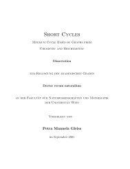
Figure 1.1: From top left: CRNs occur in combinatorial chemistry, atmospheric
processes, combustion, and metabolic networks.

levels of metabolites (regulation) or may be influenced by external factors
(control). Control analysis [58] and thermodynamic analysis of flows [79]
provides a measure for the influence of a single reaction on the fluxes in
the whole CRN. The related flux analysis [35, 21] defines for that purpose
the flux coefficient, and, for the dependence on substrate or external concentrations,
elasticities and response factors, respectively. Further analysis
then yields steady states, and further structural analysis reveals constant elements
(maximal conserved moieties), conservation relations and elementary
modes of a CRN. Maximal conserved moieties are elements of species common
to a group of species, remaining unchanged as the species transform into
another. Conservation relations are linear combinations of species concentrations
that are constant in time. Finally, elementary modes are parts of a
CRN whose fluxes can be isolated independently. They are especially interesting
for biotechnological applications aiming to increase these fluxes [106],
and for understanding evolutionary optimization of metabolic networks [58].
The preceding paragraph showed how to analyze CRNs, i.e. how to extract
information from a given CRN. But just as CRNs can be analyzed, they can
also be synthesized. In this case CRNs are built from scratch or simulated
in silico. The way a network develops may be observable by building it
from minimal premises, and even afford predictions. On the other hand,
a simulation is valuable as a substitute for potentially more complicated
experimental studies. In ch. 2, a survey of CRN “synthesis” describes this
research area.
Due to the diversity of CRNs, it is of immediate interest to determine
which structural features are generic properties of large-scale reaction networks
and which properties are the consequence of a particular chemistry.
The graph-theoretic study of the structure of CRNs has been started by Balandin
[9] and has been continued by the research on the enumeration and
classification of CRNs [110].
The study of generic properties of CRNs is more recent and has identified
many small-world networks among them [118, 1, 55]. This means that the
graphs spanned by these networks have only short paths between any of their
nodes. This observation would be made more meaningful by comparison with
a generic CRN. It could be investigated if any random CRN and not only
a specific network has small-world properties. Other interesting properties
would be the scaling behavior, the network diameter, or the network center,
for example.
The goal of this thesis is to model chemical reactions networks. The model
should simulate how molecules of different constitutions, that determine their
reactivity, are combined to a network of interconnected reactions. Eventually,
we are interested in generic properties of a chemical reaction network by
3

4 CHAPTER 1. INTRODUCTION
¡ ¡ ¡
¢ ¢
¡ £ ¡
¢
¡ ¡ ¡
Figure 1.2: Alexander Crum Brown’s master’s thesis [14, 69] was the first scientific
publication to use systematically the graph representation of molecules
in today’s form.
unbiased construction.
There are many models simulating different parts of CRNs at different
accuracy levels (see sect. 2). The present Toy Model could be situated on a
medium level of abstraction. QM/MM simulations, which use 3D information,
are chemically more accurate, but may suffer from high time complexity.
On the other hand, very abstract artificial chemistries are useful to study the
evolution of networks but, like the λ-calculus (sect. 2.1), do not include thermodynamics
or other important features of chemistry.
In chemistry, the changes of molecules upon interaction are not limited
to quantitative properties of physical state, such as free energy or density,
because molecular interactions do not only produce more of what is already
there. Rather, novel molecules can be generated. This is the principal difficulty
for any theoretical treatment of the situation. Chemical combinatorics
makes it impossible to think of molecules as atomic names whose reactive relationships
are tabulated. A computational approach to large scale reaction
networks therefore requires an underlying model of an artificial chemistry to
capture the unlimited potential of chemical combinatorics. The investigation
of generic properties of chemistries requires the possibility to vary the
chemistry itself; hence a self-consistent albeit simplified combinatorial model
seems to be more useful than a knowledge-based implementation of the real
chemistry which inevitably is subject to sampling biases.
We are going to use a graphical representation of molecules in connection
with a simple quantum mechanical wave function analysis. The analysis determines
the reactions and dynamics of CRN. This Toy Model of chemistry
is computationally inexpensive and still retains the “look and feel” of the
real (detailed quantum-mechanical) thing. In the following, the Toy Model
is briefly described.
The representation of molecules as graphs has been used by chemists
since the nineteenth century (fig. 1.2). In textbooks and scientific publica-

5
−→
C C A
A C
C
G
P
G T
A
U
C CACAG U
G
U
C C U G
G
G C U U A A A
G C G G A U U G G
UA
G C GC U
C C A U
A Y G AC
C G
A A
U A
U G
C G
A
G A
D G G
D G
O
−→
NH 2
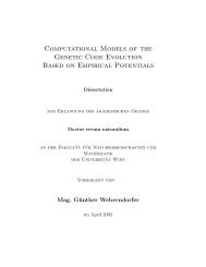
Figure 1.3: Analogy between the reduction of a RNA structure to its secondary
structure (top, tRNA) and the reduction of a molecule to its graph
representation (bottom, propenamide).
tions, the natural way for a chemist to describe a molecule is a graph. The
nodes of graph are the atoms and the edges are the bonds. The graph reflects
and was the first to explain the phenomenon of constitutional isomery [14].
Indeed, the description of molecular structures is one of the roots of graph
theory [17, 108]. However, molecules can also be viewed as an agglomeration
of atoms or nuclei in three-dimensional space. Most computational chemistry
software packages implement molecules as a list of nuclei or atoms with
three-dimensional coordinates. The position of the electrons, i.e. the electron
distribution is then calculated as a charged cloud floating between the nuclei.
Nevertheless, it can be argued that in the graph representation, the edges or
bonds are already an educated guess on the electron distribution. Thus the
loss of steric information in the graph representation might not be as radical.
The reduction of a three-dimensional molecule to the topology of its graph
is somewhat analogous to the secondary structure model of RNA (fig. 1.3).
The latter is also a reduction of the complete quaternary three-dimensional
molecular structure to a tree representation. Three-dimensional coordinates

6 CHAPTER 1. INTRODUCTION
and symmetries are ignored. It nevertheless leads to excellent qualitative
predictions of thermodynamic properties [61].
The graph representation of the molecule is now combined with a simple
energy calculation. This suffices to fulfill the requirements of the laws
of mass and energy conservation. It is then straightforward to represent reactions
by graph rewritings (see ch. 2 and 4). The graph rewriting rules
correponds to the reaction mechanism as understood by chemists. The Cannizarro
reaction [16], for example, takes place between two aldehydes and
produces an acid and an alcohol by disproportionation. The graph rewriting
rule is analogous and adds a solvent proton node and a hydride node to
one aldehyde graph to form an alcohol graph. The second aldehyde graph
looses the former hydride node and gains a hydroxyl group (formed by two
nodes), thus yielding the acid. The advantage of this reaction representation
is that it represents the reaction itself also by graphs, and thus does not have
the inherent limitations of e.g. string representations. It is also, of course,
more flexible and simpler than a hard-coded implementation of reactions as
complicated reactions might be very time-consuming to encode one per one.

Chapter 2
Artificial Chemistries
In this section we very briefly survey artificial chemistry models. Tab. 2.1
compares different CRN models based on their implementation of the three
components molecules, reactions and networks [26]. The models can also be
categorized according to abstraction level and intended application. Very abstract
models simulate artificial chemistries in which string or logical elements
interact, like in the λ-calculus. There networks are built in a bottom-up approach
to be studied phenomenologically. On the other hand, models for
practical applications tend to be top-down. They concentrate on describing
interactions and try to predict, for example, the time or space evolution of
concentrations. Some approaches are further described in the following.
2.1 The λ-calculus
The λ-calculus is a proof theory of constructive logic. This area of logic
studies proofs using the interaction of logical elements called λ terms. Every
λ term may be applied to another λ term to generate further λ terms, i.e. the
deductions. Thus λ terms can be interpreted as objects as well as functions.
The λ-calculus studies those functions and their applicative behavior, and
indeed was founded to develop a general theory of functions, providing a
foundation for logic and parts of mathematics [20]. In the related field of
computer science, Turing [112] showed that the λ-calculus is strong enough
to describe all mechanically computable functions. Ref. [109] reviews models
based on the λ-calculus.
In analogy to λ terms, molecules in chemistry can be viewed both as
undergoing and fueling a reaction, i.e. reactants and reagents. This analogy
was exploited in the base model of [40]. We will describe now features of
this model. It consists of a well-stirred flow reactor of interacting functions
7

8 CHAPTER 2. ARTIFICIAL CHEMISTRIES
Table 2.1: Comparison of different CRN models.
Molecules have: Reactions are: Dynamics are:
Model Topo- 3D coor- Rewrite QM/ Exhaustive Explicit
logy dinates rules MM generation collision
Toy Model • • •
Atomoid [130] • • •
EROS [50] • •
Patel [83] • • •
GoForth [129] • • •
CCM [68] • • •
Faulon [33] • •
λ-calculus [40] • •
Polymer AC [8] • • •
String AC [27] • • •
Lancet [75] • •
ARMS [107] • • •
Automata • •
[66, 91, 128]
A
{ }} { { }} {
( λx.((x)λy.y)x) λu.(u)λv.v →
normalization/reaction completion
{ }} {
((λu.(u)λv.v)λy.y)λu.(u)λv.v → ((λy.y)λv.v)λu.(u)λv.v → (λv.v)λu.(u)λv.v →
λu.(u)λv.v
} {{ }
“product”
B
Figure 2.1: Example reaction triggered off by applying λ term A onto λ term
B (after [42]). (A)B denotes an application, and x, y, u, and v are “atomic
names”. λx.A means that the λ term A is a function of x.
in the frame of the λ-calculus. λ terms are interpreted as molecules and
interactions as chemical reactions. An interaction or deduction is carried out
by a rewrite rule on the λ term. A non rewritable λ term is called a normal
form and is equivalent to a stable molecule (fig. 2.1).
The λ-calculus can also be viewed as a formal theory of chemistry. Its
advantage as an artificial chemistry is that it handles changes in the structure
of an object, and that, moreover, the behavior of its objects depends on

2.2. ATOMOIDS, GRAPHS, AND MATRICES 9
their structure. Quantum mechanics also uses formal laws, but its consideration
of molecules is too minute for an analysis of a CRN. The λ-calculus
makes CRNs and the laws of their dynamics more transparent by using less
detail. For example, CRNs or organizations of molecules do evolve in the
λ-calculus. There is emergence of self-maintaining sets of functions, with
a specific grammar defining their syntax, acting in accordance to invariant
algebraic laws. They define a closure of interaction. In ref. [41], ecologies of
different complexity levels are built.
Nevertheless, it is difficult to build a chemically sensible model of molecular
decay in the λ-calculus. The model of [40] defines functions with finite
lifetime, but in chemistry, the lifetime of molecules is understood to be determined
by their reactivity and thus their structure. Although the Toy
Model inherits the concept of rewriting from [40], it lets molecules decay
based on their structure. Furthermore, the problem of molecular decay in
the λ-calculus leads to violation of the law of mass conversation, and so does
the lack of an equivalent of the chemical atom. A normalization, equivalent
to reaction completion [42], shortens the λ term, and it is difficult to find
a function that is preserved during a reaction, as an atom would be. Selective
reactivity, multiple products, and rate constants, i.e. thermodynamics,
also remain to be implemented into the calculus [42]. Terms in the lambdacalculus
may always react and thus can build a chemical perpetuum mobile.
The Toy Model addresses those issues and follows the simple bottom-up approach
of the λ-calculus: simple data structures can be applied onto each
other and may evolve into a complicated chemistry. In addition, the graph
representation of molecules and a judicious choice of graph rewritings ensures
mass conservation. Reactions can be encoded in graph rewritings in which
the number and and mass of atoms and thus the total reactant mass does
not change in the course of the reaction.
2.2 Atomoids, graphs, and matrices
The Atomoid model of [130] is inspired by the work of L. S. Penrose on
self-reproducing mechanical models. It uses the graph representation for
molecules, which are built from atoms connected by bonding hands. Bonding
hands differ by energy level and energy structure. For a reaction to happen, it
suffices that the connection of bond handles leads to an increase of energy of
the bond handles. The reaction changes the atomic structure and the energy
structure, which in turn changes the energy and may lead to the rupture of a
distinct bond in the newly formed molecule. Bond handles may also interact
via the exchange of photons. The photons are needed to avoid a freezing of

10 CHAPTER 2. ARTIFICIAL CHEMISTRIES
Educts Intermediates Products
Figure 2.2: The Atomoid model. Molecules are built from “atoms” connected
by bond handles differingin energy level and energy structure.
Initiation
−→
Elongation
−→
Termination
−→
Figure 2.3: Simulation steps of RNA growth by the rewritable graph chemistry
of [78].
the system from the start. These simple artificial atomic reaction rules lead
to dissipative structures. The model enables one to follow on an atomic level
how those dissipative structures lead to the emergence of self-reproductive
hypercycles. Fig. 2.2 shows a simple example network.
The rewritable graph chemistry of [78], fig. 2.3, is designed to be
complementary to the string-oriented analysis of nucleic acid polymers. The
string editing is replaced by graph rewriting rules. They are encoded by
subgraph graph replacements on labeled graphs called variable graphs, rep-

2.2. ATOMOIDS, GRAPHS, AND MATRICES 11
Mass spectrum
calculation
Molecular
property
prediction
EROS
ODE integration
reactors, phases
and modes
Reaction rules
Figure 2.4: Modular organization of the organic chemistry simulation package
EROS.
resenting chemical reactions. This model is used to simulate DNA and RNA
transformations like enzymatic processing or combinatorial networks of catalyzed
reactions. The model generates all possible derivation paths. It could
be applied also to small organic molecules.
The Iterated Graph Model of [83] applies a limited subset of chemical
reactions to a soup of molecules. Each chemical reaction, in this case
food-browning reaction, is implemented as a separate function working on a
molecular graph. The dynamics of the system are simulated by explicit collision.
Pairs of molecules are chosen with a frequency proportional to their
concentration in the soup and are submitted to a reaction function with a
probability equivalent to the reaction rate. The reaction rates are fitted to
match the evolution of the concentrations to experimental values.
EROS [50] is similar to the Toy Model by its straightforward implementation.
Its basic architecture transparently reflects the three components
molecules, reactions, and networks. The energy calculation for molecules
involves are rule-based efficient generation of 3D coordinates, which makes
it possible to accurately calculate many molecular properties. Reactions are
hard-coded by two general reaction schemes. They are essentially pseudopericyclic
σ and π electron shiftings whereby bonds are broken and formed.
The CRN is generated exhaustively. The CRN generation can be combined
with a “sifting-out of reactions”, a model reduction based on reaction site
properties, reaction enthalpy and reaction rates. EROS also implements
phases, see fig. 2.4 for its module-oriented organization.
Approaches trying to avoid hard-coding reactions need to use a description
of generic reactions [59]. The description used by the Toy Model is
presented in sect. 4.1.
SMIRKS is a development of SMILES (sect. 3.3) capable of encoding
generic reaction transforms as a line notation. However, rewrite rules are
graphs and thus do not have the limitations of a line notation representation.
Although all graph representations of generic reaction contain the same
information [110, ch. 1], they differ by the stage or the part of the reaction

12 CHAPTER 2. ARTIFICIAL CHEMISTRIES
that is described. The imaginary transition structure [45] merges constant
and changing parts into a single representation, while the skeleton of transformation
[95] shows only the changing parts.
[83, 88] uses a hybrid approach with the Reaction Description Language.
This language encodes the steps of reaction site identification, reaction matching,
and reactant manipulation. The code is compiled and yields a hardcoded
function for each reaction.
I. Ugi and coworkers [113, 114] have developed a a formal theory of chemical
reactions called the Dugundji-Ugi-model. In this model, reactions are
interconversions between isomers of ’ensembles of molecules’ (EM). The concept
of stoichiometric transformation in this model is used in the reaction
simulation part of the Toy Model (see sect. 4.1). EM and reactions can be
represented as matrices BE and R, such that the reaction R from BE 1 to
BE 2 is equivalent to writing BE 2 = BE 1 + R. The off-diagonal entries of
BE are bond orders between atoms, diagonal entries are number of valence
electrons in lone pairs. Reaction generators (RG) may generate all R from
a given BE 1 (RGB) or all BE from a given R (RGR). The program IGOR
[39] is an RGR and generates new organic reactions and reaction networks
between known educts and products. Koča et al. have developed an extension
of the DU-Model, the synthon model [60, 73]. Here, lone electron pairs
are represented by loops.
[33, 43] review methods to reduce the combinatorial explosion of possible
reactions in formal models of CRNs. Reduction may be choosing a subset of
reaction through an educated guess or in accordance to experimental observation.
This subset may be a certain class of reaction, thus representing a
special chemistry, or it may be formed by picking one representative reaction
for each class of reactions. Finally, the subset used by [33] includes reactions
according to their contribution to the reaction dynamics, by their concentration
or by their rate constant. Thus the reaction mechanism reduction is
achieved simultaneously with the CRN generation.

14 CHAPTER 3. MOLECULES
Schrödinger equation
ĤΨ = EΨ
⇑
⇓
Born-Oppenheimer
LCAO and Extended Hückel
VSEPR and Tight Binding
Generalized Eigenvalue Problem
⎛
⎞ ⎛
⎞
. .. . ..
⎜
⎟ ⎜
⎟
⎝ H AOi −AO j ⎠C = ⎝ S AOi −AO j ⎠CE
. .. . ..
Figure 3.1: Schematic derivation of the used electronic calculation method.
H AOi −AO i
, S AOi −AO j
and K are given parameters (see equations 3.13).
the Schrödinger equation is separated into a part describing the electronic
wave function Ψ el for fixed nuclei,
Ĥ el Ψ el = E el Ψ el , (3.3)
and a part describing the nuclear wave function. The electronic Hamilton
operator is:
(
)
∑e −
Ĥ el = − 1 2 ˆ∇
∑nuc
2 Z I
∑e − ∑e − 1 ∑nuc
∑nuc
Z I Z J
i −
+ , (3.4)
r
i
I iI r
i j>i ij r
} {{ } }{{} I J>I IJ
} {{ }
ĝ ij V n
ĥ i
+
where ˆ∇ is the nabla operator, Z i is the nuclear charge of the atom i and r ij

3.1. EXTENDED HÜCKEL THEORY 15
is the distance between the nuclei or electrons i and j. e − and nuc indicate
sums running over all electrons and nuclei, respectively. V n , the electrostatic
nuclear repulsion, does not depend on electron coordinates and is thus an
additive constant to the final energy. For more clarity, it is omitted from the
following equations.
Hartree proposed the orbital approximation, in which the wave function
is built from Slater determinants,
∣ ∣∣∣∣∣∣∣∣ φ 1 (1) φ 2 (1) · · · φ N (1)
Ψ SD = √ 1 φ 1 (2) φ 2 (2) · · · φ N (2)
. N! . . .. . (3.5)
.
φ 1 (N) φ 2 (N) · · · φ N (N) ∣
The φ are one-electron wave functions, called molecular orbitals (MO) or
spin orbitals. The energy of a single Slater determinant will be used lateron
for the variational principle. It may be written as
∫
E el = Ψ SD Ĥ el Ψ SD d τ (3.6)
and decomposed into one-electron or core integrals ∫ φ i (i)ĥiφ i (i) dτ, twoelectron
Coulomb integrals ∫ φ i (i)φ j (j)ĝ ij φ i (i)φ j (j) dτ, and two-electron exchange
integrals ∫ φ i (i)φ j (j)ĝ ij φ j (i)φ i (j) dτ.
Semi-empirical methods, Extended Hückel Theory [62, 65] for instance,
now further approximate the wave function by building it from one
single Slater determinant, thus neglecting electron correlation.
First, using the basis set or LCAO approximation, each φ is expanded
as a linear combination of atomic orbitals χ (LCAO) :
φ i = ∑ j
C ij χ j . (3.7)
The definition of the electron density ρ in LCAO will be needed in sect. 3.4
and will be shortly presented here. The electron density or the probability
of finding an electron in a MO φ i , occupied by n i electrons, at the position
defined by the position vector r is
ρ i (r) = n i φ 2 i (r) . (3.8)

16 CHAPTER 3. MOLECULES
As the MO s are normalized, we have:
∫
∫
ρ i (r)dr = n i φ 2 i (r)dr = n i .
Thus
∫
∑
∫
ρ i (r)dr = n i C ji C ki χ j χ k dr
⇒
j,k∈AO
∑
j,k∈AO
C ji C ki S jk = 1 . (3.9)
Now, neglecting electron-electron repulsion ĝ ij , the Hamilton operator is
approximated as a sum of one-electron operators:
Ĥ = ∑ i
ĥ i . (3.10)
This gives the total energy as a sum over the one-electron energies of occupied
molecular orbitals. Using the variational principle, which states that the best
molecular orbitals are those that minimize the energy, we obtain a generalized
eigenvalue problem:
HC = SCE, (3.11)
where C is the matrix of the LCAO coefficients in eq. 3.7, E is the diagonal
matrix of one-electron energies, and
∫
H ij = χ i Ĥχ j dτ
∫
(3.12)
S ij = χ i χ j dτ .
Finally, the H ij are parametrized:
H ii = −I i
(
Ii + I j
H ij = −κ
2
)
S ij ,
(3.13)
in terms of the overlap integrals S ij , the Wolfsberg-Helmholtz constant κ,
and the atomic valence state ionization potentials I i .
Theories related to Extended Hückel theory have been reviewed in [103].
Hückel-type calculations were first applied to saturated systems by [100].

3.2. FURTHER APPROXIMATIONS 17
K. Fukui used a LCAO approach with hybridized valence orbitals (LCVO)
and calculated energies, charge distributions and dipole moments. He used
perturbation theory to develop from there the Frontier Molecular Orbital
Theory (see sect. 3.6) and to calculate reactivities. Further refinements
of EHT were made to account for electron-electron interaction. An iterative
EHT (IEHC) was developed in order to obtain more accurate atomic
charges. Electron-electron correlation is usually completely neglected but
has been approximated by Atom Superposition and Electron Delocalization
Molecular Orbital theory (ASED-MO) [4, 5], thus affording better prediction
of geometries.
3.2 Further approximations
The basis set used for the LCAO is the 1s orbital for hydrogen and hybrid
AOs for carbon, nitrogen and oxygen. Hybrid AOs are linear combinations of
Slater-type orbitals, coefficients depending on the hybridization of the atom.
Tab. 3.1 shows the definition of Slater-type and hybridized orbitals used.
Sulfur and phosphor would also require d-orbitals and their hybrids dsp 3 and
d 2 sp 3 .
Hybrid orbitals are used because we can assume for simplicity that they
are always oriented along bonds, such that for given atom types and hybridizations,
there is always the same overlap. Thus, the corresponding
overlap integral, instead of being calculated repeatedly, can be replaced by
a constant parameter, in analogy to the Tight Binding approximation for
solids [104]. This would not be the case for normal Slater-type orbitals.
A molecule is therefore completely determined by a vertex labeled graph
g, which was introduced by O. Polanski [87]. A graph g = (V, E) is a set of
vertices V and a set of edges E. Vertices are elements v i . Edges are pairs
of vertices (u, v) ∈ V × V defining connected vertices. The vertices of g are
the atom orbitals (labeled by atom type and hybridization); edges denote
overlaps of orbital on adjacent atoms. This orbital graph g is obtained in
an unambiguous way from the chemical structure formula by means of the
rules described in the following. It follows that, in the framework of the Toy
Model, the structure formula already encapsulates the complete information
about the molecule.
The rules for constructing the orbital graph are:
• Overlaps are only non-zero (orbital graph edges exist only) between
orbitals on connected atoms.
• Only the overlaps shown in figs. 3.4, (a) and (b) (direct σ, semi-direct),

18 CHAPTER 3. MOLECULES
Table 3.1: Definition of Slater-type (STO), sp 3 -, sp 2 - and sp-hybridized
atomic orbitals. STOs are electron distributions, given here in spherical coordinates
(r, θ, φ). Y l,m are the usual spherical harmonic functions and n, l, m
define the orbital type. N is a normalization constant and ζ is a parameter,
both varying with n, l, m and Z, the atomic number.
χ ζ,n,l,m (r, θ, φ) = NY l,m (θ, φ)r n−1 e −ζr
(general form)
STOs
1s = Ne −ζr
2s = N(1 − ζr)e −ζr
2p x = Nζre −ζr cosθ
= Nζre −ζr sin θe ±iφ
2p y,z
χ 1 = 1 2 (2s + 2p x + 2p y + 2p z )
sp 3 orbitals
χ 2 = 1 2 (2s + 2p x − 2p y − 2p z )
χ 3 = 1 2 (2s − 2p x − 2p y + 2p z )
χ 4 = 1 2 (2s − 2p x + 2p y − 2p z )
χ 1 =
√
1
3 2s + √
2
3 2p x
sp 2 orbitals
χ 2 =
χ 3 =
√ √ √
1 1 1
3 2s − 6 2p x +
2 2p y
√ √ √
1 1 1
3 2s − 6 2p x −
2 2p y
χ 4
= 2p z
χ 1 = 1 √
2
(2s + 2p x )
sp orbitals
χ 2 = 1 √
2
(2s − 2p x )
χ 3
= 2p y
χ 4
= 2p z

3.2. FURTHER APPROXIMATIONS 19
Figure 3.2: π-overlap between p orbitals.
3.2, and 3.3 (π, hyperconjugation and fictitious) are implemented. The
other possible overlaps between hybridized orbitals, see fig. 3.4, (c) and
(d) (indirect), are set to zero as they are in average as low as 0.1 .
• In the style of [89] and [86, ch. 6.4], the term hyperconjugation is used
for overlaps between a p orbital and a neighboring, but “indirect” oriented
sp 3 orbital. Only one of the three sp 3 is randomly chosen for an
overlap proportional to the π overlap of the corresponding atoms. The
other two “indirect” oriented overlaps are set to zero. In order to avoid
choosing randomly an orbital, but to keep the σ-MOs and the π-system
coupled, a second factor is defined for the overlap between the p orbital
and the “direct” oriented sp 3 orbital. This factor may be used instead
of the hyperconjugation factor. The overlap is dubbed “fictitious”.
• The set of overlaps is determined by the hybridization of the two atoms
involved in the bond. Tab. 3.2 shows all the possible combinations of
hybridizations and ensuing overlaps. The set of overlaps only depends
on the type and orientation of the orbitals.
Thus the energy calculation in the Toy Model is parametrized in terms
Table 3.2: Sets of overlaps depending of hybridization on bonding atoms.
number of overlaps
Hybridization of (see figs. 3.2, 3.3 and 3.4)
atom 1 atom 2 σ semi. π hyper. fictitious
sp 3 1 6 0 0 0
sp 3 sp 2 1 5 0 1 1
sp 1 4 0 1 1
sp 2 sp 2 1 4 1 0 0
sp 1 3 1 0 0
sp sp 1 2 2 0 0

20 CHAPTER 3. MOLECULES
Figure 3.3: Hyperconjugation and artificial overlap between p and sp 3 orbitals.
a b c d
Figure 3.4: Overlap along a bond (a), “semi-direct” overlap, where only one
of the orbitals is directed along the bond (b), and the two possibilities of
“indirect” overlaps of two sp 2 orbitals at adjacent atoms (c,d). In the graphtheoretical
model (c) and (d) are equivalent because the orientation in the
plane is not a property of the molecular graph. In the case of a symmetric
molecule, randomly assigning (c) and (d) could break the symmetry of the
molecule, and moreover difficult to reproduce. In the current implementation
“indirect” overlaps are neglected.
of ionization energies I j and overlap integrals S ij of the usual Slater-type
hybrid orbitals. The numerical values are listed in appendix A. The S ij for
direct overlaps are given explicitly in the appendix, the other overlaps are
parametrized using simple scaling factors applied on the direct overlaps, see
tab. 3.2. The factor used to calculate the semi-direct overlap from the direct
overlaps depends on whether one of the bonded atoms is a hydrogen.
Calculations (see appendix A) show that the approximation by this scaling
factor is inaccurate. However, it is kept for simplicity, but might be later
replaced by an independent set of parameters.
The overlaps over bonds which lie in three- and four-membered rings

3.2. FURTHER APPROXIMATIONS 21
are also scaled by factors. This reflects the weakness of “banana-bonds” in
constrained rings. The factor 3-ring applies to all bonds in a three-membered
ring. The factor 4-ring applies only to other bonds in four-membered rings,
in order to reflect that bridging bonds, i.e. bonds contained in two rings, are
as strained as bonds in three-membered rings (more precise data is available
from [11]).
The hybridization of a particular atom is determined using valence-shell
electron pair repulsion (VSEPR) theory [53]. VSEPR is a simple method to
predict the geometry of compounds. The only thing needed is the connectivity
of the compounds, which is given by definition by the graph representation
of the molecule. The VSEPR theory assumes that the valence-shell electron
pairs of any atom in the molecule are arranged in a fashion that minimizes
electrostatic repulsion. Electron pairs are represented by the bonds, i.e. edges
of the molecular graph, and by lone electron pairs, whose number depends
only on what element the atom is. Every bond, be it simple, double or triple,
counts as one electron pair. The geometry of atoms depends in the end on
the number of electron pairs, in bonds and in lone pairs. A total of 2 leads
to linear geometry and sp hybridization, 3 to trigonal geometry and sp 2 hybridization,
and 4 to tetrahedral geometry and sp 3 hybridization. The atom
on which VSEPR is applied is called the central atom. Tab. 3.4 summarizes
the results and gives examples for neutral atoms and a charged central atom.
To account for resonance structures, a few more rules are added. Resonance
structures occur when more than one Lewis structure can be drawn
for a molecule. The most common situations are adjacent π bonds, and a
lone pair adjacent to a π bond [86, sect. 6.3]. The former has been taken
care of by always establishing π interactions between adjacent sp 2 atoms (see
tab. 3.2). The latter corresponds to the situation where, when drawing alternative
Lewis structures, lone pairs and π bonds are converted into each
other. In fact, the electrons are delocalized.
Thus the hybridization of an atom with lone pairs depends on its neighbors,
namely those who are not sp 3 hybridized. The current implementation
Table 3.3: Scaling factors for calculating remaining overlaps from the overlaps
in Tab. A.2
indirect hyper- banana
all H conjugation symmetric 3-ring 4-ring
0.1 0.0 0.8 0.0 0.7 0.8

22 CHAPTER 3. MOLECULES
Table 3.4: Geometry of C, N and O according to VSEPR theory.
Number of e − in
Atom lone Hybridization
bonds pairs total
4 0 4 sp 3
C 3 0 3 sp 2
2 0 2 sp
3 1 4 sp 3
N 2 1 3 sp 2
1 1 2 sp
O
2 2 4 sp 3
1 2 3 sp 2
O − 1 3 4 sp 3
Table 3.5: Resonance.
hybridization # of lone pairs change in
of connected on central hybridization
atom atom of central atom
1 sp 3 → sp
sp 2 2
2 sp 3 → sp 2
sp
1
2
sp 3 → sp 2
sp 2 → sp
sp 3 → sp
sp 2 → sp
starts from the latter atoms (central atom) and then looks for atoms with
lone pairs which are connected over single bonds. The changes in hybridization
resulting from resonance implemented in the Toy Model are shown in
tab. 3.5.
The orbital graph resulting for propenamide is shown in fig. 3.5.
By the preceding method, the orbital graph and thus H and S are completely
determined by the original chemical graph. It contains only information
on atom types and connectivity, but this suffices to derive hybridizations
and overlaps according to VSEPR. Per definition, any property may now be
calculated for the molecule from its wave function (see sect. 3.4).

3.3. CHEMICAL STRUCTURE REPRESENTATION 23
H
1s
H
1s
H
1s
2sp 2 2sp 2
C
2sp 2 p
1s
H
2sp 2
C
2sp 2
N
2sp 2 2sp 2 2sp 2
2sp 2
2sp 2 2sp 2
p
p
2sp 2 2sp 2
C
2sp 2 p
2sp 2
O
p
1s
H
Figure 3.5: Orbital graph of propenamide H 2 C = CH − C(= O) − NH 2 . Direct,
semi-direct σ-overlaps, and π-overlaps are represented by solid black,
dashed, and solid gray lines.
3.3 Chemical structure representation
As the Toy Model only needs to store a graph to represent a molecule completely,
an appropriate structure representation format has to be selected.
A particularly convenient encoding is the Graph Meta Language (GML)
[90]. It is a simple and flexible file format for graphs, designed to represent
arbitrary data types as ASCII files. The BNF notation for GML is:
GML ::= List
List ::= (whitespace* Key whitespace+ Value)*
Value ::= Integer | Real | String | [ List ]
Key ::= [ ’a’-’z’ ’A’-’Z’ ] [ ’a’-’z’ ’A’-’Z’ ’0’-’9’ ]*
Integer ::= sign digit+
Real ::= sign digit* . digit* mantissa
String ::= ’"’ instring ’"’
sign ::= empty | + | -

24 CHAPTER 3. MOLECULES
digit ::= [’0’-’9’]
Mantissa ::= empty | ’E’ sign digit
instring ::= ASCII - {\&,"} | \& character+ ;
whitespace ::= space | tabulator | newline
Here, graphs are encoded by blocks starting with the keyword graph.
Inside this block, nodes and edges are defined by key-value list using the
keywords node and edge. The following example shows how their attributes
are defined:
# Isobutane
graph [
node [ id 1 label "C" ]
node [ id 2 label "C" ]
node [ id 3 label "C" ]
node [ id 4 label "C" ]
]
edge [ source 1 target 2 label "-" ]
edge [ source 1 target 3 label "-" ]
edge [ source 1 target 4 label "-" ]
Labels of atoms and bonds define their type, i.e. C, N, or O for atoms,
and − (single), = (double), or # (triple) for bonds.
The GML format is precise and non-redundant, but long and tiresome to
read. Thus, a different format is need for quickly displaying lists of molecules.
SMILES (Simplified Molecular Input Line Entry Specification) 1 is a line
notation, i.e. a string representation for molecules. SMILES are compact and
their grammar is easy to learn. Their similarity to structural formulae makes
their grammar intuitive for chemists.
Moreover, in order to eliminate duplicates from a list of molecules or to
subtract one list of molecules from another, as in sect. 5.1, a comparison
of the structural formulae must be performed. This amounts to a test of
graph isomorphism, for which neither an efficient algorithm nor proof of NPcompleteness
is known in general [72]. The chemically relevant problem of
testing graph isomorphism with bounded vertex degree (bounded valency of
the atoms), however, can be solved in polynomial time [77]. We transform
the molecular graphs into their canonical SMILES representation [120, 121].
The isomorphism test then reduces to simple string comparison.
1 from http://www.daylight.com/smiles/f smiles.html: “SMILES originated in
the depths of the US government, where humorous names for things are frowned upon
unless they are acronyms.”

3.3. CHEMICAL STRUCTURE REPRESENTATION 25
CH 4
C
or C(H)(H)(H)H
H 3
C CH 3
CC
or C(H)(H)(H)C(H)(H)(H)
CC(C)C or C(H)(H)(H)C(H)(C(H)(H)(H))C(H)(H)(H)
OH
OC(C = C1) = CC = C1 or HOC(C(H) = C1H) = C(H)C(H) = C1H
Figure 3.6: An extremely brief SMILES tutorial.
The BNF notation of the subset of SMILES used in the Toy Model is:
atom ::=
’C’ | ’N’ | ’O’ | ’H’
bond ::= | ’-’ | ’=’ | ’#’
chain ::=
|
branch ::= ’(’ ’)’
| ’(’ ’)’
| ’(’ ’)’
| ’(’ ’)’
smiles ::=
|
In addition to these rules, which describe trees, cycles are indicated by
adding identical digits to the atoms closing a cycle. Hydrogen atoms may be
included implicitly or explicitly. See fig. 3.6 for a quick list of examples.
The canonical SMILES are built using rules described in [121]. First a
graph data structure with canonical labeling and ranking is built, ordered
according to the labels and ranks. Then a unique SMILES is generated,

26 CHAPTER 3. MOLECULES
whereby branching decisions in the SMILES tree rely again on the ranking
and labeling.
A SMILES uniquetizer is available fromoutreach@superior.dul.epa.gov
and http://www.epa.gov/med/databases/smiles.html. It transforms
SMILES into unique SMILES (USMILES) such that two identical molecules,
i.e. with isomorphic graphs, have the same USMILES. The USMILES may
serve as a unique identifier, which is needed for the CRN generation (ch. 5).
By using USMILES, the graph isomorphism test reduces to a simple string
comparison.
A number of other distinct representations of (organic) molecules are used
in different programs:
• IUPAC Nomenclature is in principle able to give a unique representation
of a molecule. IUPAC-names are, however, rather uncomfortable
to parse.
Heptacyclo[7.5.1.0 2,14 .0 5,12 .0 5,15 .0 8,10 .0 11,13 ]pentadecane
• WLN WISSWESSER LINE NOTATION [116] is based on an
aggregate representation of the molecule in which symbols represent
entire functional groups.
Example: QVYZ1RDQ is the code for
(OH−)(−CO−)(−HCNH 2 −)(−CH 2 −)(−C 6 H 5 )(para)(−OH), i.e.:
HO
NH 2
OH
O
• Registry Numbers. Every new organic compound gets an arbitrary
number in Chemical Abstracts (CAS) or Beilstein (CCID). Clearly,
this representation is not useful for the purpose of generating reaction
networks.
• Fragmentation Codes. The two main systems are GREMAS (Genealogische
Recherche mit Magnetband-Speicherung) [12, 44] and the

3.4. WAVE FUNCTION ANALYSIS 27
Derwent Fragmentation Codes, which are often used in patent search
systems. The idea is to subdivide the structure into fragments that are
then represented by three-letter codes of the form Genus / Species /
Subspecies, e.g. EAD = Alcohol/free alcohol/free aromatic alcohol.
This systems is rather complicated, hard to adapt to new chemistries,
and very hard if not impossible to convert into a canonical representation.
• Connection Tables. A molecule is represented as a list of atoms and a
list of bonds connecting these atoms. There is a plethora of file formats.
MOL and SDF Files are simple flat format files, and the most used ones,
see http://www.mdli.com/downloads/literature/ctfile.pdf.
3.4 Wave function analysis
The generalized eigenvalue problem can be transformed into a standard (symmetric)
eigenvalue problem using a congruence transformation by factorizing
the metric, here overlap matrix [124, sect. 1.31, 5.71]. Because the basis set
is orthogonalized, the transformation is called orthogonalization.
In the Toy Model, Löwdin’s symmetric orthogonalization with S = S 1/2 S 1/2
is used. S is assumed to be positive-definite (it should be noted that too big
overlaps (> 0.8) may lead to a non-positive-definite overlap matrix). Eq. 3.11
then transforms to the symmetric form:
(S −1/2 HS −1/2 )C ′ = C ′ E, (3.14)
where C ′ = S 1/2 C.
Using this method, the overlap matrix stays exactly symmetric and fewer
numerical errors than in the canonical method are introduced. In canonical
orthogonalization, a Cholesky decomposition S = LL T is used. This method
is more efficient than the calculation of S −1/2 but more error-prone. Numerical
errors may also break the symmetry of a molecule. However, there are
further developments leading to linear scaling algorithms for those matrix
computations [19].
The total electronic energy of the molecule is obtained by the formula
E = ∑ i
n i E i , (3.15)
where n i is the occupation number of the MO φ i .
The electron distribution is derived from eq. 3.9 by using a partitioning,
e.g. isolating one summand for each atom. The only way of identifying in the

28 CHAPTER 3. MOLECULES
Toy Model to which atom an electron belongs is by the AOs. Furthermore,
as Löwdin’s method was used for the orthogonalization, it is straightforward
to use Löwdin partitioning for population analysis. This is equivalent to
performing the partitioning in the orthogonalized basis χ ′ = S 1/2 χ, where
S ′ jk = δ jk . Summing over all MO, as in eq. 3.15, the total number of electrons
N is written as:
N = ∑ i
= ∑ i
= ∑ i
n i
n i
∑
j,k∈AO
n i
∑
j∈AO
C ′ ji C′ ki δ jk
C ′2
ji .
Using the sum over all j ∈ AO, N can be partitioned such that for an atom
A and AOs i on A (i@a)
ρ A
= ∑ i
n i
∑
j@A
C ′2
ji .
The charge on A is then the sum between the nuclear charge and the electronic
population: Q A = Z A − ρ A .
This population analysis combines well with the choice of a Slater-type
orbital basis set. The orbitals describe the wave functions close to the atom
they are centered on, thus their LCAO coefficient can describe the electron
population on that atom.
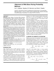
As an example, the overlap matrix constructed for propenamide is shown
(tab. 3.6). Only the SMILES C = CC(= O)N was needed for its generation
and the subsequent calculation of energy levels (fig. 3.8) and charge distribution
(fig. 3.7).
−0.03
−0.07
0.60
O
−1.02
−0.10
NH 2
Figure 3.7: Charge distribution in propenamide (in electron charges).

Table 3.6: Overlap matrix for propenamide (fig. 3.5). First and second rows are the atom and the the type of
the AO. The indices next to the atom names are given for better orientation and correspond to the indices in the
propenamide SMILES C 1 (H 2 )(H 3 ) = C 4 (H 5 )C 6 (= O 7 )N 8 (H 9 )H 10 .
C 1 H 2 C 1 H 3 C 1 C 4 C 4 H 5 C 4 C 6 C 6 O 7 C 6 N 8 N 8 H 9 N 8 H 10 O 7 O 7 C 1 C 4 C 6 O 7 N 8
sp 2 s sp 2 s sp 2 sp 2 sp 2 s sp 2 sp 2 sp 2 sp 2 sp 2 sp 2 sp 2 s sp 2 s sp 2 sp 2 p p p p p
1 .65 0 0 0 .077 0 0 0 0 0 0 0 0 0 0 0 0 0 0 0 0 0 0 0
.65 1 0 0 0 0 0 0 0 0 0 0 0 0 0 0 0 0 0 0 0 0 0 0 0
0 0 1 .65 0 .077 0 0 0 0 0 0 0 0 0 0 0 0 0 0 0 0 0 0 0
0 0 .65 1 0 0 0 0 0 0 0 0 0 0 0 0 0 0 0 0 0 0 0 0 0
0 0 0 0 1 .77.077 0 .077 0 0 0 0 0 0 0 0 0 0 0 0 0 0 0 0
.077 0 .077 0 .77 1 0 0 0 .077 0 0 0 0 0 0 0 0 0 0 0 0 0 0 0
0 0 0 0 .077 0 1 .65 0 .077 0 0 0 0 0 0 0 0 0 0 0 0 0 0 0
0 0 0 0 0 0 .65 1 0 0 0 0 0 0 0 0 0 0 0 0 0 0 0 0 0
0 0 0 0 .077 0 0 0 1 .77.077 0 .077 0 0 0 0 0 0 0 0 0 0 0 0
0 0 0 0 0 .077.077 0 .77 1 0 .068 0 .073 0 0 0 0 0 0 0 0 0 0 0
0 0 0 0 0 0 0 0 .077 0 1 .68 0 .073 0 0 0 0 .068.068 0 0 0 0 0
0 0 0 0 0 0 0 0 0 .068.68 1 .068 0 0 0 0 0 0 0 0 0 0 0 0
0 0 0 0 0 0 0 0 .077 0 0 .068 1 .73.073 0 .073 0 0 0 0 0 0 0 0
0 0 0 0 0 0 0 0 0 .073.073 0 .73 1 0 0 0 0 0 0 0 0 0 0 0
0 0 0 0 0 0 0 0 0 0 0 0 .073 0 1 .63 0 0 0 0 0 0 0 0 0
0 0 0 0 0 0 0 0 0 0 0 0 0 0 .63 1 0 0 0 0 0 0 0 0 0
0 0 0 0 0 0 0 0 0 0 0 0 .073 0 0 0 1 .63 0 0 0 0 0 0 0
0 0 0 0 0 0 0 0 0 0 0 0 0 0 0 0 .63 1 0 0 0 0 0 0 0
0 0 0 0 0 0 0 0 0 0 .068 0 0 0 0 0 0 0 1 0 0 0 0 0 0
0 0 0 0 0 0 0 0 0 0 .068 0 0 0 0 0 0 0 0 1 0 0 0 0 0
0 0 0 0 0 0 0 0 0 0 0 0 0 0 0 0 0 0 0 0 1 .38 0 0 0
0 0 0 0 0 0 0 0 0 0 0 0 0 0 0 0 0 0 0 0 .38 1 .38 0 0
0 0 0 0 0 0 0 0 0 0 0 0 0 0 0 0 0 0 0 0 0 .38 1 .26.31
0 0 0 0 0 0 0 0 0 0 0 0 0 0 0 0 0 0 0 0 0 0 .26 1 0
0 0 0 0 0 0 0 0 0 0 0 0 0 0 0 0 0 0 0 0 0 0 .31 0 1
3.4. WAVE FUNCTION ANALYSIS 29

30 CHAPTER 3. MOLECULES
E (eV)
110
✻
σ ∗ (all)
30
σ ∗ (all)
10
5
0
σ ∗ (all)
σs ∗
σ ∗ (C1 H, C 4 H, C 6 O)
a (C1 H)
σa ∗(NH)
∗(OC6 C 4 H)
σs(C ∗ 4 C 1 H) π(CCC(O)N)
σs(CNH)
∗
-10
π(CCC(O)N)
-15
⇋ ⇋⇋
π(CCC(O)N)
π(CCC(O)N)
π(CCC(O)N)
-20
⇋
⇋
⇋ ⇋ ⇋⇋ ⇋
⇋
⇋
σ a/a/s (C 1 H, C 4 H)
σ s/a (CCC)
Osp 2 σ a/s (NH)
a/s
σ(CN)
σ(CO)
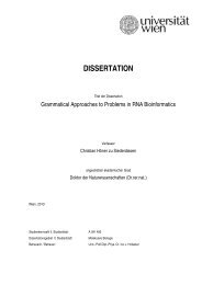
Figure 3.8: Spectrum (MO energies) of propenamide and their types. σ ∗ a (NH)
means that the MO is concentrated on the σ overlap(s) between N and the
Hs attached to it. The indices ∗ and a (antisymmetric, as opposed to s,
symmetric) indicate that the LCAO coefficients C ij (see sect. 3.1) of the
atoms N and H are of opposite sign regarding (Nsp 2 ,Hs)-pairs (∗) and of
same magnitude but opposite sign regarding (Nsp 2 ,Nsp 2 )- and (Hs,Hs)-pairs
(a). The indices on the atoms are the same as in fig. 3.6.

3.5. PERFORMANCE 31
3.5 Performance
In order to validate the energy calculation, predicted total atomization energies
(TAE) have been compared to experimental ones, see figs. 3.9 and 3.10.
Experimental TAE values are taken from [18].
Fig. 3.9 shows well how every −CH 2 − unit corresponds to an energy increment
[11]. The distance between two successive points is almost constant.
Indeed, this can be rationalized by the fact that S and H can be brought
into a quasi-block-diagonal form, every block corresponding to one −CH 2 −
unit. It follows that the total energy is proportional to the number of these
units.
Calculated TAE (kcal/mol)
1500
1000
500
1500
1000
500
500 1000 1500
500 1000 1500
Experimental TAE (in kcal/mol)
Figure 3.9: Comparison of calculated and experimental Total Atomization
Energy (TAE) for homologous series of alkanes (methane to hexane, left) and
cycloalkanes (cyclopropane to cyclohexane, right).
Fig. 3.10 shows a reasonable correlation, given the rough approximations
of the Toy Model. The same TAE are calculated for cis/trans isomers because
their are topologically equivalent (Z,Z- and E,Z- and E,E-2,4-hexadiene, for
example ). Moreover, a big part of the energy differences between the C 6 H 10
stems from electrostatic repulsion, which depends on the steric configuration
ignored by the Toy Model (see ch. 7 for improvements).
The Toy Model does obviously not include the calculation of vibrational
and rotational energy and of entropy. [18, 67] discuss methods for their
approximation. However, it seems that their contribution is small.
Highest Occupied MOs (HOMOs) of type σ instead of π are predicted for
some olefinic systems. However, this is in agreement with the results of [57,
vol. I, fig. 10.33].

32 CHAPTER 3. MOLECULES
1610
1600
Calculated TAE (kcal/mol)
1590
1580
1570
1560
1550
1520 1530 1540 1550
Experimental TAE (kcal/mol)
Figure 3.10: Plots of calculated vs. experimental TAE for C 6 H 10 isomers, in
order of increasing experimental TAE those are 1-hexyne, 2- and 3-hexyne,
3,3-dimethyl-1-butyne, 1,5-hexadiene, Z- and E-1,4-hexadiene, Z- and E-1,3-
hexadiene, Z,Z- and E,Z- and E,E-2,4-hexadiene, bicyclo[3.1.0]hexane, 4- and
3-methylcyclopentene, 1-methylcyclopentene.

3.6. FRONTIER MOLECULAR ORBITAL THEORY 33
3.6 Frontier Molecular Orbital Theory
It is natural to continue with the qualitative theory of Frontier Molecular
Orbital (FMO) theory after having used EHT for molecular property calculation.
From perturbation theory, the energy increment incurred by the
reactants A and B by interacting at the start of a reaction is the Klopman-
Salem formula [71, 99]
∆E = ∑
G ab + ∑ q(a)q(b)
ɛr ab
a∈A,b∈B a∈A,b∈B
( occ
)
∑
unocc
∑ ∑occ
unocc
∑
− F α,ζ + F α,ζ
α∈A ζ∈B α∈B ζ∈A
G ab = − ∑ ∑
(q i + q j )H ij S ij ,
i@a j@b
( ) 2
F α,ζ 2 ∑ ∑∑
∑
=
C α,i C ζ,j H ij ,
E ζ − E α
a∈A
i@a
b∈B
j@b
(3.16)
where r ab is the bond length, ɛ is the dielectric constant of the reaction
medium and α ∈ A and ζ ∈ B is an occupied and an unoccupied MO, respectively.
This increment is extrapolated in FMO theory from the initial
stage of the reaction to the transition state and may thus serve to approximate
the reaction rate. It can be derived to predict relative reactivities and
regioselectivity as described in [38]. The reactivity is then inversely proportional
to the difference of the HOMO and LUMO energies of the reactants.
The regioselectivity is determined by the MO coefficients at the reactive sites
i, such that ∑ i C HOMO,i C LUMO,i is maximal.
With the abbreviation
we obtain a four-point term
occ
F ab;a ′ b ′ = 2 ∑
W αζ
ab = ∑ i@a
α∈A
unocc
∑
ζ∈B
∑
C α,i C ζ,j H ij (3.17)
j@b
W αζ
ab W αζ
a ′ b ′
E ζ − E α
+
∑occ
α∈B
unocc
∑
ζ∈A
W αζ
ba W αζ
b ′ a ′
E ζ − E α
(3.18)
that allows us to write ∆E as an expansion of atom pairs and quadruples.
Within the approximation of the Toy Model all contributions (with the exception
of the Coulomb term) that do not belong to new bonds (or bonds

34 CHAPTER 3. MOLECULES
with increasing bond order) vanish because their overlap integrals are zero.
Thus
∆E = ∑ (
G ab + q(a)q(b) )
− F ab;ab −
∑
F ab;a
ɛr ′ b ′ (3.19)
ab
(a,b)
(a,b)̸=(a ′ ,b ′ )
where the sums run only over newly formed bonds (a, b). The same formalism
can be applied to intra-molecular reactions by setting A = B; in eq. 3.18 we
then retain only one of the two double sums (which become identical in this
case). The reactivity ∆E allows us to model regioselectivity. If more than
one subgraph isomorphism, i.e. more than one possible reaction channel, has
been found one simply has to evaluate ∆E for all of them. Then the rewrite
with the smallest ∆E value is chosen.
Eq. 3.16 has three terms which allow to classify reactions in three groups
[38, 67, ch. 2 resp. ch. 15]. The first term is mainly constant and depends
mostly on the steric configuration during a reaction. The second term is most
important for polar reactants, in charge controlled reactions. The third term
will dominate for non-polar reactants, in orbital controlled reactions. FMO
theory only considers the last term. Although its numerical contribution is
small, this approach is justified by the fact that the shapes of the HOMO and
LUMO resemble to the total electron density important for the reactivity.
Keeping in mind that MOs do not exist in reality, they are still constructs of
MO thoery useful for explaining energy differences between “real” electronic
states.
The situation can be simplified further by considering only the frontier
orbitals [46], i.e. the HOMO of one system and the LUMO of the other one.
In this case the sums in eq. 3.18 reduce to a single term. Often this is approximated
by ∆E ‡ = ξ/(E ζ −E α ) with an empirical constant ξ that depends only
on the reaction mechanism [38]. The reaction rate and activation energy are
related by Arrhenius’ law ∆E ‡ = RT ln k . The regioselectivity is determined
by the MO coefficients at the reactive sites, such that ∑ i C HOMO,i C LUMO,i
is maximal. This simplification was used for generating the two examples in
chapter 6, figs. 6.1 and 6.2.

Chapter 4
Chemical reactions
A molecule is composed of atoms that are tied together by aid
of the electrons. Atomic nuclei and electrons are not at rest but
are constantly moving. The paths of the electrons are usually
called orbitals. The forms of these orbitals are determining the
bonds between the atoms. In a reaction molecules are impinging
against each other. During the collision the electrons are influenced
by new atomic nuclei and the orbitals are changed. Some
of the bonds are broken and others are created. Afterwards, new
molecules have been formed.
The Nobel Prize in Chemistry 1981. Presentation Speech
by Professor Inga Fischer-Hjalmars of the Swedish Royal
Academy of Sciences
4.1 Graph rewriting
This section summarizes the work of Dörr [29] and [37] and explains how it
can be applied to the problem of implementing chemical reactions.
As we represented molecules as graphs, it is natural to simulate the set
of reactions by generic reactions (see sect. 2.2) in the framework of a graph
grammar [82, 97]. A graph grammar is a finite set of rules operating on
edge and vertex labeled graphs. The term “graph grammar” is rather used
for graph-generating applications. In our context, the similar term “graph
rewriting system” used for graph-transforming application is more appropriate.
Graph transformations have been studied first 30 years ago [84] for the
generation, manipulation, recognition of graphs. Four types of applications
35

36 CHAPTER 4. CHEMICAL REACTIONS
exists: the aforementioned graph grammar, unordered, ordered, and eventdriven
graph rewriting systems. The first uses a set of rules, a host graph,
and terminal (ending) labels to generate a language or for parsing. The
second consists only of a set rules and rewrites a graph without further considerations.
The third and fourth type include specifications controlling the
rewriting, for example when to stop. The Toy Model uses the event-driven
type, where the sequence of rewritings/reactions is controlled from outside,
depending on other (energy) calculations.
Graph rewriting systems have been applied to a variety of domains. Pattern
recognition and specification of database systems are easily conceivable
uses, but also less obvious approaches are possible. Visual languages might
be defined using graph transformation, and relatedly, also the semantics of
other languages or compilers. With the project PARES [97, ch. 12] there is
even an example for the application of graph grammars to art. In PARES,
the paintings of Picasso 1 are reconstructed, starting with an empty canvas,
and using derivation rules. Each rule adds new structural information, until
a typical cubist painting is obtained.
A major problem in graph rewriting is the complexity of subgraph isomorphism.
A subgraph h = (V h , E h ) of a graph g is defined by V h ∈ V g and
E h ∈ V h ×V h . An isomorphism is defined on two graphs g 1 and g 2 as the bijective
application f : V 1 → V 2 such that (u, v) ∈ E 1 ⇐⇒ (f(u), f(v)) ∈ E 2 .
The subgraph isomorphism problem is NP-complete [49] (for the graph isomorphism
problem, it is not known whether it is NP-complete). Theoretical
investigations have shown that there exists a moderately exponential bound
for the general problem [7]. More practical approaches have started with
backtracking [22], refined by reducing the search space, as reviewed by [97].
Dörr describes an algorithm in which breadth-first-search determines all
subgraphs isomorphic to the rewrite rule left-hand side. The search is implemented
as an abstract machine, i.e. a software implementation of a processor,
including an instruction set, a register set, and a model of memory.
For a faster implementation, only one abstract machine for all host graphs
is generated. Furthermore, a search strategy adapted to a subclass of graphs
rewriting systems is adopted to obtain an efficient solution, in contrast to
the general NP-complete problem. The search uses a sufficient condition for
which the algorithm performs in constant time. The condition is based on
graph properties of the graph rewriting system (sets of unique vertex labels
and strong V-structures). A rewriting system for which all rules satisfy the
condition is called Unique vertex label and Bypassing Strong V-structures
(UBS) .
1 “Computers are useless. They can only give you answers.” – Pablo Picasso

4.1. GRAPH REWRITING 37
Graphical transformations can be described in terms of graphical pre- and
post-conditions. It is possible to use a rule-based notation for this transformation.
Such a rewrite rule is a tuple r = (g l , g r , M), where the graph g l is
the left-hand side, g r is the right-hand side, and M is the set of embedding
descriptions (important for the dangling ends). The implementation used in
the Toy Model defines g l and g r by the elements of the graph no longer and
only present after the transformation, respectively, and by a context which
contains the constant element, see figs. 4.1 and 4.2.
The execution of the rewrite rule is decomposed into four steps:
• find an isomorphic subgraph (to g l )
• remove that subgraph (keeping the dangling ends in M)
• insert a new subgraph (g r )
• connect it to the rest of the graph (respecting the dangling ends from
M)
This graph rewriting formalism is very flexible and can be used to represent
chemical reactions as well as chemically impossible yet strategically
interesting reactions. It may be interesting to use scaffold replacement rules
for building a library in combinatorial chemistry, or to simulate deprotonation
implicitly, but in reality, chemical reactions do not create or destroy
atoms. A chemical reaction is the breaking, forming and changing of bonds.
Thus the number and type of atoms must remain constant, which can be
implemented by conservation of vertex labels. In analogy, the conservation of
the number of valence electrons can be imposed on rewrite rules by ensuring
conservation of total bond order. Both principles stem from the fact that
chemical reactions are stoichiometric [31, 113]:
• conservation of vertex labels : V l = V r
• conservation of total bond order : ∑ e∈E l
BO(e) = ∑ e∈E r
BO(e),
where V i and E i are the vertices and the edges of g i , and BO(e) is the bond
order of the edge e. In the example of the Diels-Alder reaction in fig. 4.2, the
first condition is met because all atoms are in the constant set, the context.
Counting the bond orders of g l (2+2+1+2) and g r (1+1+1+2+1+1) verifies
that the second condition is also satisfied, thus this rewrite rule is chemically
meaningful.
This reaction representation has the advantage of representing the reaction
itself also by graphs, and thus does not have the inherent limitations

38 CHAPTER 4. CHEMICAL REACTIONS
left graph context right graph
host graph
product graph
find left graph and context
reconnect
remove left graph
insert right graph
Figure 4.1: Graph rewriting steps.

4.1. GRAPH REWRITING 39
C
C
C
C
C
C
C
C
C
C
C
C
C
C
C
C
C
C
Left Graph
Context
Right Graph
O
O
O
O
Figure 4.2: Intramolecular Diels Alder rearrangement (iDAR). Top: rewrite
rule; since all bounds change their type during the rewrite, the context consists
of the six C-atoms only. Bottom: Application of iDAR to the synthesis
of a bridged ring system.

40 CHAPTER 4. CHEMICAL REACTIONS
of string representations, for example. It is also, of course, more flexible
and simpler than a hard-coded implementation of reactions, as complicated
reactions might be very time-consuming to encode one per one.
4.2 Graph Rewrite Engine
Dörr’s algorithm uses connected enumeration, i.e. g l must be connected. Thus
for every pair of vertices (u, v) ∈ V × V there must be a list of vertices
(v 1 . . .v n ) with v i ∈ V , such that all pairs (v i , v i+1 ) are connected by an
edge. Yet a rewrite rule corresponding to a bimolecular reactions will have
a disconnected g l , composed by two subgraphs corresponding to the two
reacting entities. The two subgraphs can not be connected by an edge, as
the two molecules are not bonded prior to reaction.
In the Toy Model, reactions are simulated by a separate Graph Rewrite
Engine (GRW). The GRW simulation of unimolecular reactions is a straight
forward application of rewrite rules to a molecule. A bimolecular reaction
or any other similar rule is split by the GRW into one half reaction rule for
each educt molecule, and a final reaction rule. The two half reaction rules
do not modify existing bonds and atoms in the molecules, they just add
“flag” nodes to the atoms that will be joined during the total reaction. They
serve to identify those reaction sites for the reactivity evaluation in sect. 3.6.
The evaluation determines which pairs of reaction sites from each of the two
reactants are joined by a temporary edge. This temporary construct is then
again submitted to the final reaction rule and transformed to the product.
Fig. 4.3 shows the reaction rules of the aldol reaction.
There are bimolecular reactions like Cannizzaro’s disproportionation [16],
olefin metathesis [127] or organic catalysis whence two products emerge. As
g r need not be connected, the final reaction rule can be adapted to this
situation.

4.2. GRAPH REWRITE ENGINE 41
O
O
O
H
Half−Rule 1
C
C
Ψ
O
H
O
O
Half−Rule 2
C
C
C
C
Ψ
Join−Rule
Ψ
Ψ
C
Ψ
Ψ
C
Left Graph
Context
Right Graph
O
+
O
O
OH
Figure 4.3: Aldol Reaction. Top: rewrite rule; the two half-rules describe
the local changes in the reacting molecules during Aldol condensation, while
the half-rule-join describes only intermolecular changes; notice the special
label Ψ, acting as anchor for the intermolecular bond to be formed. Only the
elements in black are actually contained in the rules, the other elements are
displayed to hint at their embeddings. Bottom: Application to the synthesis
of β-hydroxy-carbonyls.

42 CHAPTER 4. CHEMICAL REACTIONS

Chapter 5
Reaction networks
5.1 Network generation
The starting point for generation a CRN is an initial set of molecules L 0 .
At the present stage of development, the CRN is built exhaustively from the
network “seed” L 0 . The algorithm used can be termed “orderly generation”
for its resemblance to an algorithm of this name used for enumeration of
isomers [93, 33]. It generates the CRN by the following recursion:
Start (1) perform all unimolecular reactions on each molecule M ∈ L 0 and
put the products in a new set L ′ 1, eliminating all duplicates.
(2) perform all bimolecular reactions with each pair of molecules
(M 1 , M 2 ) ∈ L 0 × L 0 and add the products to set L ′ 1 , eliminating again
all duplicates. The last two steps are summarized by the notation
L ′ 1 = L 0 ⊗ L 0 . L i ⊗ L j means that step 1 is applied only to the first
operand L i , and step 2 on pairs (M 1 , M 2 ) ∈ L i × L j .
(3) this first iteration is completed by calculating L 1 = L ′ 1 \ L 0 .
(
Recursion (1) L ′ k+1 = ⋃k−1
)
j=0 L j ⊗ L k ∪ (L k ⊗ L k )
(2) and L k+1 = L ′ k+1 \ ⋃ L k .
Let us now consider the rewriting step for a bimolecular reaction in detail.
First the Toy Model sends the two educt graphs to the GRW. The server
then constructs all subgraph isomorphisms for the left hand side of both
half-rules for both graphs. If the list of subgraph isomorphisms for one of
the two half-rules is empty for both graphs, the rule is not applicable and
the server sends the two graphs unaltered back to the Toy Model. This case
43

44 CHAPTER 5. REACTION NETWORKS
corresponds to an “elastic collision”. Otherwise the server picks a half-rule at
random for the first graph and then a corresponding half-rule for the second
graph. This corresponds to choosing a reaction channel if there is more than
one subgraph isomorphism. Instead of picking a subgraph isomorphism at
random from the list, it is possible to consider all reaction channels and to
compute a reactivity index for each of them. The Toy Model can then pick
the reaction channel (pair of subgraph isomorphisms for the two half-rules).
The procedure for a unimolecular reaction is straightforward: the Toy Model
sends one molecule to GRW for which in analogy to the previous description
all subgraph isomorphism are constructed, and unless there is none, one
isomorphism is picked according to its reactivity.
Using the aforementioned algorithm, the CRN is likely to grow very fast.
This corresponds for example to the very complex network of elementary
reactions constituting a polymerization. The repetitive Diels-Alder networks
in fig. 6.1 suffers from this problem. However, there are techniques to simplify
such a network called model reduction techniques [43]. Reactions may
be removed from the CRN during or after generation, or formally “lumped”
together before, on the basis of e.g. energetic criteria. It is particularly efficient
to perform CRN generation and reduction simultaneously [33, 43],
as uninteresting reactions generate products that may further undergo uninteresting
reactions and so on. Detailed model reduction eliminates such
reactions before they can develop further. In the Toy Model, detailed reduction
is performed by selecting reactions according to their enthalpy, their
activation energy, or both.
5.2 Representation
A chemical reaction network (CRN) is a set of molecules linked together by
reactions leading from one subset to another.
A chemical reaction
aA + bB + · · · → vV + wW + · · · (5.1)
can be described as a directed hypergraph [131]. A hypergraph H(V, E)
is a set of vertices and a set of hyperedges, where vertices are elements v i
and hyperedges are pairs of lists of vertices ({u i }, {v i }) with u i ∈ ∏ V and
v i ∈ ∏ V defining connected vertices. The term directed specifies that the
order of vertices in the definition of an edge or a hyperedge is important. The
chemical species are the vertices. A reaction forms a hyperedge ρ ∈ E that
connects educts with products. A CRN is then represented by a hypergraph
with hyperedges for each reaction.

5.3. NETWORK PROPERTIES 45
O 3
NO 3
NO 2
O 2
O 3
NO 3
NO 2
O 2
Figure 5.1: Representation of a chemical reaction NO 2 + O 3 → NO 3 + O 2 as
a directed hypergraph H(V, E). The chemical species are the vertices X ∈ V .
Each reaction is represented by a single directed hyperedge connecting educts
with products. Directed hypergraphs are conveniently displayed as bipartite
directed graphs. Here the reactions are represented as a second type of
vertices. Directed edges connect educts with the reaction vertex and the
reaction vertex with products of the reaction.
Alternatively, a CRN can be described as a bipartite directed graph [9,
132, sect. 2.3.2]. A bipartite graph V(V, E) can be partitioned into two sets
of vertices V 1 and V 2 satisfying V = V 1 ∪ V 2 and V 1 ∩ V 2 = ∅, such that there
is no edge e = (u, v) with u ∈ V 1 and v ∈ V 2 . In the bipartite directed graph,
molecules are represented by a class of species vertices, V 1 , and the reactions
form a second class V 2 of vertices, reaction vertices. Directed edges then
connect the educt vertices with the reaction vertex and the reaction vertex
with the product vertices, as in fig. 5.1.
5.3 Network properties
It is finally possible to extract properties of the generated CRNs. Ref. [1] reviews
interesting graph-theoretic properties of networks. Most of the research
is concentrated on the degree distribution, the small-world phenomenon, and
the cliquishness in networks. In sect. 6.3, small-world and scale-free networks
are described. Both network types may be combined with special cycle distributions,
for example an abundance of short cycles [55].
The following characteristics are needed (n and m are the number of
nodes and edges) :
• 〈k〉 = 2 m , the average node degree,
n
• 〈L〉, the average length of the shortest path between to nodes, and
edges between i-neighbors
• 〈C〉, where C i = 2 is the clustering coefficient. It
i-neighbors(i-neighbors−1)
describes how much the neighborhood of a node resembles to a complete
graph, the cliquishness.

46 CHAPTER 5. REACTION NETWORKS
Bipartite graph −→ Substrate graph
O 3
NO 3
NO 2
O 2
−→
O 3
NO 3
NO 2
O 2
−→
Figure 5.2: One-mode projection from a bipartite graph to a substrate graph.
However, 〈C〉 is obviously not defined in a bipartite graph. Thus a different
representation from the one in figs. 5.1, 6.1 and 6.2 has to be used. The
substrate graph [36] is appropriate and obtained from the bipartite graph
representation by a one-mode projection (fig. 5.2, [117]). In the substrate
graph, all molecules occurring together in a reaction are connected by an
edge. It has to be noted that information is lost by projection. The substrate
graph is undirected, because elements downstream a reaction pathway
may affect elements upstream. For example, even in irreversible reactions,
product concentration can affect the reaction rate.
An algebraic representation of a CRN is the stoichiometric matrix [132].
In a stoichiometric matrix N, columns correspond to reactions and rows to
species. The entry N ij is the stoichiometric coefficient, i.e. the number of
molecules of i participating in the reaction j. The coefficient is positive
or negative depending on whether the species is produced or consumed in
the reaction. Reversible reactions are considered as two separate symmetric
reactions in opposing directions. Although reactions containing the same
species on both sides can be represented by a hyperedge in hypergraph or a
cycle of length 2 in a bipartite graph, there is no appropriate stoichiometric
coefficient. Nevertheless, reactions of this type, like autocatalytic reactions,
can be decomposed into tractable elementary steps, which often corresponds
to reality. The stoichiometric matrix is the starting point for control analysis
and flux analysis. The program METATOOL [102] derives elementary modes

5.3. NETWORK PROPERTIES 47
(see ch. 1) from networks representing metabolic pathways, in which the
reactions are controlled by implicit enzymes.

48 CHAPTER 5. REACTION NETWORKS

Chapter 6
Computational results
When the three components molecules, reactions, and network simulation
are put together, it is possible to build a CRN performing molecular property
prediction and model reduction on the fly, given only a list of initial
SMILES. For the following CRNs, regioselectivity was simulated using the
simple equations described at the end of section 3.6.
6.1 Repetitive Diels-Alder reactions
The Diels-Alder reaction [25] has been extensively studied thanks to its importance
in natural products synthesis and because it is easily tractable by
simple semi-empirical methods. It is the typical test reaction for a semiempirical
quantum calculation methods such as ours, and furthermore for
the numerous approaches of reaction description [110]. It involves the reaction
between two linear π-systems of length 2 and 4, called dienophiles
and dienes, and is thus called a [2+4]-cycloaddition. The product is again a
dienophile and may react again in a Diels-Alder reaction, then termed repetitive.
Indeed, the reaction is used for the synthesis of polymers [80]. The
CRN in fig. 6.1 is obtained by repetitive Diels-Alder reactions of a simple
initial mixture of dienes and dienophiles.
The rewrite rule is a bimolecular variant of the one described in fig. 4.2
(see appendix B). The simple constraints derived from FMO lead to a reaction
respecting the Woodward-Hoffmann rules [126]. Depending on which
choice makes |∆E FMO | smaller, the HOMO of the diene or dienophile reacts
with the LUMO of the complementary species. The orientation of the reactants
to each other is determined by the FMO coefficients. Model reduction
consisted in producing only one of regioisomers instead of both. A further
reduction was introduced by an enthalpy threshold of 20 eV.
49

O
O
O
O
O
O
O
O
O
O
O
O
O
O
O
O
O
O
O
O
O
O
O
O
O
O
O
O
O
O
50 CHAPTER 6. COMPUTATIONAL RESULTS
O
2.66
O
O
O
O
1.44
O
O
O
O
O
2.66
2.66
O
O
O
2.66
O
O
O
O
O
2.13
1.44
O
O
O
2.66
5.71
O
O
O
O
1.44
1.44
O
1.44
O
4.47
2.66
1.44
O
O
O
1.44
O
2.66
O
4.46
4.47
O
O
4.47
4.46
4.47
O
O
O
O
2.66
O
4.46
O
O
O
O
O
O
O
1.44
O
O
O
O
1.17
1.17
1.17
O
O
4.46
1.17
1.17
O
O
O
1.33
O
O
O
O
O
3.37
3.72
O
1.45
Figure 6.1: Network of Diels-Alder reaction constructed with 3 iterations of
the orderly generation algorithm. The initial mixture consists of cyclobutadiene,
ethenol, phtalic anhydride, methylbutadiene, and cyclohexa-1,3-diene.
Each rectangle represents one reaction, its label indicates the reaction rate
using the proportionality constant ξ from [101]. The correlation used is
∆E ‡ = 200/∆E FMO − 30.
6.2 The formose reaction
The synthesis of sugars from formaldehyde under alkaline conditions (“formose
reaction”) was discovered more than a century ago [15]. It is one of
the earliest examples of a reaction network that is collectively autocatalytic
in the sense that the reaction products catalyze their own formation. The
condensation of formaldehyde proceeds by means of repeated aldol condensations
and subsequent dismutations [13, 85]. The formose reaction has been
studied in much detail because of its importance as a potential prebiotic
pathway [47]. Formaldehyde has been found in the reaction mixture of abiogenesis
experiments, right from the start in Miller-Urey’s Electric Discharge

O
O
O
O
O
O
O
O
O
O
O
O
O
O
O
O
O
O
O
O
O
O
O
O
O
O
O
O
O
O
O
O
O
O
O
O
O
O
O
O
O
O
O
O
O
O
O
O
O
O
O
O
O
O
O
O
O
O
O
O
O
O
O
O
O
O
O
O
O
O
O
O
O
O
O
O
O
O
O
O
O
O
O
O
O
O
O
O
O
O
O
O
O
O
O
O
O
O
O
O
O
O
O
O
O
O
O
O
O
O
O
O
O
O
O
O
O
O
O
O
O
O
O
O
O
O
O
O
O
O
O
O
O
O
O
O
O
O
O
O
O
O
O
O
O
O
O
O
O
O
O
O
O
O
O
O
O
O
O
O
O
O
O
O
O
O
O
O
O
O
O
O
O
O
O
O
O
O
O
O
O
O
O
O
O
O
O
O
O
O
O
O
O
O
O
O
O
O
O
O
O
O
O
O
O
O
O
O
O
O
O
O
O
O
O
O
O
O
O
O
O
O
6.2. THE FORMOSE REACTION 51
2.51
O
O
4.18
O
0.36
0.36
O
O
O
O
O
O
O
O
0.26
O
O
O
0.04
0.26
O
O
O
O
O
0.36
O
O
O
O
0.03
O
O
O
0.26
0.26
O
O
O
O
2.51
O
4.17
O
O
O
O
0.03
0.26
O
O
O
O
O
O
O
O
2.51
O
O
O
O
Figure 6.2: Formaldehyde condensation reaction network. The initial mixture
consists of formaldehyde H 2 CO and glycol aldehyde CH 2 OH − CHO and
reacts via aldol condensations and dismutations. The aldol condensation
was simulated by the condensation of a keto with an enole group. In order
to account for cyclization, which limits the network, we do not permit
carbon chains with more than four members to undergo further aldol condensations.
The network generation algorithm thus converges already after
two iterations. Reaction rates are computed using the proportionality
constant ξ for nucleophilic substitution from [71]. The correlation used is
∆E ‡ = 28/∆E FMO − 10.
Experiment [115]. It is thus conceivable that the formose reaction is the
origin of biological sugars.
The network produced by the Toy Model is shown in Fig. 6.2. It is built

52 CHAPTER 6. COMPUTATIONAL RESULTS
from a mixture of formaldehyde and glycol. The first condensation step
yielding glycol from formaldehyde is assumed implicitly. The rewrite rule
used is a variant of the one described in fig. 4.3. In order to account for
cyclization, and so to reduce the network, carbon chains with more than four
members, or two chains with four members were not permitted to further
undergo aldol condensation. Furthermore, although more than 40 different
sugars have been identified in the experimental reaction mixture [24], condensation
was restricted to enoles with a primary acid hydrogen. Due to
this model reduction, the algorithm converged after only two iterations. The
Toy Model could be made more accurate by a Monte Carlo CRN generation.
It would have the same limits implicitly because unimolecular cyclization is
by far faster than bimolecular aldol condensation. This is equivalent to the
systematic model reduction described by [43].
6.3 Graph-theoretic properties
For assessing 〈L〉 and 〈C〉, we need to compare them to the results for random
Erdös-Renyi graphs:
〈L rand 〉 ≈ ln n
ln 〈k〉
〈k〉
〈C rand 〉 =
(n − 1)
Tab. 6.1 compares the network characteristics of the Diels-Alder, the
Formose, and the E. coli metabolic network. They are all sparse graphs, i.e.
they have much fewer edges than complete graphs, reflected by m ≪ n(n−1)
2
or 〈k〉 ≪ n. Sparse networks are very common, ranging from the network
of acquaintances to a neural network. In both cases, there are only few
connections at each node.
The small-world phenomenon [118, 119] is also widespread, and applies
for instance to the network of acquaintances. In the latter example, it describes
the fact that every person is acquainted to another over “six degrees
of separation”, in average. More generally, it means that the average shortest
path between two nodes in a network is small. An important application is
the propagation of diseases, where the small-world property leads to a rapid
spread. From the networks of tab. 6.1, only Diels-Alder and E. coli fulfill the
conditions 〈C〉 ≫ 〈C rand 〉 and 〈L〉 ≤ 〈L rand 〉 and thus are strictly small-world
networks. The Formose reaction network includes many non-reactive species
with respect to keto-enol condensation, which leads to small cliquishness and
longer paths.

6.3. GRAPH-THEORETIC PROPERTIES 53
Table 6.1: Characteristics of the two example CRNs and the substrate graph
of the E. coli energy and biosynthesis metabolism [36].
nodes 〈k〉 〈L〉 〈L rand 〉 〈C〉 〈C rand 〉
Formose 48 3.25 3.55 3.28 0.15 0.068
Diels-Alder 40 4.65 2.15 2.40 0.72 0.11
E. coli 282 7.35 2.9 3.04 0.32 0.026
Finally, the degree distributions have been calculated (fig. 6.3). Both
networks are scale-free, i.e. their degree distributions follow a power law.
The cumulative representation of fig. 6.3 is equivalent to ∫ ∞
P(x)dx vs. k.
k
The regression ∫ ∞
P(x)dx ∼ k
k−1.19 is consistent with the values reported in
[10]. The explanation of the origin of scale-freeness therein can be applied
to the present examples. It relies on two generic mechanisms. First, the
networks grows from on an initial set of nodes by continuous addition of new
nodes. Indeed, in the present case, there is an initial list of molecules, and the
networks is built by adding molecules at every iteration (sect. 5.1). Second,
the networks grows by preferential attachment, i.e. new nodes are preferably
attached to nodes with high degree, or in the case of molecules, species
who have already spawned many new other species are especially reactive
and more likely to produce new molecules at each iteration. The power-law
regression for the Formose reaction network fails for high k. The theoretical
Poisson distribution for random graphs with high n, P(k) = e −〈k〉 〈k〉 k
, also
k!
fails in this range. A degree distribution following a truncated power law has
been referred to as broad-scale [3].

54 CHAPTER 6. COMPUTATIONAL RESULTS
100
Cumulative degree distribution
10
1
1 10 100
Degree
100
Cumulative degree distribution
10
1
1 10
Degree
Figure 6.3: Cumulative degree distribution of repetitive Diels-Alder (top) and
the Formose reaction network (bottom). Datapoints are ranked by decreasing
degree. Datapoints, power-law regressions, and theoretical Poisson distribution
are represented by □, solid, and dashed lines. Regressions: y = 68x −1.19
with r 2 = 0.92 (top), y = 57x −1.19 with r 2 = 0.87 (bottom).

Chapter 7
Conclusion and Outlook
The present Toy Model is at least close to a minimal implementation of
an artificial chemistry exhibiting what we consider the defining features of
“real” chemistry. Molecules were represented only by their connectivity information
and atom types, as labeled graphs, and their energy was defined
along the lines of quantum chemistry, using an extremely simplified function.
This energy model forms the basis of full-fledged chemical thermodynamics
and kinetics. Chemical reactions are implemented as graph rewriting rules
that have to obey the principle of conservation of matter. These features
distinguish the Toy Model from artificial chemistries that are defined on abstract
algebraic structures such as the λ calculus, Turing machines, or term
rewriting. The application of the model to examples of complex organic and
prebiotic chemistry allowed an quasi-ab initio simulation of the resulting
networks and prediction of their properties. Now the emergence of generic
properties of CRNs can be studied given only starting material, generic reactions
and atom and bond parameters. A true ab initio simulation would not
need the introduction the latter parameters for the energy calculation and
would simulate reactions without even specifying generic reactions. Yet both
“educated guesses” are founded on the results of quantum chemistry and
synthetic chemistry, and their validity could be estimated by the judicious
comparison of predicted to experimental results.
A number of extensions of the present Toy Model are desirable. For
instance, the addition of the corresponding parameters (see appendix A)
would extend the current implementation of the model, considering only
molecules composed of C, H, O, and N, to an expanded set of chemical
elements, most importantly S, P, Si, and the halogens. The inclusion of
charged particles and radicals also does not seem to pose problems in the
current framework. Charges situated on specific atoms can be indicated in
SMILES, e.g. HC([O−]) = O. In fact, it does not matter to which atom the
55

56 CHAPTER 7. CONCLUSION AND OUTLOOK
charge is attributed at the beginning, the correct charge distribution is a byproduct
of the energy calculation (see sect. 3.4). Additional types of chemical
bonds, in particular hydrogen bonds and the “three center bonds” common
in boron compounds can be approximated by the orbital graph formalism
(for boranes, a common object of MO study, see [54, 63, 70]).
The interaction of a molecule with a more complex environment, in particular
a solvent, is easily incorporated into the Toy Model using an implicit
solvation model [23] such as Kirkwood’s equation
∆G solv = − ɛ − 1 µ 2
2ɛ + 1 a . (7.1)
3
Here a is the radius of the molecule and µ is its dipole moment and ɛ is
the dielectric constant of the medium. Both a and µ have to be replaced
by appropriate graph descriptors. For example a could be replaced by the
Wiener index [56, 123], with a proper normalization. A topological index for
vertex weighted graphs could serve as a “graph theoretical dipole moment”.
The reactivities from eq. 3.16 can be translated into reaction rate constants,
e.g. using Arrhenius’ law. An alternative approach to determining
rate constants is QSPR [33]. This class of models is, however, of limited
interest for our purposes because it is restricted to reaction mechanism for
which a sufficient amount of experimental data is available. This method
would involve the calculation of descriptors. For steric descriptors, like the
aforementioned dipole moment, e.g. graph-theoretic approximations have to
be used. In connection to this, an interesting application of the Toy Model
would be QSMR for the prediction of CRNs built during the metabolization
of a xenobiotic [32]. However, this would require that g l in the rewrite rule
also incorporates descriptors.
The reaction scheme from sect. 4.2 could be modified to select a reaction
channel with a probability proportional to its Boltzmann weight e −∆E/RT , i.e.
according to Arrhenius’ law. This would be the natural starting point for the
stochastic simulation of a reaction network, e.g. using Gillespie’s approach
[52, 51, 48]. There, the exact time evolution of a spatially homogeneous
mixture of molecular species, interacting through a specified set of coupled
chemical reaction channels, is integrated numerically.
It is also possible to plug the Toy Model into existing reactors like Continuous-Stirred-Tank
Reactors (CSTR) [92, 122], or Monte Carlo simulations
[6]. As stochastic methods are particularly useful for stiff systems and systems
with very small quantities, they are traditionally applied to biological
systems. Chemical applications rather make use of the numerical integration
of ordinary differential equations (ODE) to simulate the evolution of a CRN.

Using the rules of mass action kinetics [34, 64], the ODEs describing a network
can be derived from the CRN while it is produced by the Toy Model
[28]. The analysis of an ODE simulation can be further refined by methods
such as chemical and statistical lumping, sensitivity analysis and systematic
model reduction [43].
The Toy Model implements chemical reactions as explicit rewrite rules. In
principle it is possible to simulate the collision of two molecules by assigning
a collection of potential new bonds between them. Since the corresponding
reactivity ∆E and the over-all reaction energy can be computed, one could
in principle simulate reactions at this level. The computational cost would
be immense, however. Nevertheless, one could use collision simulations to
search for new reaction mechanism. This might be of particular interest when
the Toy Model is used to explore “exotic chemistries” or chemical dynamics.
The energy calculation in the Toy Model includes a few empiric parameters
(see appendix A). The parameters have been adjusted so as to reproduce
the correct ordering of the chemical classes alkanes, alkenes and alkynes
within an energy ranking of isomers. The parameters are bound to influence
the enthalpy of reactions and may thus also affect the properties of the resulting
CRN. The simulation of prebiotic chemistry can be executed with those
parameters varying. The dependency of properties on these parameters could
provide a measure for the stability and robustness of the network.
Other improvements and extensions of the three components (molecules,
reactions, networks) of the Toy Model include for molecules:
(i) use the methods in [19] to accelerate the energy calculation, improve
its accuracy by the methods of [4, 5, 94, 96],
(ii) implement cis/trans isomery using the SMILES “/\” notation,
for reactions:
(i) use the BEP/Hammond/Marcus equation for ∆E ‡ calculation, or derive
it from the energy of intermediary transition structures,
(ii) parallelize the Toy Model by setting up one server per reaction ,
(iii) simulate catalysis by proteins, e.g. peptidase by catalytic triade, or by
topological pharmacophore descriptors [74],
(iv) implement retrosynthetic steps [86, ch. 14.2] and common organic reactions
(see appendix C) as rewrite rules,
for networks:
(i) use the planarity test [98] to limit networks (may not be sufficient),
(ii) submit simulated CRNs to classification [110],
(iii) simulate CRNs of organic catalysts [76] (e.g. polyenes), of other pre- or
exobiotic chemistries [30] (e.g. tholin chemistry), of typical chemical engineering
examples (e.g. polystyrene [125]), and of starburst molecules,
57

58 CHAPTER 7. CONCLUSION AND OUTLOOK
dendrimers and other polymers [80].
In summary, the Toy Model is now able to generate artificial chemistries and
chemical reaction networks with few given parameters. The implementation
is straightforward and intuitive, especially for the reaction simulation and
the energy calculation. The latter is simple but more sophisticated than
a biased knowledge-based calculation. The resulting networks can be used
for exploring generic properties and their study may be extended to related
areas.

Appendix A
Parameters
The energy calculation in the Toy Model is parametrized in terms of ionization
energies I j and overlap integrals S ij of the usual Slater-type hybrid
orbitals. The parameters S ij needed for the energy calculation (see ch. 3)
have been obtained from the tables in [81], using the formulae for the overlap
of hybridized orbitals therein.
The bond lengths in tab. A.1, needed for this calculation were obtained
from the atom radii in [57, vol. III, sect. 3.1.1] and further refined by comparison
with [2].
Tab. A.2 lists the values of S ij that apply to σ overlaps of hybridized
orbitals that are oriented toward each other along a bond (upper left scheme
in Fig. 3.4) and to π overlaps between p orbitals. The overlap integrals S ij
depend only on the type and orientation of the involved orbitals.
In the current implementation, the overlap parameters are arranged in a
matrix S whose elements are lists of length 3. The rows and columns of the
Table A.1: Bond lengths depending on hybridization of bonding atoms. +
indicates guessed values.
H C N O
s sp 3 sp 2 sp sp 3 sp 2 sp sp 3 sp 2
H s 0.74 1.01 1.07 1.056 1.01 1.02 +1.01 0.96 0.97
C sp 3 1.54 1.52 1.46 1.47 +1.45 +1.43 1.43 +1.37
C sp 2 1.34 1.32 +1.33 1.29 +1.26 +1.29 1.23
C sp 1.21 +1.22 +1.19 1.15 +1.18 +1.12
N sp 3 1.40 +1.32 1.25 1.30 +1.26
N sp 2 1.24 +1.17 +1.22 1.18
N sp 1.10 +1.15 +1.11
59

60 APPENDIX A. PARAMETERS
matrix obviously correspond to the type of the AO. The position in the list
corresponds to the type of the overlap, where S[0] is a σ-overlap, S[1] is a
π-, a hyperconjugation-, or an indirect overlap, and S[2] is a semi-direct or
a fictitious overlap (see sect. 3.2).
Table A.2: Parameters for the graph orbital model. The top line gives the
Coulomb integrals I for the atom orbitals that are currently implemented.
Overlap integrals are listed separately for σ and π bonds. Semi-direct and
indirect overlaps and banana-bonds in constrained rings are parametrized as
the product of the bonding interaction with a scaling factor (see tab. 3.2).
σ H C N O
s sp 3 sp 2 sp sp 3 sp 2 sp sp 3 sp 2
I -13.6 -13.9 -14.5 -15.4 -16.6 -17.6 -19.7 -19.2 -20.6
H s 0.75 0.69 0.65 0.66 0.62 0.63 0.63 0.55 0.57
C sp 3 0.69 0.65 0.67 0.71 0.60 0.63 0.65 0.54 0.57
C sp 2 0.65 0.67 0.77 0.80 0.70 0.73 0.77 0.64 0.68
C sp 0.66 0.71 0.80 0.87 0.77 0.80 0.84 − −
N sp 3 0.62 0.60 0.70 0.77 0.58 0.61 0.65 0.63 0.67
N sp 2 0.63 0.63 0.73 0.80 0.61 0.70 0.73 0.63 0.67
N sp 0.63 0.65 0.77 0.84 0.65 0.73 0.82 − −
O sp 3 0.55 0.54 0.64 − 0.63 0.63 − − −
O sp 2 0.57 0.57 0.68 − 0.67 0.67 − − −
π C N O
p p p
I -11.4 -13.4 -14.8
C 0.38 0.31 0.26
N 0.31 0.31 0.26
O 0.26 0.26 0.26

Appendix B
GRW
GRW is implemented in Haskell, a lazy functional programming language
[111]. Since it is not easy to glue together pieces of code written in functional
and imperative programming languages (e.g. C), the engine is designed as
client/server application. The client sends a graph to the server, which performs
the rewrite step and sends the transformed graph back to the client.
The rewrite behavior of the server only depends on the set of rewriting rules
which are read from a file at server startup. This program architecture allows
us to easily fit the rewrite engine to the needs of a particular task by simply
changing the client. The server can be run in two rewriting modes: random
rewrite and priority rewrite. In the former mode a rewrite rule is picked at
random from the set of potentially applicable rules, while in the latter mode
the rule with the highest “priority value” is chosen.
The graph rewrite rules are conveniently specified using the Graph Meta
Language (GML) [90]. The specification of the Diels Alder reaction is, for
example:
# Diels Alder
rule [
context [
node [ id 1 label "C" ]
node [ id 2 label "C" ]
node [ id 3 label "C" ]
node [ id 4 label "C" ]
node [ id 5 label "C" ]
node [ id 6 label "C" ]
]
left [
edge [ source 1 target 2 label "=" ]
61

62 APPENDIX B. GRW
edge [ source 2 target 3 label "-" ]
edge [ source 3 target 4 label "=" ]
edge [ source 5 target 6 label "=" ]
]
right [
edge [ source 1 target 2 label "-" ]
edge [ source 2 target 3 label "=" ]
edge [ source 3 target 4 label "-" ]
edge [ source 4 target 5 label "-" ]
edge [ source 5 target 6 label "-" ]
edge [ source 6 target 1 label "-" ]
]
]

Appendix C
Organic reactions
Fromhttp://www.liv.ac.uk/Chemistry/Links/reactions.html and [86]:
- Ester Condensation
- Acryloin Condensation
- Aldol Condensation
- Baeyer-Villiger Rearrangement
- Beckmann Rearrangement
- Benzoin Condensation
- Birch Reduction
- Cannizzaro Reaction
- Chichibabin Reaction
- Claisen Condensation
- Claisen Rearrangement
- Cope Rearrangement
- Diels Alder Reaction
- Dienone Phenol Rearrangement
- Friedel Crafts Reaction
- Gabriel Synthesis
- Hell-Vollard-Zelimsky Halogenation
- Hofmann Rearrangement
63

64 APPENDIX C. ORGANIC REACTIONS
- Kiliani-Fischer Synthesis
- Knoevenagel Condensation
- Koenigs-Knorr Synthesis
- Mannich Reaction
- Meerwein-Ponndorf-Verley Reduction
- Michael Condensation
- Reformatskii Reaction
- Wagner-Meerwein Rearrangement
- Wittig Reaction
- Wolff-Kishner Reduction
- Wurtz Reaction
or
- Basic/Nucleophilic
- Acidic/Electrophilic
- Electrophilic Aromatic Substitution (EAS),
- Radical
- Heterocyclic
- Pericyclic
- Oxidative/Reductive
- Carbene
- Organometallic
- Photochemical

Bibliography
[1] R. Albert and A.-L. Barabasi. Statistical mechanics of complex networks.
Rev. Mod. Phys., 74:47–97, 2002.
[2] N. W. Alcock. Bonding and Structure. Ellis Horwood, 1990.
http://www.iumsc.indiana.edu/radii.html.
[3] L. A. N. Amaral, A. Scala, M. Barthelemy, and H. E. Stanley. Classes
of small-world networks. Proc. Nat. Acad. Sci., 97:11149–11152, 2000.
[4] A. B. Anderson. Electron density distribution functions and the ASED-
MO theory. Int. J. Quant. Chem., 49:581–589, 1994.
[5] A. B. Anderson and R. Hoffmann. Description of diatomic molecules
using one lectron configuration energies with two-body interactions. J.
Chem. Phys., 60:4271–4273, 1974.
[6] A. P. Arkin. Synthetic cell biology. Curr. Opin. Biotech., 12:638–644,
2001.
[7] L. Babai. Lecture Notes in Computer Sciences : Fundamentals of Computation
Theory, chapter Moderately exponential bound for graph isomorphism,
pages 34–50. Springer, 1981.
[8] R. J. Bagley and J. D. Farmer. Spontaneous emergence of a
metabolism. In C. G. Langton, C. Taylor, J. D. Farmer, and S. Rasmussen,
editors, Artificial Life II, pages 93–140, Redwood City, CA,
1992. Addison-Wesley.
[9] A. A. Balandin. Multiplet theory of catalysis: Theory of hydrogenation.
Classification of organic catalytic reactions. Algebra applied to strucutral
chemistry, volume 3. Moscow State Univ., 1970. in Russian.
[10] A.-L. Barabasi and R. Albert. Emergence of scaling in random networks.
Science, 286:509–512, 1999.
65

66 BIBLIOGRAPHY
[11] S. Benson. Thermochemical kinetics: methods for the estimation of
thermochemical data and rate parameters. Wiley, New York, 1968.
[12] W. Braun, R. Fugmann, and W. Vaupel. Zur Dokumentation chemischer
Forschungsgebiete. Angew. Chem., 73:745–751, 1961.
[13] R. Breslow. On the mechanism of the Formose reaction. Tetrahedron
Lett., 21:22–26, 1959.
[14] A. C. Brown. On the theory of chemical combination. Master’s thesis,
University of Edinburgh, UK, 1864.
[15] A. Butlerow. Formation synthétique d’une substance sucrée. C. R.
Acad. Sci., 53:145–147, 1861.
[16] S. Cannizzaro. Über den der Benzoësäure entsprechenden Alkohol.
Liebigs Ann. Chem., 88:129–130, 1853.
[17] A. Cayley. On the mathematical theory of isomers. Philos. Mag.,
47:444–446, 1874.
[18] Computational chemistry comparison and benchmark database, release
6a, May 2002. http://srdata.nist.gov/cccbdb/.
[19] M. Challacombe. A simplified density matrix minimization for linear
scaling self-consistent theory. J. Chem. Phys., 110:2332–2342, 1999.
[20] A. Church. A set of pustulates for the foundation of logic. Annals of
Math. (2), 33:346–366, 1932.
[21] B. L. Clarke. Stoichiometric network analysis. Cell Biophys., 12:237–
253, 1988.
[22] D. C. Corneil and C. C. Gotlieb. An efficient algorithm for graph
isomorphism. J. ACM, 17:51–64, 1970.
[23] C. J. Cramer and D. G. Truhlar. Implicit solvation models: Equilibria,
structure, spectra, and dynamics. Chem. Rev., 99:2161–2200, 1999.
[24] P. Decker, H. Schweer, and R. Pohlmann. Bioids. X. Identification
of formose sugars, presumably prebiotic metabolites, using capillary
gas chromatography/gas chromatography-mass spectroscopy of
n-butoxime trifluoroacetates on OV-225J. J. Chromatogr., 225:281–
291, 1982.

BIBLIOGRAPHY 67
[25] O. Diels and K. Alder. Synthesen in der hydroaromatischen Reihe.
Liebigs Ann. Chem., 460:98–122, 1928.
[26] P. Dittrich, J. Ziegler, and W. Banzhaf. Artificial chemistries - a review.
Artificial Life, 7:225–275, 2001.
[27] P. Dittrich and W. Banzhaf. Self-evolution in a constructive binary
string system. Artificial Life, 4:203–220, 1998.
[28] D. J. Dooling. Converting reaction mechanisms into ordinary differential
equations suitable for integration.
http://winnie.chem-eng.nwu.edu/software/ode.html.
[29] H. Dörr. Efficient Graph Rewriting and Its Implementation. Springer-
Verlag, Berlin Heidelberg, 1995.
[30] K. Dose and H. Rauchfuss. Chemische Evolution und der Ursprung
lebender Systeme. Wiss. Verlagges. Stuttgart, 1975.
[31] J. Dugundji and I. Ugi. An algebraic model of constitutional chemistry
as a basis for chemical computer programs. Top. Curr. Chem., 39:19–
49, 1973.
[32] S. Ekins, M. J. de Groot, and J. P. Jones. Pharmacophore and threedimensional
quantitative structure activity relationship methods for
modeling cytochrome P450 active sites. Drug Metab. Disp., 29:936–
944, 2001.
[33] J.-L. Faulon and A. G. Sault. Stochastic generator of chemical structure.
3. Reaction network generation. J. Chem. Inf. Comput. Sci.,
41:894–908, 2001.
[34] M. Feinberg. Chemical Reactor Theory - A Review, chapter Mathematical
Aspects of Mass Action Kinetics. Prentice-Hall, Inglewood Cliffs,
NJ, 1977.
[35] D. Fell. Understanding the Control of Metabolism. Number 2 in Frontiers
in Metabolism. Portland Press, London, 1997.
[36] D. Fell and A. Wagner. The small world inside metabolic networks.
Proc. R. Soc. Lond. Ser. B, 268:1803–1810, 2001.
[37] C. Flamm. Graph rewrite ?!@$+*.
http://www.tbi.univie.ac.at/Bled/Slides/xtof.pdf, 2002.

68 BIBLIOGRAPHY
[38] I. Fleming. Frontier Orbitals and Organic Chemical Reactions. Wiley:
New York, 1976.
[39] E. Fontain and K. Reitsam. The generation of reaction networks with
rain. Part 1. The reaction generator. J. Chem. Inf. Comput. Sci.,
31:96–100, 1991.
[40] W. Fontana. Algorithmic chemistry. In C. G. Langton, C. Taylor, J. D.
Farmer, and S. Rasmussen, editors, Proc. Workshop on Artificial Life
(ALIFE ’90), volume 5 of Santa Fe Institute Studies in the Sciences
of Complexity, pages 159–210, Redwood City, CA, USA, Feb. 1992.
Addison-Wesley.
[41] W. Fontana and L. W. Buss ’The arrival of the fittest’: Toward a
theory of biological organization. Bull. Math. Biol., 56:1–64, 1994.
[42] W. Fontana and L. W. Buss The barrier of objects: From dynamical
systems to bounded organization. In J. Casti and A. Karlqvist,
editors, Boundaries and Barriers, pages 56–116, Redwood City, MA,
1996. Addison-Wesley.
[43] M. Frenklach. Modeling of large reaction systems. In J. Warnatz and
W. Jäger, editors, Complex chemical reaction systems, mathematical
modelling and simulation, volume 47 of Springer Series in Chemical
Physics, pages 2–16. Springer-Verlag, Berlin, 1987.
[44] R. Fugmann. In Proceedings of the IUPAC Congress 1959, pages 331–
341, 1959.
[45] S. Fujita. Description of organic reactions based on imaginary transition
structures. 1. Introduction of new concepts. J. Chem. Inf. Comput.
Sci., 26:205–212, 1986.
[46] K. Fukui, T. Yonezawa, and H. Shingu. A molecular orbital theory
of reactivity in aromatic hydrocarbons. J. Chem. Phys., 20:722–725,
1952.
[47] N. W. Gabel and C. Ponnamperuma. Model for origin of monosaccharides.
Nature, 216:452–455, 1967.
[48] C. W. Gardiner. Handbook of Stochastic Methods. Springer, Berlin,
1985.
[49] M. R. Garey and D. S. Johnson. Computers and Intractability. W. H.
Freeman and Co., New York, 1979.

BIBLIOGRAPHY 69
[50] J. Gasteiger and A. Herwig. Simulation of organic reactions: From
the degradation of chemicals to combinatorial synthesis. J. Chem. Inf.
Comput. Sci., 40:482–494, 2000.
[51] M. A. Gibson and J. Bruck. Efficient exact stochastic simulation of
chemical systems with many species and many channels. J. Phys.
Chem. A, 104:1876–1889, 2000.
[52] D. T. Gillespie. Exact stochastic simulation of coupled chemical reactions.
J. Phys. Chem., 81:2340–2361, 1977.
[53] R. J. Gillespie and R. S. Nyholm. Inorganic stereochemistry. Quart.
Rev. Chem. Soc., 11:339–380, 1957.
[54] B. M. Gimarc and J. J. Ott. Graph Theory and Topology in Chemistry,
chapter Graphs for chemical reaction networks: Applications to
the isomerizations among the carboranes, pages 285–301. Elsevier,
Amsterdam & New York, 1987.
[55] P. M. Gleiss, P. F. Stadler, A. Wagner, and D. A. Fell. Relevant cycles
in chemical reaction networks. Adv. Complex Syst., 4:207–226, 2001.
[56] I. Gutman, S. Klavžar, and B. Mohar, editors. Fifty Years of the
Wiener Index, volume 35 of MATCH, 1997.
[57] E. Heilbronner and H. Bock. Das HMO-Modell und seine Anwendung.
Verlag Chemie, Weinheim, 1970.
[58] R. Heinrich and S. Schuster. The modelling of metabolic systems.
structure, control and optimality. BioSystems, 47:61–77, 1998.
[59] J. B. Hendrickson. Description of reactions: their logic and applications.
Recl. Trav. Chim. Pays-Bas, 111:323–334, 1992.
[60] E. Hladká, J. Koča, M. Kratochvil, L. Matyska, J. Pospíchal, and
V. Potůček. The synthon model and the program pegas for computer
assisted organic synthesis. Top. Curr. Chem., 166:121–197, 1993.
[61] I. L. Hofacker, W. Fontana, P. F. Stadler, L. S. Bonhoeffer, M. Tacker,
and P. Schuster. Fast folding and comparison of RNA secondary structures.
Montash. Chem., 125:167–188, 1994.
[62] R. Hoffmann. An Extended Hückel Theory. I. Hydrocarbons. J. Chem.
Phys., 39:1397–1412, 1963.

70 BIBLIOGRAPHY
[63] R. Hoffmann. An Extended Hückel Theory. III. compounds of boron
and nitrogen. J. Chem. Phys., 40:2474–2480, 1964.
[64] F. Horn and R. Jackson. General mass action kinetics. Arch. Rat.
Mech. Anal., 41:81–116, 1972.
[65] J. Howell, A. Rossi, D. Wallace, K. Haraki, and R. Hoffmann. ICON.
QCPE Bulletin, 5, 1977.
[66] T. Ikegami and T. Hashimoto. Active mutation in self-reproducing
networks of machines and tapes. Artificial Life, 2:305–318, 1995.
[67] F. Jensen. Introduction to Computational Chemistry. Wiley, Chichester,
1999.
[68] Y. Kanada. Combinatorial problem solving using randomized dynamic
tunneling on a production system. In 1995 IEEE International Conference
on Systems, Man and Cybernetics. Intelligent Systems for the
21st Century, volume 4, pages 3784–9, New York, NY, 1995. IEEE.
[69] A. Kerber, R. Laue, and T. Wieland. Discrete mathematics for combinatorial
chemistry. Workshop on Discrete Mathematics, Dimacs Center,
NJ USA, 1998.
[70] R. B. King and D. H. Rouvray. A graph-theoretical interpretation of
the bonding topology in polyhedral boranes, metal clusters and organic
cations. MATCH, 7:273–287, 1979.
[71] G. Klopman. Chemical reactivity and the concept of charge- and
frontier-controlled reactions. J. Am. Chem. Soc., 90:223–243, 1968.
[72] J. Köbler, U. Schöning, and J. Torán. The Graph Isomorphism Problem:
Its Structural Complexity. Birkhäuser, Basel, CH, 1993.
[73] J. Koča, M. Kratochvil, V. Kvasnička, L. Matyska, and J. Pospíchal.
Synthon model of organic chemistry and synthesis design. Lecture
Notes in Chemistry, 51, 1989.
[74] N. A. Kratochwil, W. Huber, F. Müller, M. Kansy, and P. R. Gerber.
Predicting plasma protein binding of drugs : a new approach. Bioch.
Pharm., 64:1355–1374, 2002.
[75] D. Lancet, G. Glusman, D. Segré, O. Kedem, and Y. Pilpel Selfreplication
and chemical selection in primordial mutually catalytic sets.
Life and Evolution of the Biosphere, 26:270–271, 1996.

BIBLIOGRAPHY 71
[76] W. Langenbeck. Über organische Katalysatoren – L : Entwicklungslinien
der organischen Katalysatoren. Tetrahedron, 3:185–196, 1958.
[77] E. Luks. Isomorphism of graphs of bounded valence can be tested in
polynomial time. J. Computer Syst. Sci, 25:42–65, 1982.
[78] J. S. McCaskill and U. Niemann. Molecular graph reaction networks.
In R. Hofestädt, T. Lengauer, M. Löffler, and D. Schomburg, editors,
Proc. of the German Conference on Bioinformatics, pages 99–103,
Leipzig, 1996. Univ. Leipzig.
[79] D. Mikulecky. Network thermodynamics and complexity: a transition
to relational systems theory. Comput. Chem., 25:369–391, 2001.
[80] F. Morgenroth and K. Müllen. Dendritic and hyperbranched
polyphenylenes via a simple Diels-Alder route. Tetrahedron, 53:15349–
15366, 1997.
[81] R. S. Mulliken, C. A. Rieke, D. Orloff, and H. Orloff. Formulas and
numerical tables for overlap integrals. J. Chem. Phys., 17:1248–1267,
1949.
[82] M. Nagl. Graph-Grammatiken, Theorie, Implementierung, Anwendung.
Vieweg, Braunschweig, 1979.
[83] S. Patel, J. Rabone, S. Russell, J. Tissen, and W. Klaffke. Iterated
reaction graphs: Simulating complex maillard reaction pathways. J.
Chem. Inf. Comput. Sci., 41:926–933, 2001.
[84] J. L. Pfaltz and A. Rosenfeld. Web grammars. In Proc. Int. Joint
Conference on Artificial Intelligence, pages 609–619, 1969.
[85] E. Pfeil and H. Ruckert. Die Bildung von Zuckern aus Formaldehyd
unter der Einwirkung von Laugen. Liebigs Ann. Chem., 641:121–131,
1961.
[86] S. Pine, J. Hendrickson, D. Cram, and G. Hammmond. Organische
Chemie. Vieweg, 1987.
[87] O. E. Polansky. Graphs in quantum chemistry. MATCH, 1:183–195,
1975.
[88] S. E. Prickett and M. L. Mavrovouniotis. Comstruction of complex reactions
systems–I. Reaction description language. Comp. Chem. Eng.,
21:1219–1235, 1997.

72 BIBLIOGRAPHY
[89] L. Radom. Structural consequences of hyperconjugation. Prog. Theor.
Org. Chem., 3:1–64, 1982.
[90] M. Raitner. GML file format.
http://www.infosun.fmi.uni-passau.de/Graphlet/GML/.
[91] S. Rasmussen, C. Knudsen, R. Feldberg, and M. Hindsholm. The coreworld:
Emergence and evolution of cooperative structures in a computational
chemistry. Physica D, 42:111–134, 1990.
[92] J. B. Rawlings and J. G. Ekerdt. Chemical Reactor Analysis and Design
Fundamentals. Nob Hill Publishing, 2002.
[93] R. C. Read. Every one a winner. Annals of Discrete Math., 2:107–120,
1978.
[94] M. R. Repasky, J. Chandrasekhar, and W. L. Jorgensen. Improved
semiempirical heats of formation through the use of bond and group
equivalents. J. Comp. Chem., 23:498–510, 2002.
[95] D. C. Roberts. A systematic approach to the classification and nomenclature
of reaction mechanisms. J. Org. Chem., 43:1473, 1978.
[96] E. Rousseau and D. Mathieu. Atom euqivalents for converting dft
energies calculated on molecular mechanics structures to formation enthalpies.
J. Comp. Chem., 21:367–479, 2000.
[97] G. Rozenberg. Handbook of Graph Grammars and Computing by Graph
Transformation: Applications, Languages and Tools. World Scientific
Pub Co., 1999.
[98] C. Rücker and M. Meringer. How many organic compunds are gtnonplanar?
Talk held at MCC02.
[99] L. Salem. Intermolecular orbital theory of the interaction between
conjugated systems. i. general theory ii. thermal and photochemical
calculations. J. Am. Chem. Soc., 90:543–552 and 553–566, 1968.
[100] C. Sandorfy. LCAO MO calculations on saturated hydrocarbons and
their substituted derivatives. Can. J. Chem., 33:1337, 1955.
[101] J. Sauer. Diels-Alder reactions Part II: The reaction mechanism.
Angew. Chem. Int. Ed., 6:16–33, 1967.

BIBLIOGRAPHY 73
[102] S. Schuster, T. Dandekar, and D. A. Fell. Detection of elementary flux
modes in biochemical networks: a promising tool for pathway analysis
and metabolic engineering. Tibtech, 17:53–60, 1999.
[103] O. Sinanoğlu and K. B. Wiberg. Sigma Molecular Orbital Theory. Yale
University Press, New Haven and London, 1970.
[104] J. C. Slater and G. F. Koster. Simplified LCAO Method for the periodic
potential problem. J. Chem. Phys., 94:1499–1524, 1954.
[105] G. P. Smith, D. M. Golden, M. Frenklach, N. W. Moriarty, B. Eiteneer,
M. Goldenberg, C. T. Bowman, R. K. Hanson, S. Song,
J. William C. Gardiner, V. V. Lissianski, and Z. Qin. Gri-mech 3.0.
http://www.me.berkeley.edu/gri mech/. GRI-Mech is essentially a
list of elementary chemical reactions and associated rate constant expressions.
[106] G. N. Stephanopoulos, A. Aristidou, and J. Nielsen. Metabolic Engineering:
Principles and Methodologies. Academic Press, San Diego,
1998.
[107] Y. Suzuki and H. Tanaka. Symbolic chemical system based on abstract
rewriting and its behavior pattern. Artificial Life and Robotics, 1:211–
219, 1997.
[108] J. J. Sylvester. On an application of the new atomic theory to the
graphical representation of the invariants and covariants of binary
quantics, with three appendices. Amer. J. Math., 1:64–128, 1878.
[109] E. Szathmary. A classification of replicators and lambda-calculus models
of biological organization. Proc. R. Soc. Lond. Ser. B-Biol. Sci.,
260:279–286, 1995.
[110] O. N. Temkin, A. V. Zeigarnik, and D. Bonchev. Chemical Reaction
Networks : a graph-theoretical approach. CRC Press Boca Raton, FL
USA, 1996.
[111] S. Thompson. Haskell, The Craft of Functional Programming.
Addison-Wesley, Redwood City, CA, 2nd edition, 1999.
[112] A. M. Turing. Computability and λ-definability. J. Symbolic Logic,
2:153–163, 1937.

74 BIBLIOGRAPHY
[113] I. Ugi, J. Bauer, K. Bley, A. Dengler, A. Dietz, E. Fontain, B. Gruber,
R. Herges, M. K. abd Klaus Reitsam, and N. Stein. Computer
unterstützte direkte Lösung chemischer Probleme - die Entstehungsgeschichte
und gegenwärtiger Status einer neuen Disziplin der Chemie.
Angew. Chem., 105:210–239, 1993.
[114] I. Ugi, N. Stein, M. Knauer, B. Gruber, and K. Bley. New elements in
the representation of the logical structure of chemistry by qualitative
mathematicals models of corresponding data structures. Top. Curr.
Chem., 166:199–233, 1993.
[115] H. Urey and S. L. Miller. Organic compound synthesis on the primitive
earth. Science, 130:245–251, 1959.
[116] J. Vollmer. Wiswesser Line-formula chemical Notation (WLN): an introduction.
J. Chem. Educ., 80:192–196, 1983.
[117] S. Wasserman and K. Faust. Social Network Analysis. Cambridge
University Press, 1994.
[118] D. J. Watts. Small Worlds. Princeton University Press, Princeton NJ,
1999.
[119] D. J. Watts and S. H. Strogatz. Collective dynamics of ’small-world’
networks. Nature, 393:440–442, 1998.
[120] D. Weininger. SMILES, a chemical language and information system.
J. Chem. Inf. Comput. Sci., 28:31–36, 1988.
[121] D. Weininger, A. Weininger, and J. Weininger. SMILES. 2. Algorithm
for generation of unique SMILES notation. J. Chem. Inf. Comput. Sci.,
29:97–101, 1989.
[122] A. Wernitznig. RNA Optimization in Flow Reactors: A study in silico.
PhD thesis, University of Vienna, 2001.
[123] H. Wiener. Structure determination of paraffine boiling points. J. Am.
Chem. Soc., 69:17–20, 1947.
[124] J. H. Wilkinson. The Algebraic Eigenvalue Problem. Clarendon Press,
Oxford, 1965.
[125] M. J. D. Witt, D. J. Dooling, , and L. J. Broadbelt. Computer generation
of reaction mechanisms using quantitative rate information: Application
to long-chain hydrocarbon pyrolysis. Ind. Eng. Chem. Res.,
39:2228–2237, 2000.

BIBLIOGRAPHY 75
[126] R. Woodward and R. Hoffmann. The conservation of orbital symmetry.
Angew. Chem. Int. Ed. Engl., 8:781–853, 1969.
[127] M. A. Wurtz. Sur un aldéhyde-alcool. Bull. Soc. Chim. Fr., 17:426–442,
1872.
[128] T. Yamamoto and K. Kaneko. Tile automaton: A model for an architecture
of a living system. Artif. Life, 5:37–76, 1999.
[129] J. Yang. Goforth.
http://www.daylight.com/meetings/emug99/Yang/goforth/index.html,
1999.
[130] S. Yoshii, H. Inayoshi, and Y. Kakazu. Atomoid: A new prospect in
reaction-formation system spontanous hypercycle guided by dissipative
structural properties. In C. Langton and K. Shimohara, editors,
Artificial Life V, pages 418–425, Cambridge, MA, 1997. MIT Press.
[131] A. V. Zeigarnik. On hypercycles and hypercircuits in hypergraphs. In
P. Hansen, P. W. Fowler, and M. Zheng, editors, Discrete Mathematical
Chemistry, volume 51 of DIMACS series in discrete mathematics
and theoretical computer science, pages 377–383, Providence, RI, 2000.
American Mathematical Society.
[132] A. V. Zeigarnik and O. N. Temkin. A graph-theoretic model of complex
reaction mechanisms: bipartite graphs and the stoichiometry of
complex reactions. Kinet. Catal. Engl. Transl., 35:691–701, 1994.

Curriculum vitae
Personal details
Name:
Gil BENKÖ
Date of Birth: 16 August 1979
Nationality:
Austrian
Education
1998 – 2002 Diploma studies in chemistry
Thesis: A toy model of chemical reaction networks
University of Vienna, Austria
1997 – 1998 Undergraduate mathematics, physics, chemistry and CS
EURINSA Scientific and Technical University, Lyon, France
1997 Austrian Matura and French Scientific Baccalauréat
(with distinction)
Lycée Français, Vienna, Austria
Practical experience
04 – 07/2001 Sequence analysis of human G-protein coupled receptors
Roche Bioscience, Palo Alto, CA USA
07 – 09/2000 pKa prediction with the Daylight Toolkit/Oracle database
F. Hoffmann–La Roche, Basel, Switzerland
07 – 08/1999 Molecular biology lab
Hoechst Marion Roussel, Frankfurt, Germany
09/1998 Creation of a database/molecular biology lab
IAEA Agriculture and Biotechnology, Seibersdorf, Austria
Presentations
Talk: A toy model of chemical reaction networks
MATH/CHEM/COMP 2002
Poster: Reactions of 5-substituted adamantylidenes in zeolite Y
Austrian Chemistry Days 2002

The Wooing of Archibald
Modern trends like latex coatings on maize basis quickly contrive to recruit
adepts among the honoured members of the Drones Club. Thus only a deadhead
would have tried to investigate the flexible-dress-code’s reason. Clad in
clothes of some foreign latex-like material, the gentlemen seemed to test with
all their energy the performance of their transpiration. A Gin-and-Ginger-
Ale, positive about reversing osmosis, found a twin soul in the prune.
Just as another endothelium was about to join the epithelium’s swelling state,
Mr Mulliner shook his head.
’I cannot agree with you, gentlemen. If those coatings had any real future,
insects would have exchanged their chitin carapace for them since long ago.
My authority on this subject stems from my efforts to promote the nuptial
aggregation of my nephew Archibald and Aurelia Cammarleigh, for which
the bridegroom rewarded me with biochemical literature.’
’Golly!’ ventured to comment a Whisky-and-Water, slightly inebriated by
the essence of the joined efforts of incubated barley and rye.
My nephew Archibald [said Mr Mulliner] established his reputation as a
brilliant biochemist during his works on the repetitive regions in the TRαYgroup
root factor, a plasma protein, or something like this.
As he saw Aurelia Cammarleigh first through his tortoiseshell-rimmed glasses,
love went on all over him like rooting hormone. The effect was comparable to
a brain graft from a hen, so he was not aware of my helpful presence. After
his blood had nearly coagulated, he gave his fibrinogen a rest and gasped:
’Never seen such a divine egg in the whole literature!’
Seeing that he was not alone, he regained control over himself and refocused
his concentration on me.
’Is my specificity for this superb ligand reciprocated? The cry goes round
Kensington ’The pathway to Aurelia’s heart is as blocked as if stuffed with
polyacrylamide and PVC!’,’ he told me.
’Apparently, being hit by Amor’s pollen sends your cerebral nodules centrifuging,’
I said. ’Don’t let that love-at-first-sight tag on your forehead
79

affect the general wisdom that lies in our genes. I have already activated the
necessary neuronal structures, that I fertilize, by the way, every morning by
soja shoots and cereals, notably Real Buck U’Uppo Power Oats&Wheat.’
I pointed out to him that chicks like Aurelia would be the most impressed on
by divine disposition, even more than by intravenous auxin. Furthermore, we
knew that the number of petals of a blossom was even for dicotyledons and
odd for monocotyledons. Adding 1+1, the rest was simple, provided that
he supplied her with enough monocotyledons. After consulting the rippingpetals-off-a-blossom
oracle (’I love him, I don’t, I love him, I don’t,...’), she
would have to fulfil her destiny.
I could see his face’s expression relax as the blood sodium choride concentration
resumed the physiological level in his veins.
As he quickly walked away to her, I hoped that, for the sake of a stable
and viable marriage, he wouldn’t let his strong love be eluted by her daily
increasing logorrhea, and cherish its filtrate.