Lichen Bioindication of Biodiversity, Air Quality, and ... - GIS at NACSE
Lichen Bioindication of Biodiversity, Air Quality, and ... - GIS at NACSE
Lichen Bioindication of Biodiversity, Air Quality, and ... - GIS at NACSE

You also want an ePaper? Increase the reach of your titles
YUMPU automatically turns print PDFs into web optimized ePapers that Google loves.
United St<strong>at</strong>es<br />
Department <strong>of</strong><br />
Agriculture<br />
Forest Service<br />
Pacific Northwest<br />
Research St<strong>at</strong>ion<br />
General Technical<br />
Report<br />
PNW-GTR-737<br />
March 2008<br />
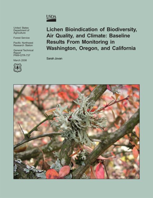
<strong>Lichen</strong> <strong>Bioindic<strong>at</strong>ion</strong> <strong>of</strong> <strong>Biodiversity</strong>,<br />
<strong>Air</strong> <strong>Quality</strong>, <strong>and</strong> Clim<strong>at</strong>e: Baseline<br />
Results From Monitoring in<br />
Washington, Oregon, <strong>and</strong> California<br />
Sarah Jovan
The Forest Service <strong>of</strong> the U.S. Department <strong>of</strong> Agriculture is dedic<strong>at</strong>ed to the<br />
principle <strong>of</strong> multiple use management <strong>of</strong> the N<strong>at</strong>ion’s forest resources for sustained<br />
yields <strong>of</strong> wood, w<strong>at</strong>er, forage, wildlife, <strong>and</strong> recre<strong>at</strong>ion. Through forestry<br />
research, cooper<strong>at</strong>ion with the St<strong>at</strong>es <strong>and</strong> priv<strong>at</strong>e forest owners, <strong>and</strong> management<br />
<strong>of</strong> the n<strong>at</strong>ional forests <strong>and</strong> n<strong>at</strong>ional grassl<strong>and</strong>s, it strives—as directed by<br />
Congress—to provide increasingly gre<strong>at</strong>er service to a growing N<strong>at</strong>ion.<br />
The U.S. Department <strong>of</strong> Agriculture (USDA) prohibits discrimin<strong>at</strong>ion in all its<br />
programs <strong>and</strong> activities on the basis <strong>of</strong> race, color, n<strong>at</strong>ional origin, age, disability,<br />
<strong>and</strong> where applicable, sex, marital st<strong>at</strong>us, familial st<strong>at</strong>us, parental st<strong>at</strong>us, religion,<br />
sexual orient<strong>at</strong>ion, genetic inform<strong>at</strong>ion, political beliefs, reprisal, or because all or<br />
part <strong>of</strong> an individual’s income is derived from any public assistance program. (Not<br />
all prohibited bases apply to all programs.) Persons with disabilities who require<br />
altern<strong>at</strong>ive means for communic<strong>at</strong>ion <strong>of</strong> program inform<strong>at</strong>ion (Braille, large print,<br />
audiotape, etc.) should contact USDA’s TARGET Center <strong>at</strong> (202) 720-2600 (voice<br />
<strong>and</strong> TDD).<br />
To file a complaint <strong>of</strong> discrimin<strong>at</strong>ion write USDA, Director, Office <strong>of</strong> Civil Rights,<br />
1400 Independence Avenue, S.W. Washington, DC 20250-9410, or call (800) 795-<br />
3272 (voice) or (202) 720-6382 (TDD). USDA is an equal opportunity provider <strong>and</strong><br />
employer.<br />
Author<br />
Sarah Jovan is a research lichenologist, Forestry Sciences Labor<strong>at</strong>ory,<br />
620 SW Main, Suite 400, Portl<strong>and</strong>, OR 97205.
Abstract<br />
Jovan, Sarah. 2008. <strong>Lichen</strong> bioindic<strong>at</strong>ion <strong>of</strong> biodiversity, air quality, <strong>and</strong> clim<strong>at</strong>e:<br />
baseline results from monitoring in Washington, Oregon, <strong>and</strong> California. Gen.<br />
Tech. Rep. PNW-GTR-737. Portl<strong>and</strong>, OR: U.S. Department <strong>of</strong> Agriculture,<br />
Forest Service, Pacific Northwest Research St<strong>at</strong>ion. 115 p.<br />
<strong>Lichen</strong>s are highly valued ecological indic<strong>at</strong>ors known for their sensitivity to a wide<br />
variety <strong>of</strong> environmental stressors like air quality <strong>and</strong> clim<strong>at</strong>e change. This report<br />
summarizes baseline results from the U.S. Department <strong>of</strong> Agriculture, Forest Service,<br />
Forest Inventory <strong>and</strong> Analysis (FIA) <strong>Lichen</strong> Community Indic<strong>at</strong>or covering<br />
the first full cycle <strong>of</strong> d<strong>at</strong>a collection (1998–2001, 2003) for Washington, Oregon,<br />
<strong>and</strong> California. During this period, FIA conducted 972 surveys <strong>of</strong> epiphytic<br />
macrolichen communities for monitoring both sp<strong>at</strong>ial <strong>and</strong> long-term temporal<br />
trends in forest health. Major research findings are presented with emphasis on<br />
lichen biodiversity as well as bioindic<strong>at</strong>ion <strong>of</strong> air quality <strong>and</strong> clim<strong>at</strong>e. Considerable<br />
effort is devoted to mapping geographic p<strong>at</strong>terns <strong>and</strong> defining lichen indic<strong>at</strong>or<br />
species suitable for estim<strong>at</strong>ing air quality <strong>and</strong> clim<strong>at</strong>e.<br />
Keywords: Acidophytes, air quality, California, clim<strong>at</strong>e change, cyanolichens,<br />
forest health, gradient analysis, indic<strong>at</strong>or species, neutrophytes, nitrophytes,<br />
nonmetric multidimensional scaling, ordin<strong>at</strong>ion, Pacific Northwest, pollution.
Contents<br />
Part I: The FIA <strong>Lichen</strong> Community Indic<strong>at</strong>or<br />
1 Chapter 1: Introduction <strong>and</strong> Methods<br />
1 Introduction<br />
4 <strong>Lichen</strong>s as Biological Indic<strong>at</strong>ors<br />
7 Report Objectives<br />
7 Methods<br />
10 <strong>Lichen</strong> Survey Protocol<br />
12 D<strong>at</strong>a Analysis Overview: Gradient Models Demystified<br />
Part II: <strong>Lichen</strong> Diversity Biomonitoring<br />
17 Chapter 2: Epiphytic <strong>Lichen</strong> Diversity <strong>and</strong> Forest Habit<strong>at</strong>s in<br />
Washington, Oregon, <strong>and</strong> California<br />
17 Key Findings<br />
17 Summary <strong>of</strong> <strong>Lichen</strong> Species Richness<br />
23 Coast Ranges<br />
23 Large Agricultural Valleys<br />
23 Cascade Range <strong>and</strong> Modoc Pl<strong>at</strong>eau<br />
25 Sierra Nevada<br />
25 Eastern Oregon <strong>and</strong> Washington<br />
27 Conclusions<br />
Part III: <strong>Air</strong> <strong>Quality</strong> Biomonitoring<br />
29 Chapter 3: <strong>Air</strong> <strong>Quality</strong> in the West-Side Pacific Northwest<br />
29 Key Findings<br />
29 Introduction to the Model<br />
32 Ancillary D<strong>at</strong>a: <strong>Lichen</strong> Nitrogen <strong>and</strong> Sulfur Content<br />
33 Interpret<strong>at</strong>ion <strong>of</strong> <strong>Air</strong> <strong>Quality</strong> Estim<strong>at</strong>es: Nitrogen Pollutants Are Key Stressors<br />
33 Discussion <strong>of</strong> Indic<strong>at</strong>or Species<br />
34 Direct <strong>and</strong> Indirect Nitrogen Effects on <strong>Lichen</strong>s<br />
34 Nitrophytes<br />
36 Acidophytes<br />
37 Neutrophytes<br />
38 Str<strong>at</strong>ified Cyanolichens<br />
39 Indic<strong>at</strong>or Synthesis
46 Summary <strong>of</strong> <strong>Air</strong> <strong>Quality</strong> P<strong>at</strong>terns<br />
50 Conclusions<br />
53 Chapter 4: <strong>Air</strong> <strong>Quality</strong> in the Gre<strong>at</strong>er Central Valley, California<br />
53 Key Findings<br />
53 Introduction to the Model<br />
55 Ancillary D<strong>at</strong>a: <strong>Air</strong> <strong>Quality</strong> Measurements<br />
56 Interpret<strong>at</strong>ion <strong>of</strong> <strong>Air</strong> <strong>Quality</strong> Estim<strong>at</strong>es: Nitrogen Is Shaping <strong>Lichen</strong><br />
Community Structure<br />
58 Discussion <strong>of</strong> Indic<strong>at</strong>or Species<br />
63 Summary <strong>of</strong> <strong>Air</strong> <strong>Quality</strong> P<strong>at</strong>terns<br />
65 Hotspots <strong>of</strong> Degraded <strong>Air</strong> <strong>Quality</strong><br />
67 Conclusions<br />
69 Chapter 5: <strong>Air</strong> <strong>Quality</strong> in the Gre<strong>at</strong>er Sierra Nevada, California<br />
69 Key Findings<br />
69 Introduction to the Model<br />
71 Model Adjustment for Elev<strong>at</strong>ion Effects<br />
72 Ancillary D<strong>at</strong>a: <strong>Lichen</strong> Nitrogen Content<br />
75 Interpret<strong>at</strong>ion <strong>of</strong> <strong>Air</strong> <strong>Quality</strong> Estim<strong>at</strong>es: Nitrogen Impacts Are Apparent<br />
75 Summary <strong>of</strong> <strong>Air</strong> <strong>Quality</strong> P<strong>at</strong>terns in the Gre<strong>at</strong>er Sierra Nevada<br />
76 Major Deposition P<strong>at</strong>terns<br />
79 Conclusions<br />
Part IV: Clim<strong>at</strong>e Mapping <strong>and</strong> Tracking<br />
81 Chapter 6: Clim<strong>at</strong>e Biomonitoring in the West-Side Pacific<br />
Northwest<br />
81 Key Findings<br />
81 Introduction to the Model<br />
81 Ancillary D<strong>at</strong>a: PRISM Model Clim<strong>at</strong>e D<strong>at</strong>a<br />
82 Interpret<strong>at</strong>ion <strong>of</strong> Clim<strong>at</strong>e Estim<strong>at</strong>es<br />
82 Review <strong>of</strong> Clim<strong>at</strong>e Zones <strong>and</strong> Indic<strong>at</strong>or Species From Geiser <strong>and</strong> Neitlich<br />
(2007)<br />
83 Large Str<strong>at</strong>ified Cyanolichens<br />
83 Hypermaritime Communities<br />
84 High-Elev<strong>at</strong>ion Communities<br />
86 Summary <strong>of</strong> Clim<strong>at</strong>e P<strong>at</strong>terns in the West-Side Pacific Northwest<br />
88 Conclusions
89 Chapter 7: Clim<strong>at</strong>e Biomonitoring in Northern <strong>and</strong> Central California<br />
89 Key Findings<br />
89 Introduction to the Model<br />
91 Ancillary D<strong>at</strong>a: PRISM Model Clim<strong>at</strong>e D<strong>at</strong>a<br />
91 Interpret<strong>at</strong>ion <strong>of</strong> Clim<strong>at</strong>e Estim<strong>at</strong>es<br />
91 Discussion <strong>of</strong> Clim<strong>at</strong>e Zones <strong>and</strong> Indic<strong>at</strong>or Species<br />
92 Proposed Temper<strong>at</strong>ure Effects<br />
96 Proposed Moisture Effects<br />
99 Summary <strong>of</strong> Clim<strong>at</strong>e P<strong>at</strong>terns in Northern <strong>and</strong> Central California<br />
99 Sp<strong>at</strong>ial Temper<strong>at</strong>ure P<strong>at</strong>terns<br />
99 Sp<strong>at</strong>ial Moisture P<strong>at</strong>terns<br />
101 Conclusions<br />
103 Chapter 8: Overall Conclusions<br />
104 Acknowledgments<br />
104 English Equivalents<br />
105 References
Part I: The FIA <strong>Lichen</strong> Community Indic<strong>at</strong>or<br />
Sticta fuliginosa (spotted felt lichen) found on Mount Hood N<strong>at</strong>ional Forest in Oregon.<br />
Roseann Barnhill
<strong>Lichen</strong> <strong>Bioindic<strong>at</strong>ion</strong> <strong>of</strong> <strong>Biodiversity</strong>, <strong>Air</strong> <strong>Quality</strong>, <strong>and</strong> Clim<strong>at</strong>e: Baseline Results From Monitoring...<br />
Chapter 1: Introduction <strong>and</strong> Methods<br />
Introduction<br />
Although appearing to be a single organism, a lichen (fig. 1) is actually a symbiotic<br />
partnership between a fungus <strong>and</strong> one or more photosynthetic organisms, an alga<br />
or cyanobacterium. Their intim<strong>at</strong>e coexistence inspired the analogy (originally<br />
conceived by Canadian lichenologist Trevor Goward) th<strong>at</strong> lichens are fungi th<strong>at</strong><br />
discovered agriculture (fig. 2). Typically the fungal partner provides most <strong>of</strong> the<br />
composite organism’s structure <strong>and</strong> mass, thus trading physical protection for<br />
carbohydr<strong>at</strong>es manufactured by the photosynthetic partner (fig. 3). Together the<br />
fungus <strong>and</strong> its partner(s) can inhabit a much wider variety <strong>of</strong> habit<strong>at</strong>s <strong>and</strong> conditions<br />
than any could on their own.<br />
The mountainous l<strong>and</strong>scapes <strong>of</strong> Washington, Oregon, <strong>and</strong> California support<br />
a very diverse <strong>and</strong> conspicuous lichen flora. This region is home to several rare,<br />
endemic, old-growth-associ<strong>at</strong>ed species such as Pseudocyphellaria rainierensis (fig.<br />
4) <strong>and</strong> Nephroma occultum (fig. 5) as well as species th<strong>at</strong> <strong>of</strong>ten achieve impressively<br />
high biomass in western forests, like Bryoria fremontii (fig. 6). <strong>Lichen</strong>s play<br />
many essential functional roles in these forested ecosystems. For instance, species<br />
<strong>of</strong> Bryoria <strong>and</strong> Alectoria are important forage for elk, caribou, deer, <strong>and</strong> flying<br />
squirrels (Maser et al. 1985, McCune 1993, Stevenson 1978). Birds, rodents, <strong>and</strong><br />
invertebr<strong>at</strong>es also use these pendulous, hair-like species for nesting m<strong>at</strong>erials <strong>and</strong><br />
shelter (Hayward <strong>and</strong> Rosentreter 1994, Pettersson et al. 1995).<br />
<strong>Lichen</strong>s play many<br />
essential functional<br />
roles in these forested<br />
ecosystems.<br />
Figure 1—Hypogymnia physodes (tube lichen), one <strong>of</strong> several<br />
Hypogymnia species occurring in the Pacific Western St<strong>at</strong>es.<br />
Sarah Jovan<br />
1
GENERAL TECHNICAL REPORT PNW-GTR-737<br />
Figure 2—Lobaria pulmonaria (lung lichen), a large species found in wet forests <strong>of</strong><br />
the Pacific Northwest.<br />
Daphne Stone<br />
Figure 3—Cross section <strong>of</strong> the lichen Lobaria pulmonaria, a three-way symbiosis between a<br />
fungus, algae, <strong>and</strong> cyanobacteria. Fungal cells are loc<strong>at</strong>ed in the upper cortex (UC), medulla<br />
(M), <strong>and</strong> lower cortex (LC). Photosynthesis occurs in the green algal layer (A) <strong>and</strong> nodules<br />
containing cyanobacteria (CB). The cyanobacteria also fix <strong>at</strong>mospheric nitrogen into a form<br />
th<strong>at</strong> is useable to plants.<br />
Eric Peterson from www.crustose.net<br />
2
<strong>Lichen</strong> <strong>Bioindic<strong>at</strong>ion</strong> <strong>of</strong> <strong>Biodiversity</strong>, <strong>Air</strong> <strong>Quality</strong>, <strong>and</strong> Clim<strong>at</strong>e: Baseline Results From Monitoring...<br />
Jim Riley<br />
Figure 4—Pseudocyphellaria rainierensis<br />
(Rainier pseudocyphellaria lichen). Provided<br />
courtesy <strong>of</strong> OSU <strong>Lichen</strong> Group. 1999. Photographs<br />
<strong>of</strong> Pacific Northwest <strong>Lichen</strong>s. Oregon<br />
St<strong>at</strong>e University, Department <strong>of</strong> Botany <strong>and</strong><br />
Plant P<strong>at</strong>hology, <strong>Lichen</strong> Research Group.<br />
Figure 5—Nephroma occultum (kidney lichen), a rare lichen species inhabiting<br />
old-growth forests in the Pacific Northwest.<br />
Tim Wheeler<br />
3
GENERAL TECHNICAL REPORT PNW-GTR-737<br />
Figure 6—Conifers laden with Bryoria fremontii (Freemont’s horsehair lichen) in Starkey<br />
Experimental Forest, eastern Oregon.<br />
Sarah Jovan<br />
Cyanolichens such as Pseudocyphellaria anthraspis, P. croc<strong>at</strong>a (fig. 7), <strong>and</strong><br />
Lobaria oregana (fig. 8) make important contributions to nutrient cycling in Pacific<br />
Northwest forests as their cyanobacteria partners fix <strong>at</strong>mospheric nitrogen (N 2<br />
) into<br />
a form th<strong>at</strong> is useable by plants. Nitrogen inputs from cyanolichens may be quite<br />
substantial, especially in moist, old-growth forests. It is estim<strong>at</strong>ed th<strong>at</strong> L. oregana<br />
alone fixes as much as 16.5 kg N -1·yr 2·ha -1 <strong>at</strong> some high biomass sites in the western<br />
Cascades <strong>of</strong> Oregon (Antoine 2004). These lichens, like many others, are critical<br />
components <strong>of</strong> western ecosystems <strong>and</strong> directly influence forest health.<br />
<strong>Lichen</strong>s as Biological Indic<strong>at</strong>ors<br />
<strong>Lichen</strong>s are <strong>of</strong>ten likened to canaries in a coal mine because some species are<br />
extremely sensitive to environmental change, a major reason for their popularity as<br />
bioindic<strong>at</strong>ors for n<strong>at</strong>ural resource assessment (e.g., Nimis et al. 2002). The Forest<br />
Inventory <strong>and</strong> Analysis (FIA) Program <strong>of</strong> the U.S. Department <strong>of</strong> Agriculture,<br />
Forest Service (USFS), includes lichens among a suite <strong>of</strong> forest health indic<strong>at</strong>ors<br />
(Stolte et al. 2002) th<strong>at</strong> are monitored n<strong>at</strong>ionwide on a permanent sampling grid<br />
(Will-Wolf 2005). Formally known as the FIA <strong>Lichen</strong> Community Indic<strong>at</strong>or, these<br />
4
<strong>Lichen</strong> <strong>Bioindic<strong>at</strong>ion</strong> <strong>of</strong> <strong>Biodiversity</strong>, <strong>Air</strong> <strong>Quality</strong>, <strong>and</strong> Clim<strong>at</strong>e: Baseline Results From Monitoring...<br />
Tim Wheeler<br />
Figure 7—Pseudocyphellaria croc<strong>at</strong>a (Pseudocyphellaria lichen); its bright<br />
yellow soredia (powdery clusters <strong>of</strong> algal cells <strong>and</strong> fungal str<strong>and</strong>s erupting<br />
from the surface) are diagnostic.<br />
Eric Straley<br />
Figure 8—Lobaria oregana<br />
(Oregon lung lichen), an<br />
important nitrogen-fixer in<br />
western forests.<br />
d<strong>at</strong>a are periodic surveys <strong>of</strong> epiphytic (“tree-dwelling”) lichen communities conducted<br />
by specially trained field crews (fig. 9).<br />
The structure <strong>of</strong> a lichen community in a forest (i.e., species presence <strong>and</strong><br />
abundance) intrinsically provides a wealth <strong>of</strong> inform<strong>at</strong>ion about forest health, function,<br />
<strong>and</strong> local clim<strong>at</strong>ic conditions (fig. 10). Analysts can extract particular properties<br />
<strong>of</strong> the community d<strong>at</strong>a, such as indices <strong>of</strong> indic<strong>at</strong>or species <strong>and</strong> community<br />
gradients, to address a wide variety <strong>of</strong> monitoring questions (See sidebar 1).<br />
At present, the three primary objectives <strong>of</strong> the <strong>Lichen</strong> Community Indic<strong>at</strong>or are to<br />
The structure <strong>of</strong> a<br />
lichen community in<br />
a forest intrinsically<br />
provides a wealth<br />
<strong>of</strong> inform<strong>at</strong>ion about<br />
forest health, function,<br />
<strong>and</strong> local<br />
clim<strong>at</strong>ic conditions.<br />
5
GENERAL TECHNICAL REPORT PNW-GTR-737<br />
Figure 9—The Alaskan Forest Inventory <strong>and</strong> Analysis crew<br />
training for the 2006 lichen certific<strong>at</strong>ion exam. This was the<br />
second year <strong>of</strong> lichen surveying in coastal Alaska.<br />
Sarah Jovan<br />
Figure 10—Concept behind the <strong>Lichen</strong> Community Indic<strong>at</strong>or. N = nitrogen, S = sulfur.<br />
6
<strong>Lichen</strong> <strong>Bioindic<strong>at</strong>ion</strong> <strong>of</strong> <strong>Biodiversity</strong>, <strong>Air</strong> <strong>Quality</strong>, <strong>and</strong> Clim<strong>at</strong>e: Baseline Results From Monitoring...<br />
Sidebar 1: Why use bioindic<strong>at</strong>ors?<br />
Wh<strong>at</strong> is the r<strong>at</strong>ionale for biomonitoring when we are technologically capable<br />
<strong>of</strong> directly measuring forest conditions? Perhaps the most immedi<strong>at</strong>e benefit<br />
is the ability to map conditions <strong>at</strong> a sampling intensity th<strong>at</strong> is prohibitively<br />
expensive with active monitors. Moreover, bioindic<strong>at</strong>ors are intim<strong>at</strong>ely tied to<br />
local conditions. Their responses to stressors are <strong>of</strong>ten more represent<strong>at</strong>ive <strong>of</strong><br />
cumul<strong>at</strong>ive impact on the function <strong>and</strong> diversity <strong>of</strong> the surrounding ecosystem<br />
than are active monitors.<br />
evalu<strong>at</strong>e <strong>and</strong> monitor biodiversity, air quality, <strong>and</strong> clim<strong>at</strong>e. Survey d<strong>at</strong>a may be<br />
directly applied for biodiversity monitoring, whereas the l<strong>at</strong>ter two applic<strong>at</strong>ions<br />
involve multivari<strong>at</strong>e gradient models.<br />
Report Objectives<br />
Four gradient models th<strong>at</strong> use FIA lichen d<strong>at</strong>a to estim<strong>at</strong>e air quality <strong>and</strong> clim<strong>at</strong>e<br />
have been implemented in the study region, <strong>and</strong> three to four additional models<br />
are scheduled for completion within the next few years (fig. 11 <strong>and</strong> table 1). The<br />
main objective <strong>of</strong> this report is to summarize lichen biodiversity <strong>and</strong> major research<br />
findings from the four completed gradient models. Summaries typically include<br />
both original analysis <strong>and</strong> review <strong>of</strong> previously published articles. <strong>Air</strong> quality<br />
results are mapped to indic<strong>at</strong>e forests <strong>at</strong> gre<strong>at</strong>est risk <strong>of</strong> ecological degrad<strong>at</strong>ion,<br />
<strong>and</strong> modeled clim<strong>at</strong>e estim<strong>at</strong>es likewise signify current conditions affecting forests.<br />
<strong>Lichen</strong> indic<strong>at</strong>or species are examined to help link air quality estim<strong>at</strong>es to<br />
specific pollutants <strong>and</strong> also to illustr<strong>at</strong>e the biological underpinnings <strong>of</strong> each<br />
gradient model. These baseline results are <strong>of</strong> gre<strong>at</strong> interest to forest <strong>and</strong> air managers,<br />
serving as the first large-scale comprehensive assessments <strong>of</strong> forest health for<br />
the study region.<br />
These baseline<br />
results are <strong>of</strong> gre<strong>at</strong><br />
interest to forest<br />
<strong>and</strong> air managers,<br />
serving as the first<br />
large-scale comprehensive<br />
assessments<br />
<strong>of</strong> forest<br />
health for the study<br />
region.<br />
Methods<br />
This section covers the survey protocol for the <strong>Lichen</strong> Community Indic<strong>at</strong>or<br />
(USDA FS 2005) as well as analytical methods used to build gradient models for<br />
air quality <strong>and</strong> clim<strong>at</strong>e bioindic<strong>at</strong>ion. These general overviews are critical to underst<strong>and</strong>ing<br />
the basis for results presented in the following chapters. Less essential but<br />
more technical explan<strong>at</strong>ions are presented in sidebars. Any model-specific methods<br />
are described in their respective chapters.<br />
7
GENERAL TECHNICAL REPORT PNW-GTR-737<br />
Figure 11—Map <strong>of</strong> all sites in Washington, Oregon, <strong>and</strong> California surveyed for lichen communities. Plots are grouped in<br />
model areas as described in table 1. Federal class 1 areas are shown because they receive special air quality protection<br />
under the Clean <strong>Air</strong> Act (Section 162(a)). These include n<strong>at</strong>ional parks, n<strong>at</strong>ional wilderness areas, <strong>and</strong> n<strong>at</strong>ional monuments.<br />
Plot loc<strong>at</strong>ions are approxim<strong>at</strong>e.<br />
8
Table 1—Implement<strong>at</strong>ion <strong>of</strong> the Forest Inventory <strong>and</strong> Analysis <strong>Lichen</strong> Indic<strong>at</strong>or in Washington, Oregon, <strong>and</strong> California a<br />
Estim<strong>at</strong>ed Anticip<strong>at</strong>ed<br />
Model region parameters Progress Cit<strong>at</strong>ion completion Notes<br />
Pacific Northwest, west-side <strong>Air</strong> quality, clim<strong>at</strong>e Complete Geiser <strong>and</strong> Neitlich 2007 Done See chapters 3 <strong>and</strong> 6<br />
Pacific Northwest, east-side <strong>Air</strong> quality, clim<strong>at</strong>e In progress Fall 2007 May include plots from Montana <strong>and</strong> Idaho<br />
California, Northwest Coast <strong>Air</strong> quality In progress Summer 2007 Region may be merged with the west-side Pacific<br />
Northwest Model<br />
California, Gre<strong>at</strong>er Central Valley <strong>Air</strong> quality Complete Jovan <strong>and</strong> McCune 2005 Done See chapter 4<br />
California, Gre<strong>at</strong>er Sierra Nevada <strong>Air</strong> quality Complete Jovan <strong>and</strong> McCune 2006 Done See chapter 5<br />
<strong>Lichen</strong> <strong>Bioindic<strong>at</strong>ion</strong> <strong>of</strong> <strong>Biodiversity</strong>, <strong>Air</strong> <strong>Quality</strong>, <strong>and</strong> Clim<strong>at</strong>e: Baseline Results From Monitoring...<br />
California, Northern <strong>and</strong> Central Clim<strong>at</strong>e Complete Jovan <strong>and</strong> McCune 2004 Done Encompasses gre<strong>at</strong>er Central Valley, gre<strong>at</strong>er Sierra<br />
Nevada, <strong>and</strong> Northwest coast models; See chapter 7<br />
California, Gre<strong>at</strong>er Los Angeles<br />
Basin <strong>Air</strong> quality, clim<strong>at</strong>e Study plan under 2008 or 2009 Model boundaries in figure 11 are preliminary<br />
development<br />
California, Southeast Desert<br />
Basin <strong>and</strong> Range <strong>Air</strong> quality, clim<strong>at</strong>e Study plan in Not yet May be merged with a model for the Southwest<br />
discussion scheduled (Arizona, New Mexico, <strong>and</strong> Nevada)<br />
Model boundaries are shown in figure 11.<br />
a<br />
9
GENERAL TECHNICAL REPORT PNW-GTR-737<br />
The FIA crews have<br />
completed lichen<br />
surveys <strong>at</strong> a full<br />
cycle <strong>of</strong> plots for<br />
California <strong>and</strong><br />
Oregon <strong>and</strong><br />
Washington.<br />
The FIA crews have completed lichen surveys <strong>at</strong> a full cycle <strong>of</strong> plots for Forest<br />
Service Regions 5 (California) <strong>and</strong> 6 (Oregon <strong>and</strong> Washington; fig. 11). Five<br />
panels <strong>of</strong> plots were surveyed in 1998, 1999, 2000, 2001, <strong>and</strong> 2003, <strong>and</strong> resurveys<br />
are tent<strong>at</strong>ively scheduled to begin in 2010. Extensive measurements <strong>of</strong> forest st<strong>and</strong><br />
structure, history, <strong>and</strong> productivity are system<strong>at</strong>ically collected n<strong>at</strong>ionwide <strong>at</strong> one<br />
plot for every 2430 ha on the FIA phase 2 (P2) grid. Every 16 th plot is also a phase<br />
3 (P3) plot where additional d<strong>at</strong>a are collected for all Forest Health Indic<strong>at</strong>ors,<br />
which includes the <strong>Lichen</strong> Community Indic<strong>at</strong>or (Stolte et al. 2002).<br />
<strong>Lichen</strong> Survey Protocol<br />
<strong>Lichen</strong> community surveys are conducted on a circular, 0.378-ha plot centered<br />
on subplot 1 in the st<strong>and</strong>ard FIA plot design (fig. 12). Surveys last a minimum<br />
<strong>of</strong> 30 minutes <strong>and</strong> a maximum <strong>of</strong> 2 hours during which the crew member collects<br />
a voucher specimen <strong>of</strong> every epiphytic macrolichen species encountered. Although<br />
d<strong>at</strong>a are not a complete inventory <strong>of</strong> all macrolichen species on a plot, this costeffective<br />
survey protocol gener<strong>at</strong>es represent<strong>at</strong>ive <strong>and</strong> repe<strong>at</strong>able plot d<strong>at</strong>a th<strong>at</strong> are<br />
comparable across the country. Abundance is estim<strong>at</strong>ed for each species by using<br />
broad abundance codes (table 2). Surveyors collect from the surface <strong>of</strong> all st<strong>and</strong>ing<br />
woody substr<strong>at</strong>es, above 0.5 m <strong>and</strong> within arm’s reach, <strong>and</strong> also freshly fallen<br />
lichens in the litter. Vouchers are sent to pr<strong>of</strong>essional lichenologists for identific<strong>at</strong>ion<br />
in the lab.<br />
Figure 12—Forest Inventory <strong>and</strong> Analysis plot design. <strong>Lichen</strong> communities<br />
are surveyed in the shaded area.<br />
10
<strong>Lichen</strong> <strong>Bioindic<strong>at</strong>ion</strong> <strong>of</strong> <strong>Biodiversity</strong>, <strong>Air</strong> <strong>Quality</strong>, <strong>and</strong> Clim<strong>at</strong>e: Baseline Results From Monitoring...<br />
Table 2—Abundance codes used during lichen community surveys<br />
Code<br />
Abundance<br />
1 Infrequent (1 to 3 thalli)<br />
2 Uncommon (4 to 10 thalli)<br />
3 Common (>10 thalli; species occurring on less than 50 percent <strong>of</strong> all boles<br />
<strong>and</strong> branches in plot)<br />
4 Abundant (>10 thalli; species occurring on gre<strong>at</strong>er than 50 percent <strong>of</strong> boles<br />
<strong>and</strong> branches in the plot)<br />
Surveyors are nonspecialists specially trained to differenti<strong>at</strong>e between lichen<br />
species. Every year surveyors must pass a certific<strong>at</strong>ion exam administered by a<br />
pr<strong>of</strong>essional lichenologist (fig. 13). At a practice FIA plot, the number <strong>of</strong> species<br />
the trainee collects must be 65 percent or more <strong>of</strong> the number found by the<br />
lichenologist in order to certify. The lichenologist then periodically audits crews<br />
during the field season with hot <strong>and</strong> blind checks to ensure th<strong>at</strong> species capture<br />
continues to meet the 65 percent measurement tolerance. Hot checks are mainly<br />
instructive, where crew members <strong>and</strong> the lichenologist survey a plot simultaneously.<br />
Blind-checked plots are usually surveyed by a lichenologist within 1<br />
month <strong>of</strong> the crew, without knowledge <strong>of</strong> the crew’s d<strong>at</strong>a, <strong>and</strong> provide a measure<br />
<strong>of</strong> d<strong>at</strong>a quality. <strong>Air</strong> quality estim<strong>at</strong>es from FIA gradient models have been found<br />
to be highly repe<strong>at</strong>able as long as the 65 percent criterion is met (McCune et al.<br />
1997).<br />
Figure 13—The Alaskan Forest Inventory <strong>and</strong> Analysis crew<br />
prepares for the 2006 lichen certific<strong>at</strong>ion exam.<br />
Sarah Jovan<br />
11
GENERAL TECHNICAL REPORT PNW-GTR-737<br />
To help build gradient models for air quality or clim<strong>at</strong>e bioindic<strong>at</strong>ion, additional<br />
lichen surveys may be conducted <strong>at</strong> temporary plots <strong>of</strong>f the regular FIA<br />
grid (i.e., <strong>of</strong>f-frame plots). These plots are str<strong>at</strong>egically loc<strong>at</strong>ed in areas <strong>of</strong> special<br />
interest or significance (e.g., wilderness areas <strong>and</strong> n<strong>at</strong>ional parks) or in places expected<br />
to be highly polluted (e.g., in cities, near industry) in order to capture the<br />
entire regional pollution gradient. Off-frame plots are <strong>of</strong>ten co-loc<strong>at</strong>ed with air<br />
quality monitors.<br />
D<strong>at</strong>a Analysis Overview: Gradient Models Demystified<br />
Usually <strong>at</strong> least two<br />
strong gradients<br />
can be extracted<br />
from the FIA lichen<br />
d<strong>at</strong>a: one gradient<br />
in community composition<br />
rel<strong>at</strong>ing<br />
to air quality <strong>and</strong><br />
a second gradient<br />
rel<strong>at</strong>ing to<br />
macroclim<strong>at</strong>e.<br />
A model built with gradient analysis (see McCune <strong>and</strong> Grace 2002) is required to<br />
apply the lichen community d<strong>at</strong>a for air quality <strong>and</strong> clim<strong>at</strong>e monitoring. Gradient<br />
analysis helps the investig<strong>at</strong>or detect the strongest p<strong>at</strong>terns (i.e., gradients) in lichen<br />
community composition <strong>and</strong> determine how they rel<strong>at</strong>e to environmental variables.<br />
Gradient models are typically developed by using either nonmetric multidimensional<br />
scaling ordin<strong>at</strong>ion (NMS) (Kruskal 1964) or regression techniques (or some<br />
combin<strong>at</strong>ion <strong>of</strong> the two). Usually <strong>at</strong> least two strong gradients can be extracted<br />
from the FIA lichen d<strong>at</strong>a: one gradient in community composition rel<strong>at</strong>ing to air<br />
quality <strong>and</strong> a second gradient rel<strong>at</strong>ing to macroclim<strong>at</strong>e.<br />
Analysts tailor these gradient models to meet the management objectives <strong>and</strong><br />
research needs <strong>of</strong> their respective coverage areas. Thus no two models are exactly<br />
alike. Attempts are made to integr<strong>at</strong>e lichen d<strong>at</strong>a with outside sources <strong>of</strong> inform<strong>at</strong>ion,<br />
such as measurements <strong>of</strong> pollutant concentr<strong>at</strong>ions or deposition <strong>at</strong> <strong>of</strong>f-frame<br />
plots, modeled clim<strong>at</strong>e estim<strong>at</strong>es, <strong>and</strong> FIA forest mensur<strong>at</strong>ion d<strong>at</strong>a collected from<br />
the P2 <strong>and</strong> P3 grids, as well as lichen survey d<strong>at</strong>a from other l<strong>and</strong>scape-scale<br />
sampling grids.<br />
Nonmetric multidimensional scaling—<br />
Nonmetric multidimensional scaling is a powerful tool for gradient analysis <strong>of</strong><br />
complex ecological d<strong>at</strong>a (McCune <strong>and</strong> Grace 2002) <strong>and</strong> provides the found<strong>at</strong>ion<br />
for three <strong>of</strong> the four models discussed in this report. Basically NMS simultaneously<br />
considers the abundance <strong>of</strong> all lichen species in all plots by using a “distance measure”<br />
(e.g., Sørensen or Euclidean distance; McCune <strong>and</strong> Grace 2002). This measure<br />
is a m<strong>at</strong>hem<strong>at</strong>ical expression th<strong>at</strong> quantifies how community composition<br />
differs between each <strong>and</strong> every plot in the d<strong>at</strong>a. NMS uses these differences to<br />
12
<strong>Lichen</strong> <strong>Bioindic<strong>at</strong>ion</strong> <strong>of</strong> <strong>Biodiversity</strong>, <strong>Air</strong> <strong>Quality</strong>, <strong>and</strong> Clim<strong>at</strong>e: Baseline Results From Monitoring...<br />
detect gradients in community composition <strong>and</strong> score plots along them (see sidebar<br />
2). All reported NMS analyses were conducted using the PC-ORD s<strong>of</strong>tware package<br />
1 (McCune <strong>and</strong> Mefford 1999).<br />
Tools including sc<strong>at</strong>terplots, regression, <strong>and</strong> overlays are used to determine<br />
how these lichen community gradients rel<strong>at</strong>e to environmental factors. For example,<br />
if a gradient detected by NMS is strongly correl<strong>at</strong>ed with pollution variables<br />
(e.g., nitrogen deposition or sulfur dioxide concentr<strong>at</strong>ion), the score <strong>of</strong> a plot<br />
on th<strong>at</strong> gradient serves as a rel<strong>at</strong>ive estim<strong>at</strong>e <strong>of</strong> local air quality. The FIA lichen<br />
surveys contain an enormous amount <strong>of</strong> inform<strong>at</strong>ion as lichens respond to many<br />
Sidebar 2: Technical aspects <strong>of</strong> nonmetric multidimensional<br />
scaling (NMS)<br />
The d<strong>at</strong>a set used to build an NMS model with PC-ORD (McCune <strong>and</strong><br />
Mefford 1999) is an n x p m<strong>at</strong>rix <strong>of</strong> Forest Inventory <strong>and</strong> Analysis plots<br />
(rows) by species (columns), with each cell containing a lichen abundance<br />
code (table 2). NMS is indirect ordin<strong>at</strong>ion, meaning th<strong>at</strong> detected gradients<br />
are based solely on the ecological inform<strong>at</strong>ion given by the distributions <strong>of</strong><br />
species among plots. This process is technically a transform<strong>at</strong>ion <strong>of</strong> the plots<br />
as points in p-dimensional species space to a lower dimensional space, which<br />
is accomplished through hundreds <strong>of</strong> iter<strong>at</strong>ions. Each detected gradient is,<br />
functionally, an independent response <strong>of</strong> lichen communities to one or more<br />
environmental conditions (i.e., an environmental gradient). The analyst must<br />
discover the identity <strong>of</strong> these environmental conditions by looking <strong>at</strong> ancillary<br />
environmental d<strong>at</strong>a.<br />
Because NMS gener<strong>at</strong>es major community gradients without consider<strong>at</strong>ion<br />
<strong>of</strong> environmental variables (unlike the other popular techniques, canonical<br />
correspondence analysis <strong>and</strong> redundancy analysis) (Økl<strong>and</strong> 1996), it is<br />
st<strong>at</strong>istically valid to correl<strong>at</strong>e environmental variables with community<br />
gradients to make predictions. It is also st<strong>at</strong>istically valid to make predictions<br />
for new plots, which can be easily fit to the NMS axes. For further technical<br />
detail, an excellent introduction to NMS is given by McCune <strong>and</strong> Grace<br />
(2002, chapter 16).<br />
1<br />
Use <strong>of</strong> trade <strong>of</strong> firm names in this public<strong>at</strong>ion is for inform<strong>at</strong>ion <strong>and</strong> does not imply<br />
endorsement <strong>of</strong> any product or service by the U.S. Department <strong>of</strong> Agriculture.<br />
13
GENERAL TECHNICAL REPORT PNW-GTR-737<br />
Once community<br />
gradients are linked<br />
to the environmental<br />
gradient(s) they<br />
reflect, indic<strong>at</strong>or<br />
species for th<strong>at</strong><br />
environmental<br />
factor can be<br />
identified.<br />
aspects <strong>of</strong> their local environment. In essence, NMS is a distill<strong>at</strong>ion <strong>of</strong> th<strong>at</strong> inform<strong>at</strong>ion<br />
into the strongest p<strong>at</strong>terns. Once community gradients are linked to the<br />
environmental gradient(s) they reflect, indic<strong>at</strong>or species for th<strong>at</strong> environmental<br />
factor can be identified.<br />
Identifying indic<strong>at</strong>or species with species scores—<br />
Species scores were used in chapters 3 <strong>and</strong> 4 to identify pollution indic<strong>at</strong>or species.<br />
Basically each species used to build an NMS model is scored on each <strong>of</strong> the detected<br />
lichen community gradients. The calcul<strong>at</strong>ion involves simple weighted averaging<br />
th<strong>at</strong> considers how the species’ abundance was distributed among plots <strong>and</strong> how<br />
those plots scored on the gradient. The species’ score is technically its average position<br />
on the gradient <strong>and</strong> a represent<strong>at</strong>ion <strong>of</strong> the species’ optimum (i.e., for air<br />
Sidebar 3: Calcul<strong>at</strong>ing species scores<br />
Species scores are calcul<strong>at</strong>ed by using PC-ORD (McCune <strong>and</strong> Mefford 1999)<br />
in a single weighted-averaging step, whereby species abundance is weighted<br />
by plot scores from the nonmetric multidimensional scale air quality gradient:<br />
v<br />
n<br />
∑aijwi<br />
i=<br />
1<br />
=<br />
j n<br />
∑a<br />
i=<br />
1<br />
ij<br />
where v j<br />
= score for species j, a ij<br />
= abundance <strong>of</strong> species j in plot i, w i<br />
is<br />
the plot score <strong>of</strong> plot i, <strong>and</strong> n is the number <strong>of</strong> species on the plot. A few<br />
important cave<strong>at</strong>s are (1) scores for infrequent species are based on less d<strong>at</strong>a<br />
<strong>and</strong> so their scores are less reliable, (2) this analysis is susceptible to bias <strong>at</strong><br />
extremes <strong>of</strong> the air quality gradient as species scores are restricted to the range<br />
<strong>of</strong> the d<strong>at</strong>a even if the species’ true optimum lies beyond the d<strong>at</strong>a extremes<br />
(McCune <strong>and</strong> Grace 2002), <strong>and</strong> (3) a score can be calcul<strong>at</strong>ed for every species<br />
even if the species does not actually respond to air quality. Species scores<br />
suggest pollution sensitivity or intolerance but should be supported by multiple<br />
lines <strong>of</strong> evidence.<br />
14
<strong>Lichen</strong> <strong>Bioindic<strong>at</strong>ion</strong> <strong>of</strong> <strong>Biodiversity</strong>, <strong>Air</strong> <strong>Quality</strong>, <strong>and</strong> Clim<strong>at</strong>e: Baseline Results From Monitoring...<br />
quality or clim<strong>at</strong>e) (McCune <strong>and</strong> Grace 2002). For a gradient linked to air quality,<br />
species scores serve as rough estim<strong>at</strong>es <strong>of</strong> how species respond individually to<br />
pollution in the study area, given a few cave<strong>at</strong>s (see sidebar 3). Species are scored<br />
along the same gradient as plots. This means th<strong>at</strong> any c<strong>at</strong>egoriz<strong>at</strong>ion <strong>of</strong> air quality<br />
scores th<strong>at</strong> the analyst uses to summarize plots (e.g., best, fair, worst) can be used<br />
to gauge the implic<strong>at</strong>ions <strong>of</strong> species scores <strong>and</strong> vice versa.<br />
Indic<strong>at</strong>or species analysis—<br />
A second tool for identific<strong>at</strong>ion <strong>of</strong> indic<strong>at</strong>or species, Indic<strong>at</strong>or Species Analysis<br />
(ISA) (Dufrêne <strong>and</strong> Legendre 1997), is used in chapters 3, 6, <strong>and</strong> 7 to determine<br />
air quality <strong>and</strong> clim<strong>at</strong>e indic<strong>at</strong>ors. The ISA is a nonparametric analysis available in<br />
PC-ORD (McCune <strong>and</strong> Mefford 1999) th<strong>at</strong> evalu<strong>at</strong>es the faithfulness <strong>and</strong> exclusivity<br />
<strong>of</strong> each species to predefined groups <strong>of</strong> plots (McCune <strong>and</strong> Grace 2002), which are<br />
both fundamental characteristics <strong>of</strong> a reliable indic<strong>at</strong>or. The analyst chooses how to<br />
best divide plots into a priori groups, which <strong>of</strong>ten involves segment<strong>at</strong>ion <strong>of</strong> the air<br />
quality or clim<strong>at</strong>e gradient into useful c<strong>at</strong>egories (e.g., low, medium, <strong>and</strong> high pollution).<br />
To assess st<strong>at</strong>istical significance <strong>of</strong> indic<strong>at</strong>or species, a r<strong>and</strong>omiz<strong>at</strong>ion test is<br />
used whereby plots are r<strong>and</strong>omly reassigned to the groups 1,000 times (McCune <strong>and</strong><br />
Grace 2002).<br />
15
GENERAL TECHNICAL REPORT PNW-GTR-737<br />
Part II: <strong>Lichen</strong> Diversity Biomonitoring<br />
Evalu<strong>at</strong>ion <strong>of</strong> lichen species richness (i.e., a count <strong>of</strong> species encountered) is the<br />
main, formalized applic<strong>at</strong>ion <strong>of</strong> the Forest Inventory <strong>and</strong> Analysis (FIA), U.S.<br />
Department <strong>of</strong> Agriculture, Forest Service, <strong>Lichen</strong> Community Indic<strong>at</strong>or in regions<br />
awaiting air quality <strong>and</strong> clim<strong>at</strong>e bioindic<strong>at</strong>ion models. Because lichen surveys are<br />
timed, these species counts are technically a richness index r<strong>at</strong>her than an unbiased<br />
estim<strong>at</strong>or for plot species richness. <strong>Lichen</strong> diversity is commonly used as a general<br />
indic<strong>at</strong>or <strong>of</strong> forest health <strong>and</strong> “ecological function” (Will-Wolf et al. 2002), as<br />
lichens are key primary producers with important linkages to nutrient cycling <strong>and</strong><br />
forest food webs (see chapter 1 “Introduction”). High or low lichen diversity can<br />
result from certain types <strong>of</strong> air pollution, changes to forest management or st<strong>and</strong><br />
structure, diversity <strong>of</strong> plant substr<strong>at</strong>es available for coloniz<strong>at</strong>ion, favorability <strong>of</strong><br />
clim<strong>at</strong>e, return interval <strong>of</strong> disturbances like fire, <strong>and</strong> so on. As such, species richness<br />
is a simple parameter with a complex origin <strong>and</strong> interpret<strong>at</strong>ion. To answer<br />
more specific questions about the local forest environment, analysts <strong>of</strong>ten parse out<br />
richness indices by using lichen indic<strong>at</strong>or species. Richness or abundance <strong>of</strong> pollution<br />
indic<strong>at</strong>ors, for instance, is commonly used in the FIA lichen-air quality models<br />
(see chapters 3 to 5).<br />
Sarah Jovan<br />
Over 20 species <strong>of</strong> lichens inhabit this small oak in Walnut Park, Corvallis, Oregon.<br />
16
<strong>Lichen</strong> <strong>Bioindic<strong>at</strong>ion</strong> <strong>of</strong> <strong>Biodiversity</strong>, <strong>Air</strong> <strong>Quality</strong>, <strong>and</strong> Clim<strong>at</strong>e: Baseline Results From Monitoring...<br />
Chapter 2: Epiphytic <strong>Lichen</strong> Diversity <strong>and</strong><br />
Forest Habit<strong>at</strong>s in Washington, Oregon,<br />
<strong>and</strong> California<br />
Key Findings<br />
1. In total, 263 epiphytic lichen species were found among 779 plots<br />
2. Zero to 45 species occurred per plot. Plot-level species richness was highly<br />
heterogeneous within most ecoregions.<br />
3. Prominent hotspots <strong>of</strong> diversity include the Klam<strong>at</strong>h-Siskiyou region shared by<br />
Oregon <strong>and</strong> California, the Oregon-side western Cascades, <strong>and</strong> the Washingtonside<br />
eastern Cascades.<br />
4. Highest diversity was found in the Okanogan highl<strong>and</strong>s <strong>of</strong> eastern Washington,<br />
where plots supported an average richness <strong>of</strong> 21.8 species. The eastern Blue<br />
Mountains farther south likewise supported a considerable density <strong>of</strong> speciesrich<br />
plots.<br />
5. Plots were sparsely distributed over dry, shrubby ecoregions th<strong>at</strong> lack substantial<br />
forest cover like the Columbia Basin, Northwestern Basin <strong>and</strong> Range, Owyhee<br />
upl<strong>and</strong>s, <strong>and</strong> the agricultural Central Valley. Species richness estim<strong>at</strong>es are least<br />
reliable from these poorly sampled areas.<br />
Summary <strong>of</strong> <strong>Lichen</strong> Species Richness<br />
Washington, Oregon, <strong>and</strong> California are home to a wide array <strong>of</strong> forested ecosystems<br />
(fig. 14, table 3). The terrain is highly mountainous <strong>and</strong> along these steep<br />
elev<strong>at</strong>ion gradients, clim<strong>at</strong>e <strong>and</strong> forest composition change drastically (fig. 15). The<br />
diversity <strong>of</strong> conditions is reflected by a remarkable diversity <strong>of</strong> lichens (fig. 16).<br />
An impressive total <strong>of</strong> 263 epiphytic lichen species were found in the region from a<br />
full cycle <strong>of</strong> survey d<strong>at</strong>a (n = 779, 1998-2001, 2003) collected by the Forest Inventory<br />
<strong>and</strong> Analysis (FIA) Program, U.S. Department <strong>of</strong> Agriculture. Among all<br />
plots surveyed in Washington (n = 199), Oregon (n = 292), <strong>and</strong> California (n =<br />
288), plot-level species richness ranged from 0 to 45 species (tables 4 <strong>and</strong> 5). The<br />
study region supports several sizeable clusters <strong>of</strong> moder<strong>at</strong>e- (≥ 16 species) to highdiversity<br />
(> 25 species) plots although richness is, overall, fairly heterogeneous<br />
within ecoregions (fig. 17).<br />
The diversity<br />
<strong>of</strong> conditions is<br />
reflected by a remarkable<br />
diversity<br />
<strong>of</strong> lichens.<br />
17
GENERAL TECHNICAL REPORT PNW-GTR-737<br />
Figure 14—Study area for lichen diversity assessment coded by Bailey’s ecoregion sections (1983).<br />
18
<strong>Lichen</strong> <strong>Bioindic<strong>at</strong>ion</strong> <strong>of</strong> <strong>Biodiversity</strong>, <strong>Air</strong> <strong>Quality</strong>, <strong>and</strong> Clim<strong>at</strong>e: Baseline Results From Monitoring...<br />
Table 3— Basic parameters <strong>of</strong> the species richness index summarized by Bailey’s ecoregions (1983;<br />
see fig. 14) a<br />
Ecoregion section Mean Min Max n SD Median<br />
Blue Mountains (M332G) 15.3 1 31 63 7.0 15<br />
Central California Coast (261A) 16.5 12 26 4 6.5 14<br />
Central California Coast Ranges (M262A) 12.1 2 22 13 5.6 13<br />
Columbia Basin (342I) 19.3 13 27 6 5.7 18<br />
Eastern Cascades (M242C) 13.8 0 34 97 7.3 12<br />
Gre<strong>at</strong> Valley (i.e., Central Valley) (262A) 13.2 7 23 5 6.3 12<br />
High Lava Plains (342H) 10.1 1 29 15 6.8 9<br />
Klam<strong>at</strong>h Mountains (M261A) 18.6 0 45 84 9.4 19<br />
Modoc Pl<strong>at</strong>eau (M261G) 10.7 0 22 37 5.5 10<br />
Northern California Coast (263A) 10.8 1 29 14 6.5 10<br />
Northern California Coast Ranges (M261B) 19.2 7 39 26 8.0 19<br />
Northern California Interior Coast Ranges (M261C) 15.5 7 26 8 7.3 14.5<br />
Northwestern Basin <strong>and</strong> Range (342B) 8.0 1 17 11 4.3 6.5<br />
Okanogan Highl<strong>and</strong>s (M333A) 21.8 5 34 42 6.2 23<br />
Oregon <strong>and</strong> Washington Coast Ranges (M242A) 14.3 0 32 73 8.2 15<br />
Owyhee Upl<strong>and</strong>s (342C) 7.9 5 13 7 3.0 7<br />
Sierra Nevada (M261E) 8.9 0 34 79 7.4 8<br />
Sierra Nevada Foothills (M261F) 13.0 2 29 30 6.4 12.5<br />
Southern Cascades (M261D) 16 4 36 30 7.6 15<br />
Western Cascades (M242B) 18.8 0 34 68 6.7 19<br />
Willamette Valley <strong>and</strong> Puget Trough (242A) 15.7 0 43 54 8.1 15<br />
a<br />
Ecoregion sections with fewer than four plots were excluded from the analysis.<br />
Figure 15—Three Sisters Wilderness, Oregon.<br />
Daphne Stone<br />
19
GENERAL TECHNICAL REPORT PNW-GTR-737<br />
Daphne Stone<br />
Figure 16—Some hardwood forests in<br />
the Willamette Valley <strong>and</strong> Coast Ranges<br />
support a high biomass <strong>of</strong> Ramalina<br />
menziesii (Menzies’ cartilage lichen) <strong>and</strong><br />
several other green, hair-like species.<br />
Table 4—<strong>Lichen</strong> species richness in the Pacific Northwest (1998-2001, 2003) a<br />
Parameter Pacific Northwest Oregon Washington W-PNW E-PNW<br />
Number <strong>of</strong> plots 491 292 199 247 244<br />
Number <strong>of</strong> plots by lichen<br />
species richness c<strong>at</strong>egory<br />
1: 0 to 6 species 60 44 16 26 34<br />
2: 7 to 15 species 186 118 68 81 105<br />
3: 16 to 25 species 188 94 94 105 83<br />
4: >25 species 57 36 21 35 22<br />
Median 15 14 17 17 14<br />
Range <strong>of</strong> species richness per<br />
plot (low to high) 0 to 45 0 to 45 0 to 34 0 to 45 0 to 34<br />
Average species richness<br />
per plot 15.85 15.00 17.10 16.94 14.75<br />
(alpha diversity)<br />
St<strong>and</strong>ard devi<strong>at</strong>ion <strong>of</strong> lichen<br />
species richness per plot 7.99 8.45 7.10 8.20 7.63<br />
Species turnover r<strong>at</strong>e<br />
(beta diversity) 13.12 12.13 9.82 11.26 8.27<br />
Total number <strong>of</strong> species per<br />
area (gamma diversity) 208 182 168 191 122<br />
a<br />
The Pacific Northwest region is broken down into two areas used for air quality <strong>and</strong> clim<strong>at</strong>e biomonitoring (see table 1, fig. 11):<br />
the west-side (W-PNW) <strong>and</strong> the east-side (E-PNW).<br />
20
<strong>Lichen</strong> <strong>Bioindic<strong>at</strong>ion</strong> <strong>of</strong> <strong>Biodiversity</strong>, <strong>Air</strong> <strong>Quality</strong>, <strong>and</strong> Clim<strong>at</strong>e: Baseline Results From Monitoring...<br />
Table 5—<strong>Lichen</strong> species richness in California (1998-2001, 2003) a<br />
Parameter California GCV GSN NWC SoCal DBR<br />
Number <strong>of</strong> plots 288 76 133 68 8 3<br />
Number <strong>of</strong> plots by lichen species<br />
richness c<strong>at</strong>egory<br />
1: 0-6 species 61 7 43 3 5 3<br />
2: 7-15 species 141 41 67 31 2 0<br />
3: 16-25 species 62 19 18 24 1 0<br />
4: >25 species 24 9 5 10 0 0<br />
Median 12 13 9 16 2.5 0<br />
Range <strong>of</strong> species richness per plot<br />
(low to high) 0 to 39 2 to 31 0 to 34 1 to 39 0 to 16 0 to 0<br />
Average lichen species richness<br />
per plot 12.59 14.38 9.87 17.21 4.88 0<br />
(alpha diversity)<br />
St<strong>and</strong>ard devi<strong>at</strong>ion <strong>of</strong> species<br />
richness per plot 7.97 6.82 7.06 8.05 6.10 0<br />
Species turnover r<strong>at</strong>e (beta diversity) 16.52 9.11 16.92 9.36 5.12 0<br />
Total number <strong>of</strong> species per area<br />
(gamma diversity) 208 131 118 161 25 0<br />
a<br />
Plots are broken down into model areas used for air quality biomonitoring (see table 1, fig. 11): gre<strong>at</strong>er Central Valley (GCV),<br />
gre<strong>at</strong>er Sierra Nevada (GSN), Northwest Coast (NWC), gre<strong>at</strong>er Los Angeles Basin (SoCal), <strong>and</strong> the Southeast Desert Basin <strong>and</strong><br />
Range (DBR).<br />
21
GENERAL TECHNICAL REPORT PNW-GTR-737<br />
Figure 17—<strong>Lichen</strong> species richness index for plots.<br />
22
<strong>Lichen</strong> <strong>Bioindic<strong>at</strong>ion</strong> <strong>of</strong> <strong>Biodiversity</strong>, <strong>Air</strong> <strong>Quality</strong>, <strong>and</strong> Clim<strong>at</strong>e: Baseline Results From Monitoring...<br />
Coast Ranges (ecoregion section codes: 261A, M262A, M261A,<br />
263A, M261B, M261C, <strong>and</strong> M242A)<br />
The Pacific Ocean has a strong influence on clim<strong>at</strong>e p<strong>at</strong>terns, tending to moder<strong>at</strong>e<br />
temper<strong>at</strong>ure fluctu<strong>at</strong>ion. The western border <strong>of</strong> the tri-st<strong>at</strong>e study region is lined<br />
by warm coastal mountains (fig.14) with lush evergreen forests to the north (i.e.,<br />
Pinus contorta [Dougl. ex Loud.], Picea sitchensis [(Bong.) Carr.], Tsuga<br />
heterophylla [(Raf.) Sarg.] , Pseudotsuga menziesii [(Mirb.) Franco], Thuja<br />
plic<strong>at</strong>a [Donn ex D. Don]), giving way to oak communities <strong>and</strong> chapparal in the<br />
drier south. <strong>Lichen</strong> diversity across these habit<strong>at</strong>s is quite variable (range: 0 to 45<br />
species) with average plot richness ranging from 10.8 to 19.2 species depending on<br />
ecoregion (table 3). The most prominent diversity hotspot in California spans the<br />
wet forests <strong>of</strong> the northern California Coast Ranges (M261B) <strong>and</strong> the Klam<strong>at</strong>h-<br />
Siskiyou region (M261A; fig. 17). <strong>Lichen</strong> communities <strong>of</strong> the Oregon part <strong>of</strong> the<br />
Klam<strong>at</strong>h Mountains are likewise species-rich <strong>and</strong> include the highest diversity site<br />
in the d<strong>at</strong>a set (45 species) <strong>at</strong> a remote forest st<strong>and</strong> about 30 km north <strong>of</strong> Medford,<br />
Oregon (see sidebar 4; fig. 18).<br />
The most prominent<br />
diversity hotspot in<br />
California spans the<br />
wet forests <strong>of</strong> the<br />
northern California<br />
Coast Ranges <strong>and</strong><br />
the Klam<strong>at</strong>h-Siskiyou<br />
region.<br />
Large Agricultural Valleys (262A, 242A)<br />
Just east <strong>of</strong> the Coast Ranges in Oregon <strong>and</strong> central California lie the broad, fl<strong>at</strong><br />
Willamette Valley (Oregon half <strong>of</strong> 242A, fig. 14) <strong>and</strong> Central Valley (i.e., Gre<strong>at</strong><br />
Valley 262A), where drier <strong>and</strong> hotter conditions support oak-savanna, prairies, <strong>and</strong><br />
chaparral. These valleys are important agricultural foci <strong>and</strong> also include large cities<br />
<strong>and</strong> industry: the Willamette <strong>and</strong> Central Valleys are home to about 70 percent <strong>and</strong><br />
10 percent <strong>of</strong> the popul<strong>at</strong>ion in their respective st<strong>at</strong>es. Owing to intense development<br />
<strong>and</strong> low tree density, too few on-frame plots were surveyed to reliably<br />
characterize Central Valley diversity (table 3). Diversity <strong>of</strong> the Willamette Valley<br />
<strong>and</strong> Puget Trough ecoregion (average: 15.7 species) is comparable to the adjacent<br />
Coast Ranges (M242A; 14.3 species) although species dominance is fairly different<br />
owing to differences in clim<strong>at</strong>e <strong>and</strong> air quality (see chapters 3 <strong>and</strong> 6).<br />
Cascades Range <strong>and</strong> Modoc Pl<strong>at</strong>eau (M242C, M261D, M242B,<br />
M261G)<br />
Farther east lies a major l<strong>and</strong>form th<strong>at</strong> transects the study region, the volcanic<br />
Cascades Range (fig. 14). This rugged network <strong>of</strong> peaks extends from the Fraser<br />
River in British Columbia, Canada, to Lassen Peak in northern California. The<br />
wetter west-side supports several mixed-conifer <strong>and</strong> hardwood forest types where<br />
23
GENERAL TECHNICAL REPORT PNW-GTR-737<br />
Pseudotsuga menziesii, Tsuga heterophylla, <strong>and</strong> Abies amabilis (Dougl. ex Forbes)<br />
are common components. The Western Cascades is a lichen diversity hotspot<br />
(average: 18.8 species; table 3), especially in Oregon where field crews detected 16<br />
or more species <strong>at</strong> well over half <strong>of</strong> plots. Diversity is unm<strong>at</strong>ched on the west slope<br />
<strong>of</strong> the Washington Cascades for reasons unknown (fig. 17). East <strong>of</strong> the crest,<br />
precipit<strong>at</strong>ion declines abruptly. Open st<strong>and</strong>s <strong>of</strong> Pinus ponderosa (Dougl. ex Laws.)<br />
<strong>and</strong> P. contorta predomin<strong>at</strong>e in the Cascades rainshadow, which supports less<br />
diverse lichen communities (13.8 species) comprising many drought-tolerant (e.g.,<br />
xerophytic) lichens. Diversity is noticeably higher, overall, on the Washington side<br />
<strong>of</strong> the eastern Cascades.<br />
A similar p<strong>at</strong>tern is observed in the southern Cascades ecoregion in California<br />
(M261D). Fairly species-rich west-side communities (average: 16 species) give<br />
way to substantially lower diversity (10.7 species) in rainshadow forests <strong>of</strong> the<br />
Sidebar 4: Klam<strong>at</strong>h Region<br />
The Klam<strong>at</strong>h-Siskiyou region is heralded by the World Conserv<strong>at</strong>ion Union as<br />
a global center <strong>of</strong> biodiversity. Botanical diversity is exceptional for a temper<strong>at</strong>e<br />
coniferous ecosystem (reviewed by DellaSala et al. 1999), <strong>and</strong> forests are<br />
widely considered a conserv<strong>at</strong>ion priority owing to a high incidence <strong>of</strong> plant<br />
<strong>and</strong> animal endemism.<br />
Figure 18—Serpentine soils, like those found in the Klam<strong>at</strong>h Range,<br />
<strong>of</strong>ten support endemic <strong>and</strong> endangered plants.<br />
Daphne Stone<br />
24
<strong>Lichen</strong> <strong>Bioindic<strong>at</strong>ion</strong> <strong>of</strong> <strong>Biodiversity</strong>, <strong>Air</strong> <strong>Quality</strong>, <strong>and</strong> Clim<strong>at</strong>e: Baseline Results From Monitoring...<br />
Modoc Pl<strong>at</strong>eau (M261G). This cool desert l<strong>and</strong>scape consists <strong>of</strong> open Juniperus<br />
occidentalis (Hook.) st<strong>and</strong>s alongside vast sagebrush-steppe <strong>and</strong> pockets <strong>of</strong> mixedconifer<br />
forest. Dry, open-canopied forests are unfavorable for the growth <strong>of</strong> many<br />
lichen species (fig. 19). Thus, rel<strong>at</strong>ively low diversity in the eastern Cascades <strong>and</strong><br />
Modoc forests is not necessarily unn<strong>at</strong>ural.<br />
Sierra Nevada (M261E, M261F)<br />
South <strong>of</strong> the Cascades lies the granitic Sierra Nevada Range in California<br />
(fig. 14), where clim<strong>at</strong>e is more pr<strong>of</strong>oundly Mediterranean with hot dry summers<br />
<strong>and</strong> cool, wet winters. Resident ecosystems include sequoia groves<br />
(Sequoiadendron giganteum [(Lindl.) Buchholz]) <strong>at</strong> southern mid elev<strong>at</strong>ions,<br />
chaparral <strong>and</strong> dry oak scrub in the dry foothills, <strong>and</strong> a broad range <strong>of</strong> mixedconifer<br />
st<strong>and</strong>s occurring throughout (fig. 20). Tourism is especially prolific in<br />
the famous Yosemite, Sequoia, <strong>and</strong> Kings Canyon N<strong>at</strong>ional Parks (see chapter 5).<br />
Excepting some communities in the foothills, diversity <strong>of</strong> Sierra sites averaged low<br />
<strong>at</strong> 8.9 species (table 3). Many <strong>of</strong> the most species-poor sites (
GENERAL TECHNICAL REPORT PNW-GTR-737<br />
Low lichen richness<br />
is not surprising for<br />
the nominal forests,<br />
grassl<strong>and</strong>s, <strong>and</strong><br />
sagebrush-steppe<br />
typical <strong>of</strong> this arid<br />
l<strong>and</strong>scape.<br />
Figure 20—Letharia columbiana (wolf lichen), a chartreuse<br />
species common in high-elev<strong>at</strong>ion forests <strong>of</strong> the Cascades <strong>and</strong><br />
Sierra Nevada.<br />
sections (19.3 species; table 3). Minus a few peripheral sites in the Columbia<br />
Basin th<strong>at</strong> raise the average, low diversity is comparable to neighboring forests in<br />
Oregon’s Eastern Cascades. Low lichen richness is not surprising for the nominal<br />
forests, grassl<strong>and</strong>s, <strong>and</strong> sagebrush-steppe typical <strong>of</strong> this arid l<strong>and</strong>scape.<br />
Nearer to the Idaho border in the Blue Mountain Range (M332G; 15.3 species)<br />
<strong>and</strong> Okanogan Highl<strong>and</strong>s (M333A; 21.8 species), lichen diversity abruptly increases<br />
along with forest cover <strong>and</strong> rainfall. Clim<strong>at</strong>e varies widely depending on<br />
topographic position, but winters are generally cold <strong>and</strong> long with extensive<br />
snowfal; summers are cool, dry, <strong>and</strong> brief. Both ecoregion sections support sagebrush-domin<strong>at</strong>ed<br />
ecosystems as well as conifer st<strong>and</strong>s with Pinus ponderosa <strong>and</strong><br />
P. menziesii <strong>at</strong> higher elev<strong>at</strong>ions (fig. 21).<br />
Eric Peterson<br />
26
<strong>Lichen</strong> <strong>Bioindic<strong>at</strong>ion</strong> <strong>of</strong> <strong>Biodiversity</strong>, <strong>Air</strong> <strong>Quality</strong>, <strong>and</strong> Clim<strong>at</strong>e: Baseline Results From Monitoring...<br />
Figure 21—Conifer forest on the Um<strong>at</strong>illa N<strong>at</strong>ional Forest in<br />
the Blue Mountains.<br />
Conclusions<br />
The biodiversity d<strong>at</strong>a presented here serve as the baseline for continued monitoring<br />
<strong>of</strong> forest health <strong>and</strong> function. <strong>Lichen</strong>s are important components <strong>of</strong> all forest<br />
habit<strong>at</strong>s in the study region although species composition, ecological role, <strong>and</strong><br />
connections to forest health differ substantially across ecosystems. Environmental<br />
gradients in clim<strong>at</strong>e <strong>and</strong> forest st<strong>and</strong> characteristics are steep enough th<strong>at</strong> two<br />
neighboring ecoregion sections may exhibit comparable diversity but possess totally<br />
incongruent lichen communities. Species composition <strong>of</strong> the various floras <strong>of</strong><br />
Washington, Oregon, <strong>and</strong> California are explored more deeply in the following<br />
chapters for all regions except the eastern Pacific Northwest, which is currently<br />
under formal study.<br />
Daphne Stone<br />
<strong>Lichen</strong>s are important<br />
components<br />
<strong>of</strong> all forest habit<strong>at</strong>s<br />
in the study region<br />
although species<br />
composition, ecological<br />
role, <strong>and</strong><br />
connections to<br />
forest health differ<br />
substantially across<br />
ecosystems.<br />
27
GENERAL TECHNICAL REPORT PNW-GTR-737<br />
Part III: <strong>Air</strong> <strong>Quality</strong> Biomonitoring<br />
<strong>Lichen</strong>s are best known for their utility in monitoring air quality, a practice d<strong>at</strong>ing<br />
back to the pioneering work <strong>of</strong> Nyl<strong>and</strong>er (1866). Since then, modern communitybased<br />
approaches, like th<strong>at</strong> <strong>of</strong> the <strong>Lichen</strong> Community Indic<strong>at</strong>or, have benefited<br />
gre<strong>at</strong>ly from a pr<strong>of</strong>usion <strong>of</strong> research concerning which species are reliable indic<strong>at</strong>ors<br />
<strong>of</strong> wh<strong>at</strong> pollutants (e.g., Gilbert 1986; Hawksworth <strong>and</strong> Rose 1970; Sigal <strong>and</strong><br />
Nash 1983; van Herk 1999, 2001) <strong>and</strong> modern computer technology th<strong>at</strong> permits<br />
complex st<strong>at</strong>istical analyses. Through the effective use <strong>of</strong> indic<strong>at</strong>or species, community-based<br />
lichen models can <strong>of</strong>ten be tied to the deposition <strong>of</strong> a specific type <strong>of</strong><br />
pollution. Several common compounds affect lichens, although rel<strong>at</strong>ionships to<br />
sulfur dioxide, nitrogen-containing pollutants, <strong>and</strong> acidic deposition, are the best<br />
understood.<br />
The three chapters in part III cover recent air quality bioindic<strong>at</strong>ion results from<br />
the west-side Pacific Northwest, the gre<strong>at</strong>er Central Valley <strong>of</strong> California, <strong>and</strong> the<br />
nearby gre<strong>at</strong>er Sierra Nevada. Detected air quality p<strong>at</strong>terns are mapped <strong>and</strong> summarized<br />
for each study area. Each chapter also discusses indic<strong>at</strong>or species to illustr<strong>at</strong>e<br />
the ecological underpinnings <strong>of</strong> the bioindic<strong>at</strong>ion models. An <strong>at</strong>tempt is made to<br />
define <strong>and</strong> utilize two promising groups <strong>of</strong> indic<strong>at</strong>or species, the acidophytes <strong>and</strong><br />
neutrophytes, which are not yet widely recognized by the North American lichen<br />
biomonitoring community.<br />
Sarah Jovan<br />
Tufted Usnea (beard lichen) hangs from a hawthorn branch. Walnut Park,<br />
Corvallis, Oregon.<br />
28
<strong>Lichen</strong> <strong>Bioindic<strong>at</strong>ion</strong> <strong>of</strong> <strong>Biodiversity</strong>, <strong>Air</strong> <strong>Quality</strong>, <strong>and</strong> Clim<strong>at</strong>e: Baseline Results From Monitoring...<br />
Chapter 3: <strong>Air</strong> <strong>Quality</strong> in the West-Side<br />
Pacific Northwest<br />
Key Findings<br />
1. There is strong evidence th<strong>at</strong> one or more nitrogen (N) pollutants are impacting<br />
forests in the western Pacific Northwest.<br />
2. Geiser <strong>and</strong> Neitlich (2007) found high N accumul<strong>at</strong>ions in lichens collected<br />
from polluted sites.<br />
3. <strong>Lichen</strong> communities <strong>at</strong> polluted sites are also characterized by species promoted<br />
by or tolerant <strong>of</strong> N, whereas communities <strong>at</strong> clean sites are more heavily<br />
domin<strong>at</strong>ed by species known to be N-intolerant or generally pollution-sensitive.<br />
4. <strong>Lichen</strong> communities <strong>and</strong> N content <strong>of</strong> lichens collected from forests near urban<br />
<strong>and</strong> agricultural areas reflect high N deposition. <strong>Air</strong> quality impacts are estim<strong>at</strong>ed<br />
to be most extensive in forests <strong>of</strong> the Willamette Valley <strong>and</strong> Puget Trough<br />
ecoregion section.<br />
5. Remote forests <strong>at</strong> mid to high elev<strong>at</strong>ions in the Cascades, near n<strong>at</strong>ional parks,<br />
<strong>and</strong> in the coast <strong>and</strong> Olympic Ranges, appear the most pristine.<br />
Introduction to the Model<br />
The gradient model for the west-side Pacific Northwest was designed for monitoring<br />
air quality <strong>and</strong> clim<strong>at</strong>e change in western Oregon <strong>and</strong> Washington forests (figs.<br />
22 <strong>and</strong> 23). This model was developed by Geiser <strong>and</strong> Neitlich (2007) in a partnership<br />
between Forest Inventory <strong>and</strong> Analysis (FIA) <strong>and</strong> the Forest Service (FS)<br />
Region 6 <strong>Air</strong> Resource Management Program. They used nonmetric multidimensional<br />
scaling ordin<strong>at</strong>ion (NMS) (see chapter 1 “Methods” section) to build the<br />
gradient model from 293 plots. These calibr<strong>at</strong>ion plots were str<strong>at</strong>egically drawn<br />
from a pool <strong>of</strong> over 1,400 plots surveyed for lichens between 1994 <strong>and</strong> 2001 (see<br />
sidebar 5). Calibr<strong>at</strong>ion d<strong>at</strong>a included FIA plots (n = 19), plots on the FS Region 6<br />
Current Veget<strong>at</strong>ion Survey grid (CVS; n = 155; Max et al. 1996), <strong>and</strong> supplementary<br />
<strong>of</strong>f-frame plots installed in both urban <strong>and</strong> remote areas (n = 119). Additional<br />
plots surveyed in the west-side Pacific Northwest study area can be easily fit to the<br />
model <strong>and</strong> scored for both air quality <strong>and</strong> clim<strong>at</strong>e.<br />
29
GENERAL TECHNICAL REPORT PNW-GTR-737<br />
Figure 22—West-side Pacific Northwest model area. The eastern-most boundary is deline<strong>at</strong>ed by county lines, for the most<br />
part coinciding with the Cascades crest. Major cities are indic<strong>at</strong>ed by red asterisks.<br />
30
<strong>Lichen</strong> <strong>Bioindic<strong>at</strong>ion</strong> <strong>of</strong> <strong>Biodiversity</strong>, <strong>Air</strong> <strong>Quality</strong>, <strong>and</strong> Clim<strong>at</strong>e: Baseline Results From Monitoring...<br />
Sarah Jovan<br />
Figure 23—Riparian forest in Columbia River<br />
Gorge Scenic Area, Oregon.<br />
Sidebar 5: Selection <strong>of</strong> calibr<strong>at</strong>ion plots<br />
For bioindic<strong>at</strong>ion models th<strong>at</strong> cover mountainous l<strong>and</strong>scapes, it is not uncommon<br />
for elev<strong>at</strong>ion <strong>and</strong> precipit<strong>at</strong>ion to confound air quality estim<strong>at</strong>es. Pollution<br />
emissions are <strong>of</strong>ten concentr<strong>at</strong>ed <strong>at</strong> low elev<strong>at</strong>ions, which are also drier<br />
than higher elev<strong>at</strong>ion forests (Jovan <strong>and</strong> McCune 2006, McCune et al. 1998).<br />
Among the 1,416 plots surveyed in the west-side Pacific Northwest, Geiser<br />
<strong>and</strong> Neitlich (2007) were able to select a calibr<strong>at</strong>ion d<strong>at</strong>a set with equivalent<br />
numbers <strong>of</strong> polluted <strong>and</strong> clean sites spanning the elev<strong>at</strong>ion <strong>and</strong> precipit<strong>at</strong>ion<br />
gradient. (By definition, “polluted” sites possessed lichens with rel<strong>at</strong>ively<br />
high accumul<strong>at</strong>ions <strong>of</strong> N). This extra step reassured effective isol<strong>at</strong>ion <strong>of</strong> air<br />
quality versus elev<strong>at</strong>ion-rel<strong>at</strong>ed effects in the bioindic<strong>at</strong>ion model. A second<br />
str<strong>at</strong>egy for dealing with confounded environmental variables is presented in<br />
chapter 5.<br />
31
GENERAL TECHNICAL REPORT PNW-GTR-737<br />
Ancillary D<strong>at</strong>a: <strong>Lichen</strong> Nitrogen <strong>and</strong> Sulfur Content<br />
To provide independent verific<strong>at</strong>ion <strong>of</strong> air quality p<strong>at</strong>terns detected by the gradient<br />
model, common epiphytic lichens, like Pl<strong>at</strong>ism<strong>at</strong>ia glauca <strong>and</strong> Hypogymnia<br />
imshaugii (figs. 24 <strong>and</strong> 25), were collected from more than half <strong>of</strong> all surveyed<br />
plots (n = 886; Geiser <strong>and</strong> Neitlich 2007). <strong>Lichen</strong> samples were analyzed for N <strong>and</strong><br />
sulfur (S) content by using protocols described in Blett et al. (2003). Both elements<br />
are key components <strong>of</strong> several major west-side pollutants. Chemical analysis is a<br />
Figure 24—Pl<strong>at</strong>ism<strong>at</strong>ia glauca (ragged lichen).<br />
Roseann Barnhill, http://redskystudio.org<br />
Figure 25—Hypogymnia imshaugii (Imshaug’s tube lichen).<br />
Tim Wheeler<br />
32
<strong>Lichen</strong> <strong>Bioindic<strong>at</strong>ion</strong> <strong>of</strong> <strong>Biodiversity</strong>, <strong>Air</strong> <strong>Quality</strong>, <strong>and</strong> Clim<strong>at</strong>e: Baseline Results From Monitoring...<br />
very practical biomonitoring tool because lichens accumul<strong>at</strong>e both airborne <strong>and</strong><br />
w<strong>at</strong>erborne chemicals in concentr<strong>at</strong>ions th<strong>at</strong> mirror the local pollution environment<br />
(Blett et al. 2003, Bruteig 1993, Geiser 2004, Jovan <strong>and</strong> Carlberg 2007, Søchting<br />
1995).<br />
Interpret<strong>at</strong>ion <strong>of</strong> <strong>Air</strong> <strong>Quality</strong> Estim<strong>at</strong>es: Nitrogen Pollutants Are<br />
Key Stressors<br />
NMS uncovered two prominent gradients in lichen community composition; one<br />
rel<strong>at</strong>ing to air quality <strong>and</strong> the other rel<strong>at</strong>ing to forest clim<strong>at</strong>e (chapter 6). Several<br />
lines <strong>of</strong> evidence suggest th<strong>at</strong> N compounds are a key component <strong>of</strong> the air quality<br />
degrad<strong>at</strong>ion detected by the model although other types <strong>of</strong> pollution may certainly<br />
contribute. As reported by Geiser <strong>and</strong> Neitlich (2007), plots receiving high (poor)<br />
air quality scores were associ<strong>at</strong>ed with (1) forests near urban or agricultural areas,<br />
(2) lichen samples with elev<strong>at</strong>ed N (r = 0.73) <strong>and</strong> S concentr<strong>at</strong>ions (r = 0.68), (3)<br />
regionally high wet deposition <strong>of</strong> ammonium (NH + 4<br />
) measured by nearby N<strong>at</strong>ional<br />
Atmospheric Deposition Program monitors (NADP; r = 0.74), <strong>and</strong> (4) lichen species<br />
known to be tolerant <strong>of</strong> or promoted by N (see “Discussion” below). <strong>Air</strong><br />
quality scores are rel<strong>at</strong>ive (i.e., the higher a plot scores on the air quality gradient,<br />
the poorer the air quality) but could be calibr<strong>at</strong>ed with direct pollutant measurements<br />
if more were available.<br />
N compounds are a<br />
key component <strong>of</strong><br />
the air quality degrad<strong>at</strong>ion<br />
detected by<br />
the model.<br />
Discussion <strong>of</strong> Indic<strong>at</strong>or Species<br />
Two analyses <strong>of</strong> lichen indic<strong>at</strong>or species are used to demonstr<strong>at</strong>e how air quality in<br />
the west-side Pacific Northwest manifests as a lichen community response detectable<br />
with gradient analysis. First, Geiser <strong>and</strong> Neitlich (2007) defined indic<strong>at</strong>or<br />
species <strong>of</strong> ”polluted” vs. “clean” plots in the calibr<strong>at</strong>ion d<strong>at</strong>a set using Indic<strong>at</strong>or<br />
Species Analysis (ISA) (Dufrêne <strong>and</strong> Legendre 1997); (see sidebar 6). The ISA is<br />
reviewed below but results are reconceptualized in terms <strong>of</strong> four groups <strong>of</strong> lichens<br />
known to respond differently to N: nitrophytes, acidophytes, neutrophytes, <strong>and</strong><br />
str<strong>at</strong>ified cyanolichens. Linkages <strong>of</strong> the air quality gradient to N provided an<br />
excellent opportunity in this report to further develop our underst<strong>and</strong>ing <strong>of</strong> the N<br />
indic<strong>at</strong>or groups. So as a followup, the same d<strong>at</strong>a set was used to score each lichen<br />
species along the air quality gradient to estim<strong>at</strong>e how each responds individually to<br />
N (see “Indic<strong>at</strong>or Synthesis” below). These species scores will help researchers<br />
determine which North American species belong to the understudied acidophytic<br />
<strong>and</strong> neutrophytic groups.<br />
33
GENERAL TECHNICAL REPORT PNW-GTR-737<br />
Sidebar 6: Defining a priori groups for Indic<strong>at</strong>or Species Analysis<br />
As described in chapter 1 “Indic<strong>at</strong>or Species Analysis,” ISA is used to define<br />
st<strong>at</strong>istically significant indic<strong>at</strong>or species for groups <strong>of</strong> plots defined by the<br />
analyst. In this case, Geiser <strong>and</strong> Neitlich (2007) defined two groups, “polluted”<br />
<strong>and</strong> “clean.” Plots assigned to the “polluted” group had the highest air<br />
quality scores, spanning the range in which 90 percent <strong>of</strong> plots either occurred<br />
in an urban area or supported Pl<strong>at</strong>ism<strong>at</strong>ia glauca with enhanced N (N > 0.59<br />
percent). Conversely, only 10 percent <strong>of</strong> plots in the “clean” group, scoring <strong>at</strong><br />
the other extreme <strong>of</strong> the air quality gradient, had P. glauca with enhanced N.<br />
Direct <strong>and</strong> Indirect Nitrogen Effects on <strong>Lichen</strong>s<br />
Nitrogen potentially affects lichens in two ways, directly by fertiliz<strong>at</strong>ion or other<br />
physiological effect, <strong>and</strong> indirectly by altering bark pH. Definitive research th<strong>at</strong><br />
clearly distinguishes between these two modes <strong>of</strong> action is lacking, in large part<br />
because substr<strong>at</strong>e pH is <strong>of</strong>ten closely linked to deposition <strong>of</strong> certain N compounds.<br />
For instance, high ammonia (NH 3<br />
) deposition will raise bark pH while acidic forms<br />
<strong>of</strong> N, like nitric acid (HNO 3<br />
), may have the opposite effect. This confounding <strong>of</strong><br />
direct N effects by substr<strong>at</strong>e pH is not necessarily problem<strong>at</strong>ic unless other anthropogenic<br />
or n<strong>at</strong>ural agents are present th<strong>at</strong> introduce significant vari<strong>at</strong>ion in bark pH<br />
among sites. Alkaline dust is a common example <strong>of</strong> a n<strong>at</strong>ural agent th<strong>at</strong> appears to<br />
affect <strong>at</strong> least some <strong>of</strong> the N indic<strong>at</strong>ors in dry clim<strong>at</strong>es (see next section). Because<br />
<strong>of</strong> potential interference like this, bioindic<strong>at</strong>ion results for N are most reliable when<br />
supported by one or more sources <strong>of</strong> ancillary N d<strong>at</strong>a like those listed below.<br />
Nitrophytes<br />
Geiser <strong>and</strong> Neitlich’s (2007) ISA identified several st<strong>at</strong>istically significant indic<strong>at</strong>ors<br />
<strong>of</strong> “polluted” plots th<strong>at</strong> are widely considered nitrophytes, a well-known group<br />
<strong>of</strong> indic<strong>at</strong>or species used already by FIA for N biomonitoring in California (Jovan<br />
<strong>and</strong> McCune 2004, 2005, 2006). Nitrophyte is a term commonly used to describe<br />
lichens th<strong>at</strong> toler<strong>at</strong>e high N <strong>and</strong> high pH situ<strong>at</strong>ions. Examples from the west-side<br />
Pacific Northwest include C<strong>and</strong>elaria concolor, Physcia adscendens, <strong>and</strong> Xanthoria<br />
polycarpa (fig. 26). Many studies have documented nitrophyte enhancement as a<br />
function <strong>of</strong> NH 3<br />
(e.g., Fr<strong>at</strong>i et al. 2007; Ruoss 1999; van Dobben <strong>and</strong> de Bakker<br />
1996; van Herk 1999, 2001) although a more generalized, positive response to N<br />
pollution is possible. In the absence <strong>of</strong> human-made pollution, these species tend<br />
34
<strong>Lichen</strong> <strong>Bioindic<strong>at</strong>ion</strong> <strong>of</strong> <strong>Biodiversity</strong>, <strong>Air</strong> <strong>Quality</strong>, <strong>and</strong> Clim<strong>at</strong>e: Baseline Results From Monitoring...<br />
A<br />
B<br />
C<br />
Figure 26—Nitrophytic indic<strong>at</strong>ors <strong>of</strong> polluted plots in the west-side Pacific Northwest:<br />
(a) C<strong>and</strong>elaria concolor (concolor lemon lichen), (b) Physcia adscendens (rosette<br />
lichen), (c) Xanthoria polycarpa (orange wall lichen).<br />
Sarah Jovan<br />
Tim Wheeler Tim Wheeler<br />
35
GENERAL TECHNICAL REPORT PNW-GTR-737<br />
to inhabit eutrophic<strong>at</strong>ed substr<strong>at</strong>es such as bark bene<strong>at</strong>h bird perches, near tree<br />
wounds, or contacted <strong>at</strong> some point by urine (Barkman 1958, van Herk 1999).<br />
Nitrophytic blooms may sometimes occur in the absence <strong>of</strong> any obvious inputs <strong>of</strong><br />
basic N compounds, such as near cement plants (Gilbert 1976) or in dry clim<strong>at</strong>es<br />
(Loppi <strong>and</strong> Pirintsos 2000) where alkaline dust is prevalent.<br />
Acidophytes<br />
Bryoria fuscescens,<br />
one <strong>of</strong> the strongest<br />
indic<strong>at</strong>ors <strong>of</strong> clean<br />
sites in the westside<br />
Pacific Northwest,<br />
has been<br />
largely extirp<strong>at</strong>ed<br />
from its historical<br />
range in the Netherl<strong>and</strong>s.<br />
High N is<br />
believed to play<br />
a critical role.<br />
Conversely, many <strong>of</strong> the st<strong>at</strong>istically significant indic<strong>at</strong>ors <strong>of</strong> “clean” plots are<br />
potentially acidophytic. Acidophyte technically describes species requiring an<br />
acidic substr<strong>at</strong>e, which may explain why these indic<strong>at</strong>ors are characteristically<br />
intolerant <strong>of</strong> NH 3<br />
(Sparrius 2007; van Herk 1999, 2001). Some acidophytes, however,<br />
show promise as more generalized N indic<strong>at</strong>ors. A recent study by van Herk<br />
et al. (2003) in the Netherl<strong>and</strong>s suggests several acidophytes are also highly sensitive<br />
to both ammonium (NH + 4<br />
) <strong>and</strong> nitr<strong>at</strong>e (NO - 3<br />
). This N indic<strong>at</strong>or group is used<br />
primarily by the western European research community (Lambley <strong>and</strong> Wolseley<br />
2004), <strong>and</strong> c<strong>and</strong>id<strong>at</strong>es have not yet been formally defined for the North American<br />
flora. However, several “clean” indic<strong>at</strong>ors identified by the ISA are congeners<br />
(e.g., species belonging to the same genus) <strong>of</strong> European acidophytes. These<br />
include multiple species <strong>of</strong> Bryoria (e.g., fig. 6, fig. 27), Hypogymnia (e.g.,<br />
fig. 1, fig. 25), <strong>and</strong> Usnea. Bryoria fuscescens (fig. 27), one <strong>of</strong> the strongest<br />
indic<strong>at</strong>ors <strong>of</strong> clean sites in the west-side Pacific Northwest, has been largely<br />
extirp<strong>at</strong>ed from its historical range in the Netherl<strong>and</strong>s. High N is believed<br />
to play a critical role (Van Herk et al. 2003).<br />
Figure 27—Deer grazing on Bryoria fuscescens (horsehair lichen), an acidophyte<br />
<strong>and</strong> clean air indic<strong>at</strong>or in west-side forests.<br />
Roger Rosentreter<br />
36
<strong>Lichen</strong> <strong>Bioindic<strong>at</strong>ion</strong> <strong>of</strong> <strong>Biodiversity</strong>, <strong>Air</strong> <strong>Quality</strong>, <strong>and</strong> Clim<strong>at</strong>e: Baseline Results From Monitoring...<br />
Neutrophytes<br />
Nonnitrophytic indic<strong>at</strong>ors <strong>of</strong> polluted plots were mostly species <strong>of</strong> Melanelia,<br />
Parmelia, <strong>and</strong> Ramalina (fig. 28) (Geiser <strong>and</strong> Neitlich 2007). These genera are<br />
considered “neutrophytic” by Dutch lichenologists Sparrius (2007) <strong>and</strong> van Herk<br />
(1999) although the term is not yet widely applied in lichen biomonitoring research.<br />
Generally speaking, neutrophytes are considered intermedi<strong>at</strong>ely sensitive to<br />
NH 3<br />
(i.e., more sensitive than nitrophytes, less sensitive than acidophytes). According<br />
to Sparrius (2007), neutrophytes are actually promoted by NH 3<br />
but have a<br />
lower critical threshold than nitrophytes (i.e., neutrophytes in a community will<br />
begin to die <strong>of</strong>f while nitrophytes continue to prosper as NH 3<br />
rises). The term<br />
A<br />
C<br />
B<br />
Sarah Jovan<br />
Figure 28—Potential neutrophytes; (a) Ramalina subleptocarpha<br />
(cartilage lichen), (b) Melanelia sp. (Melanelia lichens), (c) Parmelia<br />
sulc<strong>at</strong>a (shield lichen).<br />
37
GENERAL TECHNICAL REPORT PNW-GTR-737<br />
neutrophyte technically describes species preferring a substr<strong>at</strong>e pH intermedi<strong>at</strong>e<br />
to nitrophytes <strong>and</strong> acidophytes. Conceivably, their response to N may be largely a<br />
function <strong>of</strong> substr<strong>at</strong>e pH effects. The importance <strong>of</strong> direct stimul<strong>at</strong>ion or toxicity<br />
by N requires further study, however. Among the N indic<strong>at</strong>or groups, pollution<br />
tolerances <strong>of</strong> the neutrophytes are least understood.<br />
Str<strong>at</strong>ified Cyanolichens<br />
Other indic<strong>at</strong>ors identified by Geiser <strong>and</strong> Neitlich (2007) for clean sites included<br />
large, leafy cyanolichen species like Lobaria oregana (fig. 8) <strong>and</strong> Nephroma<br />
bellum (fig. 29; see chapter 1 “Introduction”). The result is unsurprising given<br />
the cyanolichen reput<strong>at</strong>ion for being especially “stress-sensitive” (Richardson <strong>and</strong><br />
Cameron 2004). Compared to the nitrophytes <strong>and</strong> acidophytes, studies suggesting<br />
linkages between cyanolichen distributions <strong>and</strong> N are more anecdotal (but see<br />
mention <strong>of</strong> Lobaria in Farmer 1997, Lambley et al. 2004, Mitchell et al. 2005).<br />
Unlike the other N indic<strong>at</strong>or groups, the term cyanolichen is biologically based<br />
<strong>and</strong> has no reference to specific pH or substr<strong>at</strong>e preference, although this group is<br />
particularly well-known for high sensitivity to acidic deposition (i.e., Farmer et al.<br />
1991, Gauslaa 1985, Gilbert 1986, Goward <strong>and</strong> Arnesault 2000, Richardson <strong>and</strong><br />
Cameron 2004).<br />
Figure 29—Nephroma bellum (naked kidney lichen), a str<strong>at</strong>ified cyanolichen <strong>and</strong> clean<br />
air indic<strong>at</strong>or.<br />
Jim Riley<br />
38
<strong>Lichen</strong> <strong>Bioindic<strong>at</strong>ion</strong> <strong>of</strong> <strong>Biodiversity</strong>, <strong>Air</strong> <strong>Quality</strong>, <strong>and</strong> Clim<strong>at</strong>e: Baseline Results From Monitoring...<br />
Indic<strong>at</strong>or Synthesis<br />
The ISA provides clear ecological evidence th<strong>at</strong> one or more forms <strong>of</strong> N are<br />
affecting lichen community composition in the west-side Pacific Northwest <strong>and</strong><br />
thus, entering the surrounding forest ecosystem. Figure 30 presents a more holistic<br />
view <strong>of</strong> how species rel<strong>at</strong>e individually to the N gradient detected by NMS. The<br />
gradient is divided into six air quality zones determined by Geiser <strong>and</strong> Neitlich<br />
(2007) (best, good, fair, degraded, poor, <strong>and</strong> worst; see sidebar 7). A species<br />
position along the x-axis in the diagram is determined by its score (i.e., optimum)<br />
Figure 30—Distribution <strong>of</strong> species scores across the air quality gradient (x-axis). Scores are divided into the six air quality zones<br />
defined by Geiser <strong>and</strong> Neitlich (2007). The y-axis is included here for display purposes only; it is a second gradient in lichen<br />
community composition incidental to the discussion. Full species names are given in table 6.<br />
39
GENERAL TECHNICAL REPORT PNW-GTR-737<br />
on the air quality gradient (for methods see chapter 1 “Identifying Indic<strong>at</strong>or Species”);<br />
a low species score suggests N sensitivity, whereas a high species score suggests<br />
tolerance or a stimul<strong>at</strong>ory effect (table 6). It must be stressed, though, th<strong>at</strong><br />
the rel<strong>at</strong>ive importance <strong>of</strong> direct N effects versus pH effects in determining species’<br />
responses is unknown <strong>at</strong> this juncture. Important cave<strong>at</strong>s for interpret<strong>at</strong>ion<br />
<strong>of</strong> species scores are discussed in sidebar 3.<br />
Many species were classified a priori to one <strong>of</strong> the four N indic<strong>at</strong>or groups.<br />
Cyanolichens <strong>and</strong> nitrophytes are already well-defined from the liter<strong>at</strong>ure, whereas<br />
acidophyte <strong>and</strong> neutrophyte classific<strong>at</strong>ions are intended as a starting point for<br />
determin<strong>at</strong>ion <strong>of</strong> North American c<strong>and</strong>id<strong>at</strong>es (table 6). Tent<strong>at</strong>ive design<strong>at</strong>ions were<br />
given to west-side Pacific Northwest species belonging to a genus exhibiting<br />
acidophytic or neutrophytic behavior in the Netherl<strong>and</strong>s (Sparrius 2007; van Herk<br />
1999, 2001) or United Kingdom (Sutton et al. 2004). Some misclassific<strong>at</strong>ions are<br />
likely given this coarse system but species scores will help steer refinements in<br />
future studies <strong>of</strong> the N indic<strong>at</strong>ors (table 6).<br />
Figure 30 shows a distinct progression from conditions favoring cyanolichens<br />
<strong>and</strong> potential acidophytes (low estim<strong>at</strong>ed N <strong>and</strong> pH) towards conditions favoring<br />
nitrophytes (rel<strong>at</strong>ively high estim<strong>at</strong>ed N <strong>and</strong> pH) along the west-side Pacific Northwest<br />
air quality gradient. Overall, 42 percent <strong>of</strong> cyanolichens <strong>and</strong> 59 percent <strong>of</strong><br />
Sidebar 7: <strong>Air</strong> quality zones<br />
Geiser <strong>and</strong> Neitlich (2007) used results <strong>of</strong> the ISA to define six biologicallybased<br />
air quality zones: best, good, fair, degraded, poor, <strong>and</strong> worst. Each zone<br />
is based on the distribution <strong>of</strong> air quality scores for plots inhabited by either<br />
the “polluted” or the “clean” air indic<strong>at</strong>or species. Upper bounds for<br />
the best, good, <strong>and</strong> fair zones are based on the 75 th , 90 th , <strong>and</strong> 97.5 th percentiles<br />
<strong>of</strong> plot scores associ<strong>at</strong>ed with the clean air indic<strong>at</strong>ors. For example, 75 percent<br />
<strong>of</strong> plots hosting the clean air indic<strong>at</strong>ors had air quality scores < -0.11, which<br />
serves as the upper bound <strong>of</strong> the “best” zone (as well as the lower bound <strong>of</strong><br />
the “good” zone). The upper bound <strong>of</strong> the “degraded” zone is the 25 th percentile<br />
<strong>of</strong> air quality scores for plots hosting the polluted air indic<strong>at</strong>ors while<br />
the upper bound <strong>of</strong> the “poor” zone corresponds to the 100 th percentile for<br />
clean air indic<strong>at</strong>ors. Thus, by definition, none <strong>of</strong> these sensitive species were<br />
present in “worst” plots.<br />
40
<strong>Lichen</strong> <strong>Bioindic<strong>at</strong>ion</strong> <strong>of</strong> <strong>Biodiversity</strong>, <strong>Air</strong> <strong>Quality</strong>, <strong>and</strong> Clim<strong>at</strong>e: Baseline Results From Monitoring...<br />
Table 6—Species list for the west-side Pacific Northwest calibr<strong>at</strong>ion d<strong>at</strong>a set a<br />
N indic<strong>at</strong>or Species <strong>Air</strong> quality<br />
group Species Acronym Frequency score zone<br />
Percent<br />
Nitrophytes<br />
Potential<br />
acidophytes<br />
C<strong>and</strong>elaria concolor Cndcon 8.19 0.89 Worst<br />
Physcia adscendens Phyads 25.94 0.69 Worst<br />
Physcia aipolia Phyaip 17.75 0.66 Worst<br />
Physcia americana Phyame 3.41 0.82 Worst<br />
Physcia tenella Phyten 8.53 0.82 Worst<br />
Physconia enteroxantha Phoent 4.44 1.07 Worst<br />
Physconia perisidiosa Phoper 7.51 0.97 Worst<br />
Xanthomendoza fallax Xanfal 3.75 1.09 Worst<br />
Xanthoria c<strong>and</strong>elaria Xancan 3.41 0.83 Worst<br />
Xanthoria parietina Xanpar 1.71 1.15 Worst<br />
Xanthoria polycarpa Xanpol 25.60 0.71 Worst<br />
Bryoria capillaris Brycap 26.62 -0.27 Best<br />
Bryoria fremontii Bryfre 2.39 -0.25 Best<br />
Bryoria friabilis Bryfri 6.48 -0.30 Best<br />
Bryoria fuscescens Bryfus 8.19 -0.46 Best<br />
Bryoria glabra Brygla 9.22 -0.36 Best<br />
Bryoria pseud<strong>of</strong>uscescens Brypse 5.46 -0.25 Best<br />
Bryoria subcana Brysub 1.71 -0.41 Best<br />
Bryoria trichodes Brytri 4.44 -0.46 Best<br />
Cetraria canadensis Cetcan 7.85 -0.02 Good<br />
Cetraria chlorophylla Cetchl 51.88 -0.01 Fair<br />
Cetraria merrillii Cetmer 3.41 0.27 Degraded<br />
Cetraria orb<strong>at</strong>a Cetorb 61.09 -0.01 Fair<br />
Cetraria pallidula Cetpal 7.85 -0.35 Best<br />
Cetraria pl<strong>at</strong>yphylla Cetpla 16.04 -0.18 Best<br />
Cladonia chlorophaea Clachl 2.05 0.00 Fair<br />
Cladonia fimbri<strong>at</strong>a Clafim 8.87 0.45 Poor<br />
Cladonia ochrochlora Claoch 20.48 -0.11 Best<br />
Cladonia squamosa Clasqu 18.09 -0.18 Best<br />
Cladonia transcendens Cl<strong>at</strong>ra 14.68 0.07 Fair<br />
Cladonia verruculosa Claver 2.05 0.17 Fair<br />
Evernia prunastri b Evepru 52.90 0.46 Poor<br />
Hypogymnia apinn<strong>at</strong>a Hypapi 37.88 -0.33 Best<br />
Hypogymnia enteromorpha Hypent 61.77 -0.26 Best<br />
Hypogymnia heterophylla Hyphet 2.05 -0.48 Best<br />
Hypogymnia imshaugii Hypims 41.30 -0.09 Good<br />
41
GENERAL TECHNICAL REPORT PNW-GTR-737<br />
Table 6—Species list for the west-side Pacific Northwest calibr<strong>at</strong>ion d<strong>at</strong>a set a (continued)<br />
N indic<strong>at</strong>or Species <strong>Air</strong> quality<br />
group Species Acronym Frequency score zone<br />
Percent<br />
Potential<br />
neutrophytes<br />
Hypogymnia inactiva Hypina 67.92 -0.13 Best<br />
Hypogymnia metaphysodes Hypmet 11.26 -0.31 Best<br />
Hypogymnia occidentalis Hypocc 13.65 -0.06 Good<br />
Hypogymnia oceanica Hypoce 4.10 -0.43 Best<br />
Hypogymnia physodes Hypphy 72.01 0.07 Fair<br />
Hypogymnia rugosa Hyprug 2.05 -0.27 Best<br />
Hypogymnia tubulosa Hyptub 61.77 0.15 Fair<br />
Parmeliopsis ambigua Popamb 5.80 -0.25 Best<br />
Parmeliopsis hyperopta Pophyp 33.79 -0.32 Best<br />
Pl<strong>at</strong>ism<strong>at</strong>ia glauca Plagla 82.94 -0.04 Good<br />
Pl<strong>at</strong>ism<strong>at</strong>ia herrei Plaher 51.88 -0.21 Best<br />
Pl<strong>at</strong>ism<strong>at</strong>ia lacunosa Plalac 5.12 -0.32 Best<br />
Pl<strong>at</strong>ism<strong>at</strong>ia norvegica Planor 10.92 -0.50 Best<br />
Pl<strong>at</strong>ism<strong>at</strong>ia stenophylla Plaste 42.32 -0.09 Good<br />
Usnea cornuta Usncor 21.16 -0.25 Best<br />
Usnea filipendula Usnfil 48.46 -0.11 Best<br />
Usnea glabr<strong>at</strong>a Usngla 24.57 0.22 Degraded<br />
Usnea glabrescens Usngls 8.53 -0.04 Good<br />
Usnea hesperina Usnhes 1.71 -0.54 Best<br />
Usnea lapponica Usnlap 5.12 0.36 Poor<br />
Usnea longissima Usnlon 7.51 -0.26 Best<br />
Usnea scabr<strong>at</strong>a Usnsca 23.21 -0.17 Best<br />
Usnea subfloridana Usnsub 14.33 0.34 Degraded<br />
Usnea wirthii Usnwir 37.20 -0.06 Good<br />
Melanelia elegantula Melele 1.37 0.63 Worst<br />
Melanelia exasper<strong>at</strong>ula Melexl 16.38 0.60 Worst<br />
Melanelia fuliginosa Melful 13.31 0.66 Worst<br />
Melanelia glabra Melgla 1.02 0.23 Degraded<br />
Melanelia subaurifera Melsub 20.14 0.45 Poor<br />
Melanelia subelegantula Melsel 8.19 0.53 Worst<br />
Melanelia subolivacea Melsol 5.80 0.55 Worst<br />
Parmelia hygrophila b Parhyg 41.30 0.00 Fair<br />
Parmelia pseudosulc<strong>at</strong>a Parpse 5.80 -0.22 Best<br />
Parmelia sax<strong>at</strong>ilis b Parsax 4.78 -0.04 Fair<br />
Parmelia sulc<strong>at</strong>a Parsul 87.71 0.13 Fair<br />
Ramalina dilacer<strong>at</strong>a Ramdil 18.09 0.29 Degraded<br />
Ramalina farinacea Ramfar 60.41 0.36 Poor<br />
Ramalina menziesii Rammen 1.71 -0.11 Best<br />
Ramalina roesleri Ramroe 1.37 -0.31 Best<br />
Ramalina subleptocarpha b Ramsle 5.46 0.72 Worst<br />
Ramalina thrausta Ramthr 2.39 -0.10 Good<br />
42
<strong>Lichen</strong> <strong>Bioindic<strong>at</strong>ion</strong> <strong>of</strong> <strong>Biodiversity</strong>, <strong>Air</strong> <strong>Quality</strong>, <strong>and</strong> Clim<strong>at</strong>e: Baseline Results From Monitoring...<br />
Table 6—Species list for the west-side Pacific Northwest calibr<strong>at</strong>ion d<strong>at</strong>a set a (continued)<br />
N indic<strong>at</strong>or Species <strong>Air</strong> quality<br />
group Species Acronym Frequency score zone<br />
Percent<br />
Str<strong>at</strong>ified<br />
cyanolichens<br />
Unknown<br />
Lobaria hallii Lobhal 2.05 0.17 Fair<br />
Lobaria oregana Lobore 22.18 -0.48 Best<br />
Lobaria pulmonaria Lobpul 33.11 0.00 Fair<br />
Lobaria scrobicul<strong>at</strong>a Lobscr 12.29 0.36 Poor<br />
Nephroma bellum Nepbel 8.19 -0.42 Best<br />
Nephroma helveticum Nephel 11.95 0.03 Fair<br />
Nephroma laevig<strong>at</strong>um Neplae 5.80 -0.25 Best<br />
Nephroma occultum Nepocc 1.71 -0.44 Best<br />
Nephroma parile Neppar 1.37 -0.18 Best<br />
Nephroma resupin<strong>at</strong>um Nepres 10.24 0.25 Degraded<br />
Peltigera britannica Pelbri 1.37 -0.07 Good<br />
Peltigera collina Pelcol 28.33 0.31 Degraded<br />
Peltigera membranacea Pelmem 4.44 -0.05 Good<br />
Peltigera neopolydactyla Pelneo 2.39 -0.47 Best<br />
Pseudocyphellaria anomala Pcyano 20.14 0.05 Fair<br />
Pseudocyphellaria anthraspis Pcyant 19.11 -0.24 Best<br />
Pseudocyphellaria croc<strong>at</strong>a Pcycro 11.60 -0.33 Best<br />
Sticta fuliginosa Stiful 14.33 0.32 Degraded<br />
Sticta limb<strong>at</strong>a Stilim 15.36 0.09 Fair<br />
Alectoria imshaugii Aleims 6.48 -0.11 Best<br />
Alectoria sarmentosa Alesar 35.49 -0.36 Best<br />
Alectoria vancouverensis Alevan 4.78 -0.24 Best<br />
Cavernularia hultenii Cavhul 8.53 -0.46 Best<br />
Cavernularia lophyrea Cavlop 13.31 -0.40 Best<br />
Cetrelia cetrarioides Celcet 7.17 0.28 Degraded<br />
Collema furfuraceum Colfur 1.71 0.90 Worst<br />
Collema nigrescens Colnig 1.37 1.08 Worst<br />
Esslingeriana idahoensis Essida 10.58 -0.09 Good<br />
Fuscopannaria leucostictoides Panleu 1.71 -0.36 Best<br />
Fuscopannaria saubinetii Pansau 3.75 -0.17 Best<br />
Hypocenomyce castaneocinerea Hcecas 2.73 -0.11 Best<br />
Hypocenomyce scalaris Hcesca 2.73 0.50 Worst<br />
Hypotrachyna sinuosa Htrsin 32.08 -0.10 Good<br />
Leptogium cornicul<strong>at</strong>um Lepcor 1.37 0.04 Fair<br />
Leptogium lichenoides Leplic 1.71 0.47 Poor<br />
Leptogium polycarpum Leppol 5.46 0.23 Degraded<br />
Leptogium s<strong>at</strong>urninum Leps<strong>at</strong> 2.39 0.92 Worst<br />
Letharia vulpina Letvul 14.33 0.07 Fair<br />
Menegazzia terebr<strong>at</strong>a Menter 25.26 -0.19 Best<br />
43
GENERAL TECHNICAL REPORT PNW-GTR-737<br />
Table 6—Species list for the west-side Pacific Northwest calibr<strong>at</strong>ion d<strong>at</strong>a set a (continued)<br />
N indic<strong>at</strong>or Species <strong>Air</strong> quality<br />
group Species Acronym Frequency score zone<br />
Percent<br />
Niebla cephalota Niecep 1.37 0.23 Degraded<br />
Nodobryoria abbrevi<strong>at</strong>a Nodabb 1.71 0.11 Fair<br />
Nodobryoria oregana Nodore 19.45 -0.41 Best<br />
Norm<strong>and</strong>ina pulchella Norpul 4.78 0.47 Poor<br />
Parmotrema arnoldii Pmoarn 8.87 0.25 Degraded<br />
Parmotrema chinense Pmochi 9.22 -0.19 Best<br />
Parmotrema crinitum Pmocri 1.37 -0.36 Best<br />
Physconia isidiigera Phoisi 4.44 0.98 Poor<br />
Sphaerophorus globosus Sphglo 55.29 -0.35 Best<br />
a<br />
A low species score suggests nitrogen (N) sensitivity <strong>and</strong> an associ<strong>at</strong>ion with low pH substr<strong>at</strong>es. A high score suggests<br />
tolerance or stimul<strong>at</strong>ion by N <strong>and</strong> an associ<strong>at</strong>ion with high pH. Species scores are divided into the six air quality zones<br />
developed by Geiser <strong>and</strong> Neitlich (2007): best, good, fair, degraded, poor, <strong>and</strong> worst.<br />
b<br />
Species assigned to different indic<strong>at</strong>or groups in the liter<strong>at</strong>ure. Neutrophyte design<strong>at</strong>ions are consistent with the concept <strong>of</strong><br />
Sparrius (2007). Evernia prunastri is considered a neutrophyte by Gombert et al. 2005. Van Herk (1999) considers<br />
Parmelia sax<strong>at</strong>ilis acidophytic, <strong>and</strong> Jovan <strong>and</strong> McCune (2005, 2006) classified Parmelia hygrophila <strong>and</strong> Ramalina<br />
subleptocarpha as nitrophytes.<br />
A major shift in the<br />
chemical composition<br />
<strong>of</strong> N deposition<br />
could cause considerable<br />
departure<br />
from this trajectory.<br />
potential acidophytes were most closely associ<strong>at</strong>ed with forests classified as having<br />
the “Best” air quality (table 7, fig. 31). Quite the opposite, nitrophyte scores were<br />
exclusively associ<strong>at</strong>ed with a narrow range <strong>of</strong> the highest (“Worst”) scores along<br />
with a few hardy neutrophytes like Ramalina subleptocarpha <strong>and</strong> Melanelia species<br />
(tables 6 <strong>and</strong> 7). Species scores range widely among neutrophytes, although as<br />
posited by Sparrius (2007), optimal N <strong>and</strong> substr<strong>at</strong>e pH for the group appears to<br />
be, on average, intermedi<strong>at</strong>e between the acidophytes <strong>and</strong> nitrophytes (figs. 30<br />
<strong>and</strong> 31).<br />
In summary, air quality appears to be influencing lichen communities <strong>of</strong><br />
the west-side Pacific Northwest in two key ways (1) a neg<strong>at</strong>ive impact on the<br />
acidophytic <strong>and</strong> cyanolichen floras <strong>and</strong> (2) a positive effect on nitrophytes <strong>and</strong><br />
<strong>at</strong> least some neutrophytes. Accordingly, results suggest th<strong>at</strong> increased deposition<br />
<strong>of</strong> N <strong>and</strong> substr<strong>at</strong>e alkaliniz<strong>at</strong>ion would favor shifts in communities from lowscoring<br />
to high-scoring species, <strong>and</strong> vice-versa, should deposition improve. A<br />
major shift in the chemical composition <strong>of</strong> N deposition affecting the study area<br />
could cause considerable departure from this trajectory as different forms <strong>of</strong> N<br />
have different effects on substr<strong>at</strong>e pH. Chemical composition <strong>of</strong> detected N in the<br />
44
<strong>Lichen</strong> <strong>Bioindic<strong>at</strong>ion</strong> <strong>of</strong> <strong>Biodiversity</strong>, <strong>Air</strong> <strong>Quality</strong>, <strong>and</strong> Clim<strong>at</strong>e: Baseline Results From Monitoring...<br />
Table 7—Species scores summarized by nitrogen (N) indic<strong>at</strong>or group <strong>and</strong> Geiser <strong>and</strong> Neitlich’s (2007)<br />
air quality zones<br />
<strong>Air</strong> quality zones<br />
N indic<strong>at</strong>or<br />
group Mean Min Max n Best Good Fair Degraded Poor Worst<br />
– – – – – – – – – – – – Percent– – – – – – – – – – – –<br />
Nitrophytes 0.88 0.66 1.15 11 0.0 0.0 0.0 0.0 0.0 100.0<br />
Acidophytes -0.13 -0.54 0.46 49 59.2 14.3 14.3 6.1 6.1 0.0<br />
Neutrophytes 0.26 -0.31 0.72 17 17.6 5.9 17.6 11.8 11.8 35.3<br />
Cyanolichens -0.07 -0.48 0.36 19 42.1 10.5 26.3 15.8 5.3 0.0<br />
Unknown 0.09 -0.46 1.08 29 44.8 6.9 10.3 13.8 10.3 13.8<br />
Figure 31—Distribution <strong>of</strong> species scores according to N indic<strong>at</strong>or group. Box plots are<br />
divided into quartiles with outliers indic<strong>at</strong>ed by lines. Ranges <strong>of</strong> the “Best” <strong>and</strong> “Worst” air<br />
quality zones (depicted on the x-axis in figure 30) are indic<strong>at</strong>ed on the y-axis.<br />
45
GENERAL TECHNICAL REPORT PNW-GTR-737<br />
NMS model is ultim<strong>at</strong>ely unknown, although NH 3<br />
<strong>and</strong> its reaction product, NH + 4<br />
,<br />
seem likely to be major components. Besides correl<strong>at</strong>ion <strong>of</strong> the air quality gradient<br />
+<br />
to NH 4<br />
(see “Interpret<strong>at</strong>ion <strong>of</strong> <strong>Air</strong> <strong>Quality</strong> Estim<strong>at</strong>es”), the distribution <strong>of</strong><br />
acidophytes, neutrophytes, <strong>and</strong> nitrophytes along the air quality gradient is analogous<br />
to the NH 3<br />
-dependent optimum curves published by Sparrius (2007).<br />
Summary <strong>of</strong> <strong>Air</strong> <strong>Quality</strong> P<strong>at</strong>terns<br />
Valley <strong>and</strong> lowelev<strong>at</strong>ion<br />
foothill<br />
forests <strong>of</strong> the<br />
Willamette Valley<br />
<strong>and</strong> Puget Trough<br />
ecoregion seem<br />
proportionally the<br />
most affected by<br />
poor air quality.<br />
The gradient model was used to estim<strong>at</strong>e air quality <strong>at</strong> a full cycle <strong>of</strong> FIA d<strong>at</strong>a (n =<br />
243; 1998-2001, 2003) to describe baseline conditions affecting west-side Pacific<br />
Northwest forests. About 75 percent <strong>of</strong> these plots were included in the extensive<br />
air quality summary published by Geiser <strong>and</strong> Neitlich (2007). <strong>Air</strong> quality zones<br />
used to c<strong>at</strong>egorize plot scores are the same as those used in the previous section<br />
for discussing species scores (see sidebar 7). The spread <strong>of</strong> plot scores among air<br />
quality zones (table 8) was similar for Oregon <strong>and</strong> Washington, as was average<br />
score (-0.05 <strong>and</strong> -0.07, respectively).<br />
Consistent with Geiser <strong>and</strong> Neitlich’s (2007) observ<strong>at</strong>ions, nitrophyte-rich<br />
sites receiving high (poor) air quality scores were prevalent near urban <strong>and</strong> agricultural<br />
areas (fig. 32). It follows th<strong>at</strong> valley <strong>and</strong> low-elev<strong>at</strong>ion foothill forests <strong>of</strong> the<br />
Willamette Valley <strong>and</strong> Puget Trough ecoregion (covering about 38 600 km 2 ) seem<br />
proportionally the most affected by poor air quality (fig. 32). <strong>Air</strong> quality scores for<br />
this ecoregion were varied (SD = 0.49), spanning nearly the full range <strong>of</strong> the d<strong>at</strong>a<br />
(-1.08 to 1.59; table 9), but the majority <strong>of</strong> sites scored as “Degraded” or worse.<br />
This region included 8 <strong>of</strong> the 12 plots receiving the worst 5 percent <strong>of</strong> air quality<br />
scores (fig. 33).<br />
Concentr<strong>at</strong>ion <strong>of</strong> human activity <strong>and</strong> its infrastructure gener<strong>at</strong>e high pollution<br />
emissions in this ecoregion compared to elsewhere in the study area. A large proportion<br />
<strong>of</strong> the human popul<strong>at</strong>ion in Washington <strong>and</strong> Oregon (> 65 percent) inhabits<br />
the cities <strong>of</strong> the Willamette Valley <strong>and</strong> Puget Trough (Oregon Department <strong>of</strong> Fish<br />
<strong>and</strong> Wildlife 2006, Washington Department <strong>of</strong> Fish <strong>and</strong> Wildlife 2005). Urban<br />
density is gre<strong>at</strong>est along the <strong>of</strong>tentimes congested Interst<strong>at</strong>e-5 corridor (fig. 22),<br />
which serves as the main conduit <strong>of</strong> north-south motor vehicle travel. The ecoregion<br />
possesses abundant productive farml<strong>and</strong> th<strong>at</strong> supports a diversified agricultural-based<br />
economy, as well as forestry, manufacturing, <strong>and</strong> tourism (Oregon<br />
Department <strong>of</strong> Fish <strong>and</strong> Wildlife 2006, Washington Department <strong>of</strong> Fish <strong>and</strong> Wildlife<br />
2005). Correspondingly, agricultural, industrial, <strong>and</strong> motor vehicle pollutant N<br />
sources are locally plentiful.<br />
46
<strong>Lichen</strong> <strong>Bioindic<strong>at</strong>ion</strong> <strong>of</strong> <strong>Biodiversity</strong>, <strong>Air</strong> <strong>Quality</strong>, <strong>and</strong> Clim<strong>at</strong>e: Baseline Results From Monitoring...<br />
Table 8—<strong>Air</strong> quality scores from the west-side Pacific Northwest (PNW) model by<br />
st<strong>at</strong>e (1998–2001, 2003) a West-side West-side West-side<br />
Parameter PNW Oregon Washington<br />
Number <strong>of</strong> plots surveyed 243 140 103<br />
Number <strong>of</strong> plots by air quality zone:<br />
Best: -1.4 to -0.11 111 65 46<br />
Good: -0.11 to 0.02 26 14 12<br />
Fair: 0.02 to 0.21 40 25 15<br />
Degraded: 0.21 to 0.35 21 13 8<br />
Poor: 0.35 to 0.49 13 8 5<br />
Worst: 0.49 to 2.00 32 15 17<br />
<strong>Air</strong> quality score extremes -1.28 to 1.59 -1.28 to 1.02 -1.22 to 1.59<br />
Average air quality score -0.062 -0.05 -0.07<br />
St<strong>and</strong>ard devi<strong>at</strong>ion <strong>of</strong> air quality scores 0.49 0.43 0.56<br />
a<br />
Plot scores are divided into Geiser <strong>and</strong> Neitlich’s air quality zones (2007). Plots were excluded<br />
from analysis if they lacked species, had no species in common with the calibr<strong>at</strong>ion plots, or were<br />
duplic<strong>at</strong>e surveys used for quality assurance purposes.<br />
Table 9—<strong>Air</strong> quality scores by Bailey’s ecoregions (1983)<br />
Ecoregion section Min Max Mean n SD Median<br />
Eastern Cascades (M242C) -0.57 0.32 -0.34 11 0.27 -0.44<br />
Klam<strong>at</strong>h Mountains (M261A) -1.28 1.02 -0.11 39 0.43 -0.06<br />
Oregon <strong>and</strong> Washington Coast Ranges (M242A) -1.22 0.91 -0.16 70 0.40 -0.11<br />
Southern Cascades (M261D) -0.65 0.79 0.13 6 0.58 0.13<br />
Western Cascades (M242B) -1.07 0.97 -0.25 64 0.42 -0.33<br />
Willamette Valley <strong>and</strong> Puget Trough (242A) -1.08 1.59 0.36 53 0.49 0.38<br />
47
GENERAL TECHNICAL REPORT PNW-GTR-737<br />
Figure 32—<strong>Air</strong> quality scores for the west-side Pacific Northwest divided into Geiser <strong>and</strong> Neitlich’s air quality zones<br />
(2007). Scores are unitless until calibr<strong>at</strong>ed with pollutant measurements. See figure 22 for ecoregion codes.<br />
48
<strong>Lichen</strong> <strong>Bioindic<strong>at</strong>ion</strong> <strong>of</strong> <strong>Biodiversity</strong>, <strong>Air</strong> <strong>Quality</strong>, <strong>and</strong> Clim<strong>at</strong>e: Baseline Results From Monitoring...<br />
Figure 33—Extreme best <strong>and</strong> worst 5 percent <strong>of</strong> air quality scores. All other plots are indic<strong>at</strong>ed in gray. See fig. 22 for<br />
ecoregion codes.<br />
49
GENERAL TECHNICAL REPORT PNW-GTR-737<br />
The importance <strong>of</strong><br />
N as an ecological<br />
stressor in some<br />
west-side Pacific<br />
Northwest forests<br />
is unmistakable.<br />
The model suggested th<strong>at</strong> plots on the Willamette Valley fringe in the foothills<br />
<strong>of</strong> the Cascades <strong>and</strong> Coast Ranges tend to experience worse air quality than more<br />
remote forests (fig. 32). Regardless, most air quality scores in both the Cascades<br />
<strong>and</strong> Coast Ranges fall in the “best” c<strong>at</strong>egory. Some air quality degrad<strong>at</strong>ion was<br />
detected in the Klam<strong>at</strong>h ecoregion, primarily in associ<strong>at</strong>ion with cities on or near<br />
Interst<strong>at</strong>e-5. <strong>Air</strong> quality <strong>at</strong> a few coastal plots is classified as “poor” or “worst,”<br />
although such sites were widely distributed with no discernable clustering.<br />
Most plots receiving the lowest (best) 5 percent <strong>of</strong> scores were near n<strong>at</strong>ional<br />
parks <strong>and</strong> on the immedi<strong>at</strong>e coast in Washington (fig. 33). Overall, lichen communities<br />
suggested rel<strong>at</strong>ively good air quality for forests in the northern Olympic<br />
peninsula <strong>and</strong> mid to high Cascades. Ostensibly, these forests benefit from their<br />
distance from west-side urban, industrial, <strong>and</strong> agricultural centers.<br />
Conclusions<br />
The importance <strong>of</strong> N as an ecological stressor in some west-side Pacific Northwest<br />
forests is unmistakable given the clear associ<strong>at</strong>ion <strong>of</strong> N/pH lichen indic<strong>at</strong>or groups<br />
with the air quality gradient. Forests near cities <strong>and</strong> agriculture are potentially the<br />
most impacted by poor air quality, as suggested by the sp<strong>at</strong>ial distribution <strong>of</strong> air<br />
scores <strong>and</strong> verified by enhanced accumul<strong>at</strong>ions <strong>of</strong> N <strong>and</strong> S in collected lichens<br />
(Geiser <strong>and</strong> Neitlich 2007). Estim<strong>at</strong>ed pollution hotspots are somewh<strong>at</strong> localized<br />
as compared to parts <strong>of</strong> the Northeastern United St<strong>at</strong>es where pollution is more a<br />
regional issue (Fenn et al. 2003a, 2003b). If emissions intensify, the geographic<br />
scope <strong>of</strong> pollution impacts may, <strong>of</strong> course, extend in t<strong>and</strong>em.<br />
Excessive N is a growing problem in many developed n<strong>at</strong>ions as documented in<br />
many studies (Driscoll et al. 2003, Fenn et al. 1998, Holl<strong>and</strong> et al. 2005, Vitousek<br />
et al. 1997). But in the bigger picture, how dire is the st<strong>at</strong>us <strong>of</strong> forest air quality in<br />
the west-side Pacific Northwest? A direct comparison to other regions is precluded<br />
by the lack <strong>of</strong> comprehensive instrumented pollutant measurements, which means<br />
th<strong>at</strong> we hardly know how much N is actually getting into the system. As reviewed<br />
by Fenn et al. (2003a), N deposition p<strong>at</strong>terns are unknown for most <strong>of</strong> the Western<br />
United St<strong>at</strong>es, which underscores the importance <strong>of</strong> lichen-air quality bioindic<strong>at</strong>ion.<br />
Comparison is likewise difficult because large-scale characteriz<strong>at</strong>ions <strong>of</strong> dry N<br />
deposition, potentially a major component <strong>of</strong> total N loading, are highly uncertain<br />
(Holl<strong>and</strong> et al. 2005). Given these cave<strong>at</strong>s, the best available inform<strong>at</strong>ion does<br />
suggest th<strong>at</strong> N deposition to the Pacific Northwest is milder than th<strong>at</strong> for much <strong>of</strong><br />
western Europe <strong>and</strong> the Eastern United St<strong>at</strong>es (Holl<strong>and</strong> et al. 2005), although in<br />
some localized instances deposition may be just as high.<br />
50
<strong>Lichen</strong> <strong>Bioindic<strong>at</strong>ion</strong> <strong>of</strong> <strong>Biodiversity</strong>, <strong>Air</strong> <strong>Quality</strong>, <strong>and</strong> Clim<strong>at</strong>e: Baseline Results From Monitoring...<br />
The story as told from the lichen perspective is th<strong>at</strong> many sensitive species<br />
remain widespread <strong>and</strong> altogether make for a “largely intact flora (Geiser <strong>and</strong><br />
Neitlich 2007).” Still, air quality in the west-side Pacific Northwest has much room<br />
for improvement, most especially conditions affecting the lowl<strong>and</strong> oak <strong>and</strong> mixedconifer<br />
forests in the Willamette <strong>and</strong> Puget Trough ecoregion. About 24 percent <strong>of</strong><br />
l<strong>and</strong> area in the western Pacific Northwest is estim<strong>at</strong>ed to experience air quality<br />
th<strong>at</strong> is classified as “degraded” or worse (Geiser <strong>and</strong> Neitlich 2007). Sp<strong>at</strong>ial p<strong>at</strong>terns<br />
in lichen community composition as seen in these baseline d<strong>at</strong>a illustr<strong>at</strong>e how<br />
communities might change should air quality, <strong>and</strong> N/bark pH effects in particular,<br />
worsen. To reiter<strong>at</strong>e from Geiser <strong>and</strong> Neitlich (2007), acidophytes <strong>and</strong> cyanolichens<br />
tend to be our ecologically important <strong>and</strong> endemic lichen species. To their detriment,<br />
we expect to see enhancement <strong>of</strong> nitrophytes (<strong>and</strong> perhaps also neutrophytes)<br />
with increased N <strong>and</strong> alkaliniz<strong>at</strong>ion <strong>of</strong> substr<strong>at</strong>es. Resampling lichen communities<br />
<strong>at</strong> FIA plots will help us continually evalu<strong>at</strong>e risks to forest health. In the meanwhile,<br />
we hope these results will serve as a c<strong>at</strong>alyst for investig<strong>at</strong>ion into N impacts<br />
to other components <strong>of</strong> the forest ecosystem.<br />
51
GENERAL TECHNICAL REPORT PNW-GTR-737<br />
52
<strong>Lichen</strong> <strong>Bioindic<strong>at</strong>ion</strong> <strong>of</strong> <strong>Biodiversity</strong>, <strong>Air</strong> <strong>Quality</strong>, <strong>and</strong> Clim<strong>at</strong>e: Baseline Results From Monitoring...<br />
Chapter 4: <strong>Air</strong> <strong>Quality</strong> in the Gre<strong>at</strong>er<br />
Central Valley, California<br />
Key Findings<br />
1. As in the west-side Pacific Northwest, the model suggests nitrogen (N) is a<br />
major stressor shaping lichen communities in the gre<strong>at</strong>er Central Valley.<br />
2. Jovan <strong>and</strong> McCune (2005) found th<strong>at</strong> air quality scores from the model were<br />
correl<strong>at</strong>ed with estim<strong>at</strong>es <strong>of</strong> ammonia (NH 3<br />
) <strong>and</strong> the dominance <strong>of</strong> nitrophytes<br />
(e.g., lichen species commonly associ<strong>at</strong>ed with high NH 3<br />
habit<strong>at</strong>s <strong>and</strong> high bark<br />
pH).<br />
3. <strong>Lichen</strong> species expected to be N intolerant were rare in the gre<strong>at</strong>er Central<br />
Valley, most especially <strong>at</strong> plots where the model indic<strong>at</strong>ed high N impact. The<br />
regional rarity <strong>of</strong> N-sensitive species, however, may be partly due to the hot <strong>and</strong><br />
dry clim<strong>at</strong>e.<br />
4. Poor air quality was estim<strong>at</strong>ed for most forests in urban <strong>and</strong> agricultural areas<br />
where lichen communities consisted <strong>of</strong> up to 100 percent nitrophytes.<br />
5. Small hotspots <strong>of</strong> poor air quality were sc<strong>at</strong>tered across the study area, with the<br />
largest hotpots detected in the Central Valley <strong>and</strong> San Francisco Bay area.<br />
Introduction to the Model<br />
The gre<strong>at</strong>er Central Valley (fig. 34) is a clim<strong>at</strong>ically <strong>and</strong> floristically distinct region<br />
<strong>of</strong> northern <strong>and</strong> central California (Jovan <strong>and</strong> McCune 2004; see also chapter 7).<br />
The study area includes the broad, agricultural Central Valley (fig. 35), the lowelev<strong>at</strong>ion<br />
Sierra Nevada foothills, the San Francisco Bay area, <strong>and</strong> a strip <strong>of</strong> coastal<br />
ranges stretching from Willits, California, south to the Santa Clara River. Jovan <strong>and</strong><br />
McCune (2005) developed a gradient model for air quality bioindic<strong>at</strong>ion using<br />
nonmetric multidimensional scaling (NMS; for methods see chapter 1) <strong>and</strong> the<br />
integr<strong>at</strong>ion <strong>of</strong> various sources <strong>of</strong> l<strong>and</strong> use <strong>and</strong> pollution d<strong>at</strong>a (table 10).<br />
<strong>Lichen</strong> community surveys used to build the model came from 66 plots on the<br />
Forest Inventory <strong>and</strong> Analysis (FIA), U.S. Department <strong>of</strong> Agriculture, sampling<br />
grid visited between 1998 <strong>and</strong> 2001. These calibr<strong>at</strong>ion d<strong>at</strong>a included 32 supplemental<br />
<strong>of</strong>f-frame plots surveyed in 2002. Off-frame sites were placed in forests near<br />
urban <strong>and</strong> agricultural areas, intentionally near key pollution emission sources like<br />
high motor vehicle traffic, fertilizers, <strong>and</strong> animal husb<strong>and</strong>ry, as well as various<br />
industrial <strong>and</strong> domestic point sources (fig. 34).<br />
53
GENERAL TECHNICAL REPORT PNW-GTR-737<br />
Figure 34—Gre<strong>at</strong>er Central Valley model area. Off-frame plots are indic<strong>at</strong>ed by red asterisks <strong>and</strong> named after the city<br />
or park in which they were loc<strong>at</strong>ed. Off-frame plots not named on the map are numbered as follows: 1 = Red Bluff,<br />
2 = Chico, 3 = Colusa, 4 = North Highl<strong>and</strong>, 5 = Placerville, 6 = San Andreas, 7 = Stockton, 8 = Pittsburg, 9 =<br />
Merced, 10 = Visalia, 11 = Los Padres N<strong>at</strong>ional Forest, 12 = Santa Ynez, 13 = Lompoc, 14 = Nipomo, 15 =<br />
Atascadero, 16 = King City, 17 = Pinnacles N<strong>at</strong>ional Monument, 18 = Gilroy, 19 = Davenport, 20 = San Jose, 21 =<br />
Fremont, 22 = Crockett, 23 = Vallejo, 24 = Santa Rosa. The plot surveyed in Bakersfield was excluded from all<br />
analyses because no lichens were present.<br />
54
<strong>Lichen</strong> <strong>Bioindic<strong>at</strong>ion</strong> <strong>of</strong> <strong>Biodiversity</strong>, <strong>Air</strong> <strong>Quality</strong>, <strong>and</strong> Clim<strong>at</strong>e: Baseline Results From Monitoring...<br />
Figure 35—Aerial view <strong>of</strong> Central Valley l<strong>and</strong>scape, taken somewhere between P<strong>at</strong>terson <strong>and</strong><br />
Merced. Griffin McKinney (pilot).<br />
Dr. Christopher Bochna<br />
Table 10—Pollution d<strong>at</strong>a for the gre<strong>at</strong>er Central Valley used to interpret the air quality gradient<br />
detected by NMS a<br />
Variable n Measurement type D<strong>at</strong>a source<br />
SO 2<br />
14 Annual arithmetic mean CARB; D<strong>at</strong>a averaged over 1999 to 2002<br />
NO 2<br />
22 Annual arithmetic mean CARB; D<strong>at</strong>a averaged over 1999 to 2002<br />
O 3<br />
30 Maximum 1-hour value CARB; D<strong>at</strong>a averaged over 1999 to 2002<br />
Kriged O 3<br />
All sites estim<strong>at</strong>e; SUM60 index b Unpublished d<strong>at</strong>a provided by T. Pritchard.<br />
Interpol<strong>at</strong>ion across study area based on O 3<br />
measurements from CARB monitors.<br />
NH 3<br />
Emissions All sites Estim<strong>at</strong>e <strong>of</strong> emissions; California Gridded Ammonia Inventory<br />
tons per year<br />
Modeling System; ENVIRON<br />
Intern<strong>at</strong>ional Corpor<strong>at</strong>ion 2002<br />
L<strong>and</strong> use-<br />
NH 3<br />
All sites Estim<strong>at</strong>e; proportion Index calcul<strong>at</strong>ed with l<strong>and</strong> use d<strong>at</strong>a from the<br />
California Gap Analysis Project; Davis et al. 1998<br />
a<br />
All California <strong>Air</strong> Resources Board (CARB) d<strong>at</strong>a are publicly accessible <strong>at</strong>: http://www.arb.ca.gov/aqd/aqdpage.htm.<br />
SO 2<br />
= sulfur dioxide, NO 2<br />
= nitrogen dioxide, O 3<br />
= ozone, <strong>and</strong> NH 3<br />
= ammonia.<br />
b<br />
SUM60: the sum <strong>of</strong> all hourly O 3<br />
concentr<strong>at</strong>ions ≥60 parts per billion from June 1 to August 31, 2002.<br />
Ancillary D<strong>at</strong>a: <strong>Air</strong> <strong>Quality</strong> Measurements<br />
Each <strong>of</strong>f-frame plot was co-loc<strong>at</strong>ed with an air quality monitor oper<strong>at</strong>ed by the<br />
California <strong>Air</strong> Resources Board th<strong>at</strong> measures <strong>at</strong> least one major anthropogenic<br />
pollutant (table 10): sulfur dioxide (SO 2<br />
; range = 1 to 5 parts per billion [ppb]),<br />
nitrogen dioxide (NO 2<br />
; range = 3 to 25 ppb), <strong>and</strong> ozone (O 3<br />
; range = 68 to 139<br />
55
GENERAL TECHNICAL REPORT PNW-GTR-737<br />
One or more N<br />
compounds are<br />
impacting lichens in<br />
the gre<strong>at</strong>er Central<br />
Valley.<br />
ppb). Ozone monitor d<strong>at</strong>a were kriged to calcul<strong>at</strong>e an index <strong>of</strong> O 3<br />
exposure (range<br />
= 21-7.81 x 10 4 ppb hrs). Ammonia, for which measurements were not available,<br />
was estim<strong>at</strong>ed for all on- <strong>and</strong> <strong>of</strong>f-frame sites by using two independently derived<br />
variables: (1) modeled NH 3<br />
emissions provided by ENVIRON Intern<strong>at</strong>ional Corpor<strong>at</strong>ion<br />
(2002), <strong>and</strong> (2) NH 3<br />
estim<strong>at</strong>ed by using a l<strong>and</strong> use index <strong>of</strong> urban <strong>and</strong><br />
agricultural development in the plot vicinity (table 10).<br />
Interpret<strong>at</strong>ion <strong>of</strong> <strong>Air</strong> <strong>Quality</strong> Estim<strong>at</strong>es: Nitrogen Is Shaping <strong>Lichen</strong><br />
Community Structure<br />
Much like results from the west-side Pacific Northwest (chapter 3), NMS detected<br />
an air quality gradient suggesting th<strong>at</strong> one or more N compounds are impacting<br />
lichens in the gre<strong>at</strong>er Central Valley (Jovan <strong>and</strong> McCune 2005). <strong>Air</strong> quality scores<br />
determined for plots were linearly rel<strong>at</strong>ed to the proportion <strong>of</strong> nitrophyte abundance<br />
(PNA; r = -0.78; fig. 36), a simple measure <strong>of</strong> nitrophyte dominance in<br />
the community (see sidebar 8; fig. 37). Nitrophytes are a well-studied group <strong>of</strong><br />
lichen indic<strong>at</strong>or species known to react positively to N <strong>and</strong> the alkaliniz<strong>at</strong>ion <strong>of</strong><br />
substr<strong>at</strong>es (see chapter 3 “Nitrophytes” section). Plot scores were also substantially<br />
correl<strong>at</strong>ed to NH 3<br />
estim<strong>at</strong>es from the emissions model <strong>and</strong> the l<strong>and</strong> use index<br />
(r = -0.51 <strong>and</strong> -0.63, respectively) but less so with NO 2<br />
(r = -0.33). In the liter<strong>at</strong>ure,<br />
nitrophytes are <strong>of</strong>ten linked specifically to NH 3<br />
, which is expected to be a<br />
Figure 36—Sc<strong>at</strong>terplot <strong>of</strong> the gre<strong>at</strong>er Central Valley calibr<strong>at</strong>ion d<strong>at</strong>a showing<br />
the rel<strong>at</strong>ionship between air quality score <strong>and</strong> the proportion <strong>of</strong> nitrophyte<br />
abundance <strong>at</strong> each plot.<br />
56
<strong>Lichen</strong> <strong>Bioindic<strong>at</strong>ion</strong> <strong>of</strong> <strong>Biodiversity</strong>, <strong>Air</strong> <strong>Quality</strong>, <strong>and</strong> Clim<strong>at</strong>e: Baseline Results From Monitoring...<br />
Sidebar 8: Calcul<strong>at</strong>ing the PNA<br />
The proportion <strong>of</strong> nitrophyte abundance (PNA) is a semiquantit<strong>at</strong>ive measure<br />
<strong>of</strong> nitrophyte dominance in a lichen community. The index is a vari<strong>at</strong>ion on<br />
the popular Nitr<strong>of</strong>iele Indic<strong>at</strong>ie Waarde <strong>of</strong> van Herk (1999, 2001), which has<br />
been implemented for estim<strong>at</strong>ing NH 3<br />
in the Netherl<strong>and</strong>s <strong>and</strong> elsewhere in<br />
Europe. The PNA is calcul<strong>at</strong>ed by (1) summing the abundance codes <strong>of</strong> all<br />
nitrophytes recorded during the lichen survey <strong>and</strong> (2) dividing by the summed<br />
abundance <strong>of</strong> all lichens found. The formula is as follows:<br />
PNA<br />
s<br />
∑aijn<br />
j=<br />
1<br />
=<br />
i s<br />
∑a<br />
j=<br />
1<br />
ij<br />
j<br />
where s is number <strong>of</strong> species in plot i, a ij<br />
is the abundance <strong>of</strong> species j<br />
in plot i, <strong>and</strong> n j<br />
indic<strong>at</strong>es whether each species is a nitrophyte (n j<br />
= 1) or not<br />
(n j<br />
= 0).<br />
Figure 37—Colorful nitrophytes on a twig in Pinnacles N<strong>at</strong>ional<br />
Monument, California.<br />
Judy Robertson<br />
57
GENERAL TECHNICAL REPORT PNW-GTR-737<br />
major component <strong>of</strong> total N deposition in the study area owing to the density <strong>of</strong><br />
agriculture. Altogether these results suggest th<strong>at</strong> plots receiving low (poor) air<br />
quality scores are the most impacted, wherein N is rel<strong>at</strong>ively high <strong>and</strong> lichen<br />
communities are domin<strong>at</strong>ed by weedy nitrophytic species (fig. 36).<br />
Discussion <strong>of</strong> Indic<strong>at</strong>or Species<br />
The most obvious<br />
p<strong>at</strong>tern emerging<br />
from species<br />
scores is the<br />
nitrophyteacidophyte<br />
dichotomy along<br />
the air quality<br />
gradient.<br />
Although the PNA only distinguishes nitrophyte from nonnitrophyte, the abundance<br />
<strong>of</strong> acidophytes (species sensitive to N <strong>and</strong> high pH) <strong>and</strong> neutrophytes (a more<br />
nebulous group <strong>of</strong> species th<strong>at</strong> prefer or toler<strong>at</strong>e moder<strong>at</strong>e N <strong>and</strong> circumneutral<br />
pH) does influence the PNA denomin<strong>at</strong>or (see chapter 3 “Acidophytes” <strong>and</strong><br />
“Neutrophytes” sections). The pollution-sensitive cyanolichens are uncommon<br />
in the gre<strong>at</strong>er Central Valley <strong>and</strong> so contribute little inform<strong>at</strong>ion to the PNA <strong>and</strong><br />
the gradient model. As in the section “Indic<strong>at</strong>or Synthesis,” in chapter 3, weighted<br />
averaging was used to calcul<strong>at</strong>e a score for each species in the calibr<strong>at</strong>ion d<strong>at</strong>a set<br />
to serve as a rough estim<strong>at</strong>e <strong>of</strong> the species’ response to N <strong>and</strong> associ<strong>at</strong>ed pH effects<br />
(table 11; for methods see chapter 1 “Identifying indic<strong>at</strong>or species with species<br />
scores” section). The distribution <strong>of</strong> these species scores across the detected air<br />
quality gradient illustr<strong>at</strong>es the ecological p<strong>at</strong>terns NMS uses to derive air quality<br />
scores for plots.<br />
Four air quality c<strong>at</strong>egories ranging from “best” to “worst” are used to give<br />
species scores context. Each c<strong>at</strong>egory corresponds with a quartile calcul<strong>at</strong>ed from<br />
the air quality scores determined for all plots in the calibr<strong>at</strong>ion d<strong>at</strong>a set. A low species<br />
score suggests tolerance or promotion by N, whereas a high score suggests N<br />
sensitivity, given the cave<strong>at</strong> th<strong>at</strong> bark pH (as influenced by N deposition or otherwise)<br />
probably plays an important role in determining species’ responses (see<br />
chapter 3 “Direct <strong>and</strong> Indirect Nitrogen Effects on <strong>Lichen</strong>s”). Many species were<br />
classified a priori to one <strong>of</strong> the four N indic<strong>at</strong>or groups: nitrophytes, cyanolichens,<br />
acidophytes, <strong>and</strong> neutrophytes (table 11). Species classified to the l<strong>at</strong>ter two groups<br />
belong to a genus considered acidophytic or neutrophytic in Europe. Species scores<br />
may be used to help refine these preliminary design<strong>at</strong>ions as North American<br />
c<strong>and</strong>id<strong>at</strong>es receive further study.<br />
The most obvious p<strong>at</strong>tern emerging from species scores is the nitrophyteacidophyte<br />
dichotomy along the air quality gradient (fig. 38), as witnessed also<br />
with the west-side Pacific Northwest d<strong>at</strong>a set (fig. 30). Nitrophyte species richness<br />
was high (n = 22; table 12), <strong>and</strong> species scores for both nitrophytes <strong>and</strong><br />
neutrophytes were spread widely across the lower three quartiles <strong>of</strong> air quality<br />
scores (fig. 38). Cyanolichens (n = 2) <strong>and</strong> acidophytes (n = 11) were scarce by<br />
58
<strong>Lichen</strong> <strong>Bioindic<strong>at</strong>ion</strong> <strong>of</strong> <strong>Biodiversity</strong>, <strong>Air</strong> <strong>Quality</strong>, <strong>and</strong> Clim<strong>at</strong>e: Baseline Results From Monitoring...<br />
Table 11—Species list for the gre<strong>at</strong>er Central Valley calibr<strong>at</strong>ion d<strong>at</strong>a set a<br />
N indic<strong>at</strong>or Species <strong>Air</strong> quality<br />
group Species Acronym Frequency score c<strong>at</strong>egory<br />
Nitrophytes<br />
Percent<br />
C<strong>and</strong>elaria concolor Cndcon 87.76 -0.01 2 nd<br />
Flavoparmelia caper<strong>at</strong>a b Flacap 9.18 -0.02 2 nd<br />
Flavopunctelia flaventior b Fpufla 51.02 0.13 3 rd<br />
Phaeophyscia hirsuta Phahir 10.20 -0.44 1 st (Worst)<br />
Phaeophyscia orbicularis Phaorb 41.84 -0.30 2 nd<br />
Physcia adscendens Phyads 67.35 0.00 2 nd<br />
Physcia aipolia Phyaip 32.65 0.19 3 rd<br />
Physcia dimidi<strong>at</strong>a Phydim 15.31 -0.11 2 nd<br />
Physcia dubia Phydub 4.08 -0.10 2 nd<br />
Physcia stellaris Physte 20.41 0.17 3 rd<br />
Physcia tenella Phyten 36.73 -0.13 2 nd<br />
Physconia enteroxantha Phoent 27.55 0.01 2 nd<br />
Physconia perisidiosa Phoper 56.12 0.11 3 rd<br />
Punctelia perreticul<strong>at</strong>a b Punper 24.49 0.21 3 rd<br />
Xanthomendoza fallax Xanfal 23.47 -0.25 2 nd<br />
Xanthomendoza fulva Xanful 11.22 -0.13 2 nd<br />
Xanthomendoza hasseana Xanhas 36.73 0.01 2 nd<br />
Xanthomendoza oregana Xanore 44.90 -0.27 2 nd<br />
Xanthoria c<strong>and</strong>elaria Xancan 9.18 0.29 3 rd<br />
Xanthoria parietina Xanpar 8.16 -0.26 2 nd<br />
Xanthoria polycarpa Xanpol 50.00 0.00 2 nd<br />
Xanthoria tenax Xanten 21.43 -0.51 1 st (Worst)<br />
Potential acidophytes<br />
Potential neutrophytes<br />
Cetraria merrillii Cetmer 11.22 0.57 4 th (Best)<br />
Cetraria orb<strong>at</strong>a Cetorb 6.12 0.37 3 rd<br />
Evernia prunastri b Evepru 56.12 0.26 3 rd<br />
Hypogymnia imshaugii Hypims 20.41 0.54 4 th (Best)<br />
Hypogymnia tubulosa Hyptub 4.08 0.40 4 th (Best)<br />
Pl<strong>at</strong>ism<strong>at</strong>ia glauca Plagla 4.08 0.64 4 th (Best)<br />
Usnea arizonica Usnari 4.08 0.27 3 rd<br />
Usnea cornuta Usncor 6.12 -0.15 2 nd<br />
Usnea glabr<strong>at</strong>a Usngla 5.10 -0.05 2 nd<br />
Usnea lapponica Usnlap 6.12 0.14 3 rd<br />
Usnea substerilis Usnsst 6.12 -0.09 2 nd<br />
Melanelia elegantula Melele 5.10 0.05 3 rd<br />
Melanelia exasper<strong>at</strong>ula Melexl 4.08 0.10 3 rd<br />
Melanelia fuliginosa Melful 6.12 0.31 3 rd<br />
Melanelia glabra Melgla 61.22 0.26 3 rd<br />
Melanelia subargentifera Melsar 11.22 -0.09 2 nd<br />
Melanelia subolivacea Melsol 31.63 0.14 3 rd<br />
Parmelia hygrophila b Parhyg 4.08 0.40 4 th (Best)<br />
Parmelia sulc<strong>at</strong>a Parsul 16.33 0.42 4 th (Best)<br />
Ramalina farinacea Ramfar 25.51 0.07 3 rd<br />
Ramalina leptocarpha Ramlep 18.37 -0.33 1 st (Worst)<br />
59
GENERAL TECHNICAL REPORT PNW-GTR-737<br />
Table 11—Species list for the gre<strong>at</strong>er Central Valley calibr<strong>at</strong>ion d<strong>at</strong>a set a (continued)<br />
N indic<strong>at</strong>or Species <strong>Air</strong> quality<br />
group Species Acronym Frequency score c<strong>at</strong>egory<br />
Percent<br />
Ramalina menziesii Rammen 14.29 -0.02 2 nd<br />
Ramalina pollinaria Rampol 5.10 -0.25 2 nd<br />
Ramalina subleptocarpha b Ramsle 21.43 -0.11 2 nd<br />
Str<strong>at</strong>ified cyanolichens<br />
Pseudocyphellaria anthraspis Pcyant 7.14 0.61 4 th (Best)<br />
Peltigera collina Pelcol 8.16 0.62 4 th (Best)<br />
Unknown<br />
Collema furfuraceum Colfur 22.45 0.28 3 rd<br />
Collema nigrescens Colnig 15.31 0.07 3 rd<br />
Heterodermia Het 5.10 -0.10 2 nd<br />
Leptogium lichenoides Leplic 16.33 0.35 3 rd<br />
Leptogium pseud<strong>of</strong>urfuraceum Lepfur 14.29 0.45 4 th (Best)<br />
Letharia columbiana Letcol 7.14 0.10 3 rd<br />
Letharia vulpina Letvul 12.24 0.37 3 rd<br />
Niebla cephalota Niecep 6.12 -0.21 2 nd<br />
Parmelina quercina Pnaque 42.86 0.43 4 th (Best)<br />
Parmotrema austrosinense Pmoaus 4.08 0.03 2 nd<br />
Parmotrema chinense Pmochi 11.22 0.02 2 nd<br />
Phaeophyscia cili<strong>at</strong>a Phacil 4.08 -0.07 2 nd<br />
Physcia biziana Phybiz 30.61 0.12 3 rd<br />
Physconia americana Phoame 43.88 0.26 3 rd<br />
Physconia isidiigera Phoisi 60.20 0.01 2 nd<br />
Teloschistes chrysophthalmus Telchr 7.14 -0.29 2 nd<br />
a<br />
A low species score suggests tolerance or promotion by nitrogen (N) <strong>and</strong> an associ<strong>at</strong>ion with high pH substr<strong>at</strong>es. A high score<br />
suggests N sensitivity <strong>and</strong> an associ<strong>at</strong>ion with low pH substr<strong>at</strong>es. Species scores are divided into four air quality c<strong>at</strong>egories<br />
corresponding with quartiles <strong>of</strong> plot scores from the calibr<strong>at</strong>ion d<strong>at</strong>a set: 1 st (worst), 2 nd , 3 rd , <strong>and</strong> 4 th (best).<br />
b<br />
Species assigned to different indic<strong>at</strong>or groups in the liter<strong>at</strong>ure. Flavoparmelia caper<strong>at</strong>a, Flavopunctelia flaventior, <strong>and</strong><br />
Punctelia perriticul<strong>at</strong>a are not widely defined as nitrophytes in the liter<strong>at</strong>ure. Neutrophyte design<strong>at</strong>ions are consistent with the<br />
concept <strong>of</strong> Sparrius (2007). Evernia prunastri is considered a neutrophyte by Gombert et al. 2005. Jovan <strong>and</strong> McCune (2005,<br />
2006) classified Parmelia hygrophila <strong>and</strong> Ramalina subleptocarpha as nitrophytes.<br />
60
<strong>Lichen</strong> <strong>Bioindic<strong>at</strong>ion</strong> <strong>of</strong> <strong>Biodiversity</strong>, <strong>Air</strong> <strong>Quality</strong>, <strong>and</strong> Clim<strong>at</strong>e: Baseline Results From Monitoring...<br />
Figure 38—Display <strong>of</strong> species scores along the air quality gradient (x-axis), which is divided into four air quality c<strong>at</strong>egories<br />
based on d<strong>at</strong>a quartiles. The y-axis is included here for display purposes only; it is a second gradient in lichen community<br />
composition incidental to the discussion. Full species names are given in table 11.<br />
61
GENERAL TECHNICAL REPORT PNW-GTR-737<br />
Table 12—Species scores summarized by nitrogen (N) indic<strong>at</strong>or group <strong>and</strong> air quality<br />
c<strong>at</strong>egory<br />
<strong>Air</strong> quality c<strong>at</strong>egories<br />
N indic<strong>at</strong>or<br />
group Mean Min Max n 1 (worst) 2 3 4 (best)<br />
– – – – – – – Percent – – – – – – –<br />
Nitrophytes -0.06 -0.51 0.29 22 9.1 63.6 27.3 0.0<br />
Acidophytes 0.26 -0.15 0.64 11 0.0 27.3 45.5 27.3<br />
Neutrophytes 0.07 -0.33 0.42 13 7.7 30.8 53.8 7.7<br />
Cyanolichens 0.62 0.61 0.62 2 0.0 0.0 0.0 100.0<br />
Unknown 0.11 -0.29 0.45 16 0.0 41.2 43.8 11.8<br />
It is likely th<strong>at</strong><br />
N deposition<br />
has already<br />
marginalized<br />
some sensitive<br />
species from<br />
these groups.<br />
Figure 39—Distribution <strong>of</strong> species scores according to nitrogen (N) indic<strong>at</strong>or<br />
group. Box plots are divided into quartiles with outliers indic<strong>at</strong>ed by lines.<br />
Ranges <strong>of</strong> the “best” <strong>and</strong> “worst” air quality zones (depicted on the x-axis in<br />
fig. 38) are indic<strong>at</strong>ed on the y-axis.<br />
comparison. It is likely th<strong>at</strong> N deposition has already marginalized some sensitive<br />
species from these groups although low diversity may partly be a n<strong>at</strong>ural consequence<br />
<strong>of</strong> the hot, dry valley clim<strong>at</strong>e, as discussed further in chapter 4. Among the<br />
cyanolichens <strong>and</strong> potential acidophytes found in the study area, however, most did<br />
score within the better two air quality c<strong>at</strong>egories suggesting an associ<strong>at</strong>ion with low<br />
to moder<strong>at</strong>e N <strong>and</strong> substr<strong>at</strong>e pH (table 12, fig. 39). Usnea species were an exception,<br />
scoring low compared to other acidophytic c<strong>and</strong>id<strong>at</strong>es (table 11). Because the<br />
62
<strong>Lichen</strong> <strong>Bioindic<strong>at</strong>ion</strong> <strong>of</strong> <strong>Biodiversity</strong>, <strong>Air</strong> <strong>Quality</strong>, <strong>and</strong> Clim<strong>at</strong>e: Baseline Results From Monitoring...<br />
genus is so large <strong>and</strong> ecologically diverse, some species may well have neutrophytic<br />
or nitrophytic tendencies.<br />
Summary <strong>of</strong> <strong>Air</strong> <strong>Quality</strong> P<strong>at</strong>terns<br />
The following summary is based on air quality scores for most plots in the gre<strong>at</strong>er<br />
Central Valley calibr<strong>at</strong>ion d<strong>at</strong>a set (Jovan <strong>and</strong> McCune 2005; n = 94) plus an<br />
additional 14 sites surveyed for lichens in 2003. <strong>Air</strong> quality scores are c<strong>at</strong>egorized<br />
into zones based on quartiles from the on-frame d<strong>at</strong>a only; <strong>of</strong>f-frame plots are<br />
excluded as they will not be resampled. About a quarter <strong>of</strong> on-frame sites are thus<br />
in the “worst” zone. This particular represent<strong>at</strong>ion <strong>of</strong> on-frame d<strong>at</strong>a will become<br />
more inform<strong>at</strong>ive when used for assessment <strong>of</strong> air quality trends. <strong>Air</strong> quality zones<br />
can be redefined with more biologically meaningful thresholds once N critical<br />
loads for lichen communities are established. In this case, a “critical load” is the<br />
deposition <strong>of</strong> one or more forms <strong>of</strong> N th<strong>at</strong>, if exceeded, has a harmful effect on<br />
lichen communities.<br />
Differences in the distribution <strong>of</strong> air quality scores estim<strong>at</strong>ed for on-frame<br />
versus <strong>of</strong>f-frame plots are dram<strong>at</strong>ic (table 13). Scores from <strong>of</strong>f-frame plots had a<br />
very poor average (-0.27), <strong>and</strong> 26 <strong>of</strong> these plots (81 percent) scored in the worst air<br />
quality zone. Scores differed widely within ecoregions, with the highest N impacts<br />
typically estim<strong>at</strong>ed for <strong>of</strong>f-frame sites near urban <strong>and</strong> agricultural areas (fig. 40).<br />
The variable sp<strong>at</strong>ial p<strong>at</strong>tern <strong>of</strong> scores may be a reflection <strong>of</strong> high NH 3<br />
levels. In<br />
contrast to most other major N pollutants, like nitrogen oxides (NO x<br />
), nitr<strong>at</strong>es<br />
(NO - 3<br />
), <strong>and</strong> ammonium (NH + 4<br />
)-containing aerosols (see sidebar 9), a high proportion<br />
<strong>of</strong> gaseous NH 3<br />
is dry deposited near the emission source. This makes a<br />
Table 13—<strong>Air</strong> quality scores from the gre<strong>at</strong>er Central Valley (GCV) model<br />
(1998–2001, 2003) a<br />
Parameter GCV On-frame Off-frame<br />
Number <strong>of</strong> plots surveyed 108 76 32<br />
Number <strong>of</strong> plots by air quality zone:<br />
1: (Worst) -0.99 to 0.13 45 19 26<br />
2: 0.13 to 0.55 23 19 4<br />
3: 0.55 to 0.85 22 20 2<br />
4: (Best) 0.85 to 1.58 18 18 0<br />
<strong>Air</strong> quality score extremes -0.99 to 1.58 -0.86 to 1.58 -0.99 to 0.70<br />
Average air quality score 0.28 0.52 -0.27<br />
St<strong>and</strong>ard devi<strong>at</strong>ion <strong>of</strong> air quality scores 0.61 0.50 0.46<br />
a<br />
Plots were excluded from analysis if they lacked species, had no species in common with the<br />
calibr<strong>at</strong>ion plots, or were duplic<strong>at</strong>e surveys used for quality assurance purposes.<br />
63
GENERAL TECHNICAL REPORT PNW-GTR-737<br />
Figure 40—<strong>Air</strong> quality scores for the gre<strong>at</strong>er Central Valley divided into air quality zones. Scores are unitless until calibr<strong>at</strong>ed<br />
with pollutant measurements. On-frame (circles) <strong>and</strong> <strong>of</strong>f-frame plots (asterisks) are indic<strong>at</strong>ed by a common color scheme. See<br />
figure 34 for ecoregion codes.<br />
64
<strong>Lichen</strong> <strong>Bioindic<strong>at</strong>ion</strong> <strong>of</strong> <strong>Biodiversity</strong>, <strong>Air</strong> <strong>Quality</strong>, <strong>and</strong> Clim<strong>at</strong>e: Baseline Results From Monitoring...<br />
Sidebar 9: Particul<strong>at</strong>e pollution<br />
Ammonia <strong>and</strong> NO x<br />
combine to form ammonium nitr<strong>at</strong>e (NH 3<br />
NO 3<br />
), a major<br />
component <strong>of</strong> haze-inducing particul<strong>at</strong>e pollution in California (California<br />
Environmental Protection Agency 2005, Fenn et al. 2003b). In this form, the<br />
N from NH 3<br />
emissions can be transported over hundreds <strong>of</strong> miles. Besides<br />
reducing visibility, these particul<strong>at</strong>es irrit<strong>at</strong>e the lungs <strong>and</strong> are considered<br />
a serious human health concern. Levels are especially high in the San<br />
Joaquin Valley <strong>Air</strong> Basin, which is in non<strong>at</strong>tainment <strong>of</strong> the n<strong>at</strong>ional st<strong>and</strong>ard<br />
(California Environmental Protection Agency 2005).<br />
heterogeneous distribution <strong>of</strong> NH 3<br />
across the l<strong>and</strong>scape th<strong>at</strong> is difficult to accur<strong>at</strong>ely<br />
capture with networks <strong>of</strong> air quality monitors (Erisman et al. 2005).<br />
Hotspots <strong>of</strong> Degraded <strong>Air</strong> <strong>Quality</strong><br />
Plots sampled in the Central Valley (Gre<strong>at</strong> Valley section -262A) appear heavily<br />
impacted by N (figs. 40 <strong>and</strong> 41) although it is important to note how air quality in<br />
this ecoregion is primarily represented by lichen communities sampled <strong>at</strong> <strong>of</strong>f-frame<br />
plots (fig. 34), which were intentionally installed in high pollution areas. Most onframe<br />
plots fell on nonforest l<strong>and</strong> <strong>and</strong> so were not surveyed for lichens. Despite the<br />
biased sample, other regional deposition <strong>and</strong> emissions studies recognize the valley<br />
as a major N hotspot in California (ENVIRON 2002, Fenn et al. 2003b, Potter et<br />
al. 2000, Weiss 2006).<br />
For instance, according to the Community Multiscale <strong>Air</strong> <strong>Quality</strong> Model<br />
(CMAQ) (Buyn <strong>and</strong> Ching 1999, Tonnesen et al. 2002 1 ), the San Joaquin valley<br />
receives the highest N in California excepting the Los Angeles Basin (reviewed<br />
by Weiss 2006; resolution <strong>of</strong> model estim<strong>at</strong>es = 36 km 2 ). Maximum deposition<br />
is estim<strong>at</strong>ed <strong>at</strong> 13 to 14 kg N·ha -1·year -1 <strong>at</strong> Modesto, with the San Francisco Bay<br />
area following as the second worst hotspot in the gre<strong>at</strong>er Central Valley (8 to 9 kg<br />
N·ha -1·year -1 ; see sidebar 10). Arguably, the lichen bioindic<strong>at</strong>ion model detects N on<br />
1<br />
Tonnesen, G.S.; Wang, Z.S.; Omary, M.; Chien, C.J.; Wang, B. 2002. Regional aerosol<br />
<strong>and</strong> visibility modeling using the Community Multiscale <strong>Air</strong> <strong>Quality</strong> Model for the Western<br />
U.S.: Results <strong>and</strong> model evalu<strong>at</strong>ion for the 1996 annual simul<strong>at</strong>ion. Paper presented <strong>at</strong><br />
the WESTAR Technical Conference on Regional Haze Modeling; 12-14 February 2002,<br />
Riverside, California.<br />
65
GENERAL TECHNICAL REPORT PNW-GTR-737<br />
Figure 41—Extreme best <strong>and</strong> worst 10 percent <strong>of</strong> air quality scores. Off-frame plots are symbolized by asterisks. See<br />
figure 34 for ecoregion codes.<br />
66
<strong>Lichen</strong> <strong>Bioindic<strong>at</strong>ion</strong> <strong>of</strong> <strong>Biodiversity</strong>, <strong>Air</strong> <strong>Quality</strong>, <strong>and</strong> Clim<strong>at</strong>e: Baseline Results From Monitoring...<br />
a finer sp<strong>at</strong>ial scale, <strong>and</strong> moreover, lichens may not respond equally to all forms <strong>of</strong><br />
N (see chapter 3 “Direct <strong>and</strong> Indirect Nitrogen Effects on <strong>Lichen</strong>s” section).<br />
Regardless, both hotspots were detected with the lichen gradient model (fig. 40).<br />
Several FIA sites scoring among the worst 10 percent were from the San Joaquin<br />
<strong>and</strong> Bay area (fig. 41). <strong>Lichen</strong> abundance in communities from the worst 10<br />
percent was, on average, 72 percent nitrophytic (including two plots th<strong>at</strong> are 100<br />
percent nitrophytic).<br />
Smaller hotspots <strong>of</strong> N impacts to lichen communities were sc<strong>at</strong>tered across the<br />
study area, including forests near cities <strong>and</strong> agricultural parts <strong>of</strong> the Sacramento<br />
Valley <strong>and</strong> downwind in forests <strong>of</strong> the southern Sierra Nevada foothills (fig. 40).<br />
Many <strong>of</strong> the best-scoring sites (fig. 41) occurred in the northern <strong>and</strong> central Sierra<br />
foothills <strong>and</strong> in the northern California Coast Ranges <strong>at</strong> sites more remote from<br />
human habit<strong>at</strong>ion <strong>and</strong> industry (average abundance in nitrophytes <strong>at</strong> the best 10<br />
percent <strong>of</strong> sites was 31 percent). Similar p<strong>at</strong>terns were detected in the st<strong>at</strong>ewide N<br />
analysis by Weiss (2006).<br />
Many <strong>of</strong> the bestscoring<br />
sites<br />
occurred in the<br />
northern <strong>and</strong> central<br />
Sierra foothills<br />
<strong>and</strong> in the northern<br />
California Coast<br />
Ranges.<br />
Sidebar 10: Nitrogen deposition estim<strong>at</strong>es<br />
For perspective, the community multiscale air quality model estim<strong>at</strong>es maximum<br />
nitrogen (N) in the Los Angeles Basin <strong>at</strong> 21 kg (Weiss 2006), although<br />
deposition levels in excess <strong>of</strong> 45 kg have been measured in th<strong>at</strong> region (Fenn<br />
et al. 2003b). The Los Angeles Basin is believed to receive the highest N<br />
deposition in the N<strong>at</strong>ion (Fenn et al. 2003b). Conversely, background N<br />
deposition in the Western United St<strong>at</strong>es is commonly estim<strong>at</strong>ed <strong>at</strong> 0.5 kg<br />
(Baron 2006, Holl<strong>and</strong> et al. 1999).<br />
Conclusions<br />
Nitrogen, probably mostly in the form <strong>of</strong> NH 3<br />
<strong>and</strong> the reaction product NH + 4<br />
, is an<br />
important driver <strong>of</strong> lichen community composition in the gre<strong>at</strong>er Central Valley.<br />
<strong>Air</strong> quality scores were substantially correl<strong>at</strong>ed to modeled NH 3<br />
estim<strong>at</strong>es (Jovan<br />
<strong>and</strong> McCune 2005), <strong>and</strong> geographic distribution also broadly m<strong>at</strong>ched the regional<br />
N analysis by Weiss (2006). Moreover, complementary ecological evidence lies in<br />
the distribution <strong>of</strong> N indic<strong>at</strong>or species along the air quality gradient detected by<br />
67
GENERAL TECHNICAL REPORT PNW-GTR-737<br />
NMS. Vari<strong>at</strong>ion among current lichen communities lends insight into how composition<br />
is likely to shift in response to amelior<strong>at</strong>ing or worsening N influence. To echo<br />
the forecast presented for the west-side Pacific Northwest, increased N loading <strong>and</strong><br />
alkaliniz<strong>at</strong>ion <strong>of</strong> bark are anticip<strong>at</strong>ed to stimul<strong>at</strong>e nitrophytes <strong>and</strong> neutrophytes<br />
while marginalizing cyanolichens <strong>and</strong> acidophytic species.<br />
The scarcity <strong>of</strong> cyanolichens <strong>and</strong> prospective acidophytes begs the question: Is<br />
regional deposition advanced enough th<strong>at</strong> some N-sensitive species have already<br />
been lost from the gre<strong>at</strong>er Central Valley flora? Nitrogen-driven local extinction<br />
is possible, although without a historical inventory it is impossible to know just<br />
how much the current flora is actually a devi<strong>at</strong>ion from normalcy. Assuming<br />
immacul<strong>at</strong>e air quality, it is highly unlikely th<strong>at</strong> the same abundance <strong>of</strong><br />
cyanolichens <strong>and</strong> acidophytes found in the western Pacific Northwest could n<strong>at</strong>urally<br />
occur in the gre<strong>at</strong>er Central Valley for strictly clim<strong>at</strong>ic reasons. Nitrophytes<br />
generally can better toler<strong>at</strong>e the hot <strong>and</strong> dry habit<strong>at</strong>s characteristic <strong>of</strong> a Mediterranean<br />
clim<strong>at</strong>e regime (Loppi 2004, Loppi <strong>and</strong> De Dominicis 1996; see also van<br />
Herk et al. 2002) like those <strong>of</strong> the study area (see chapter 7). Also, dry conditions<br />
may promote alkaline dust th<strong>at</strong> stimul<strong>at</strong>es nitrophytes while excluding acidophytes<br />
<strong>and</strong> perhaps other species from local forests. The prevalence <strong>of</strong> this phenomenon in<br />
the Pacific coastal st<strong>at</strong>es is unknown <strong>and</strong> needs further investig<strong>at</strong>ion. Regardless, the<br />
establishment <strong>of</strong> baseline conditions as presented here will allow tracking <strong>of</strong><br />
sensitive species as well as air quality trends.<br />
68
<strong>Lichen</strong> <strong>Bioindic<strong>at</strong>ion</strong> <strong>of</strong> <strong>Biodiversity</strong>, <strong>Air</strong> <strong>Quality</strong>, <strong>and</strong> Clim<strong>at</strong>e: Baseline Results From Monitoring...<br />
Chapter 5: <strong>Air</strong> <strong>Quality</strong> in the Gre<strong>at</strong>er Sierra<br />
Nevada, California<br />
Key Findings<br />
1. The lichen bioindic<strong>at</strong>ion model suggested th<strong>at</strong> nitrogen (N) compounds are<br />
impacting some forests <strong>of</strong> the gre<strong>at</strong>er Sierra Nevada.<br />
2. Plots with high estim<strong>at</strong>ed N impact were (by definition) more domin<strong>at</strong>ed by<br />
indic<strong>at</strong>or species <strong>of</strong> N-enriched environments <strong>and</strong> high bark pH than low-impact<br />
sites.<br />
3. <strong>Lichen</strong>s collected from high-impact sites likewise tended to have rel<strong>at</strong>ively high<br />
N content (Jovan <strong>and</strong> Carlberg 2007).<br />
4. <strong>Lichen</strong> community composition <strong>and</strong> N content <strong>of</strong> lichens both suggest th<strong>at</strong><br />
forests <strong>of</strong> the southern Sierra Nevada lie in a large N hotspot, as further evidenced<br />
by other air quality studies.<br />
5. Areas <strong>of</strong> rel<strong>at</strong>ively low N influence were substantial in the northern half <strong>of</strong> the<br />
study area.<br />
Introduction to the Model<br />
The gre<strong>at</strong>er Sierra Nevada is a mountainous region in California spanning most<br />
<strong>of</strong> the Sierra Nevada Range, the Southern Cascades, the Modoc Pl<strong>at</strong>eau, <strong>and</strong> highelev<strong>at</strong>ion<br />
sites (>1500 m) in the eastern Klam<strong>at</strong>h Mountains (fig. 42). The majority<br />
<strong>of</strong> the western boundary lies along the highly agricultural Central Valley (chapter<br />
4), which is widely recognized as an important source <strong>of</strong> pollutants carried into<br />
Sierran forests (Bytnerowicz <strong>and</strong> Fenn 1996; Bytnerowicz et al. 2002; Cahill<br />
et al. 1996; Fenn et al. 2003b, 2003c). By comparison, the gre<strong>at</strong>er Sierra<br />
Nevada is considerably less popul<strong>at</strong>ed <strong>and</strong> less developed for agriculture <strong>and</strong><br />
industry (Momsen 2001). Much <strong>of</strong> the l<strong>and</strong>scape is managed in n<strong>at</strong>ional forests,<br />
parks, <strong>and</strong> monuments th<strong>at</strong> support an economy based on recre<strong>at</strong>ional tourism<br />
(figs. 43 <strong>and</strong> 44).<br />
Overall, long-term air quality d<strong>at</strong>a are limited although various short-term<br />
monitoring campaigns help characterize conditions in the Sierra Nevada Range<br />
(reviewed by Fenn et al. 2003c). It is well established th<strong>at</strong> nitrogen (N) pollutants<br />
can reach high levels in some Sierran forests, most especially <strong>at</strong> sites in the southwestern<br />
foothills (~15 kg N˜ha -1·year -1 ) (Fenn et al. 2003c, Weiss 2006). Deposition<br />
is apparently high enough in some cases to provoke classic ecological symptoms <strong>of</strong><br />
69
GENERAL TECHNICAL REPORT PNW-GTR-737<br />
Figure 42—Gre<strong>at</strong>er Sierra Nevada model area. Off-frame plots are indic<strong>at</strong>ed by red asterisks <strong>and</strong> named after the city or<br />
park in which they were loc<strong>at</strong>ed. Off-frame plots not named on the map are numbered as follows: 1 = Alturas, 2 =<br />
Chester, 3 = Quincy, 4 = Portola, 5 = Truckee, 6 = Grass Valley, 7 = Colfax, 8 = Cool.<br />
70
<strong>Lichen</strong> <strong>Bioindic<strong>at</strong>ion</strong> <strong>of</strong> <strong>Biodiversity</strong>, <strong>Air</strong> <strong>Quality</strong>, <strong>and</strong> Clim<strong>at</strong>e: Baseline Results From Monitoring...<br />
Figure 43—Yosemite N<strong>at</strong>ional Park, California.<br />
Sarah Jovan<br />
Figure 44—Lassen Volcanic N<strong>at</strong>ional Park.<br />
Sarah Jovan<br />
Elev<strong>at</strong>ed nitr<strong>at</strong>e in<br />
stream w<strong>at</strong>er, has<br />
been detected in<br />
Sequoia N<strong>at</strong>ional<br />
Park <strong>and</strong> Mountain<br />
Home St<strong>at</strong>e Park.<br />
N enrichment. Elev<strong>at</strong>ed nitr<strong>at</strong>e in stream w<strong>at</strong>er, for instance, has been detected in<br />
Sequoia N<strong>at</strong>ional Park <strong>and</strong> Mountain Home St<strong>at</strong>e Park (Fenn et al. 2003c). During<br />
development <strong>of</strong> the air quality model for the Forest Inventory <strong>and</strong> Analysis (FIA)<br />
Program, U.S. Department <strong>of</strong> Agriculture, it quickly became apparent th<strong>at</strong> lichen<br />
communities too were showing signs <strong>of</strong> N pollution (Jovan <strong>and</strong> McCune 2006).<br />
Model Adjustment for Elev<strong>at</strong>ion Effects<br />
Calibr<strong>at</strong>ion d<strong>at</strong>a used to build the gre<strong>at</strong>er Sierra Nevada model included 91 onframe<br />
plots surveyed between 1998 <strong>and</strong> 2001 (for methods see chapter 1 “<strong>Lichen</strong><br />
Survey Protocol” section) <strong>and</strong> 24 <strong>of</strong>f-frame plots surveyed in 2003. Off-frame<br />
plots were loc<strong>at</strong>ed in urban, agricultural, or recre<strong>at</strong>ion areas including Yosemite,<br />
71
GENERAL TECHNICAL REPORT PNW-GTR-737<br />
Sequoia, <strong>and</strong> Lassen Volcanic N<strong>at</strong>ional Parks (figs. 43 <strong>and</strong> 44). Extra steps were<br />
needed to ensure th<strong>at</strong> the gre<strong>at</strong>er Sierra Nevada model isol<strong>at</strong>es air quality effects<br />
from the strong influence elev<strong>at</strong>ion n<strong>at</strong>urally exerts on lichen communities (Jovan<br />
<strong>and</strong> McCune 2006). The problem arises because air quality <strong>and</strong> elev<strong>at</strong>ion are <strong>at</strong><br />
least somewh<strong>at</strong> correl<strong>at</strong>ed with each other in the study area (Fenn et al. 2003c).<br />
Higher elev<strong>at</strong>ion sites tend to be less N polluted than the foothills (fig. 42) since<br />
there are fewer local emission sources <strong>and</strong> forests are farther from the Central<br />
Valley with its high density <strong>of</strong> N sources (Jovan <strong>and</strong> McCune 2006).<br />
The gre<strong>at</strong>er Sierra Nevada model is built around a simple index <strong>of</strong> indic<strong>at</strong>or<br />
species used for N bioindic<strong>at</strong>ion in the gre<strong>at</strong>er Central Valley, the proportion <strong>of</strong><br />
nitrophyte abundance (PNA; see chapter 4 “Interpret<strong>at</strong>ion <strong>of</strong> <strong>Air</strong> <strong>Quality</strong> Estim<strong>at</strong>es:<br />
Nitrogen is Shaping <strong>Lichen</strong> Community Structure” section). The PNA is the summed<br />
abundance codes for all nitrophytes (table 14) divided by the summed abundance<br />
<strong>of</strong> all lichen species found in the survey. Nitrophytes are most frequently<br />
linked to ammonia (NH 3<br />
), but it is unclear to wh<strong>at</strong> degree species are responding to<br />
the N versus the increase in bark pH th<strong>at</strong> NH 3<br />
causes (see chapter 3 sections “Direct<br />
<strong>and</strong> Indirect Nitrogen Effects on <strong>Lichen</strong>s” <strong>and</strong> “Nitrophytes”). To isol<strong>at</strong>e the lichen<br />
response to air quality, elev<strong>at</strong>ion was regressed on the PNA using nonlinear regression<br />
with a generalized sigmoid curve (Jovan <strong>and</strong> McCune 2006; see sidebar 11).<br />
The unst<strong>and</strong>ardized residuals from the nonlinear regression serve as the air quality<br />
scores for the gre<strong>at</strong>er Sierra Nevada.<br />
Ancillary D<strong>at</strong>a: <strong>Lichen</strong> Nitrogen Content<br />
To complement air quality scores, Letharia vulpina (fig. 45) was collected from<br />
38 on-frame sites intentionally selected to encompass a wide range <strong>of</strong> air quality<br />
scores (Jovan <strong>and</strong> Carlberg 2007). Kjeldahl analysis was used to determine how<br />
much N, as a percentage <strong>of</strong> dry weight, had accumul<strong>at</strong>ed in the lichen. Elemental<br />
analysis <strong>of</strong> lichen collections is a widely practiced bioindic<strong>at</strong>ion tool sometimes<br />
employed to estim<strong>at</strong>e N levels in air <strong>and</strong> precipit<strong>at</strong>ion (Bruteig 1993, Geiser <strong>and</strong><br />
Neitlich 2007, Søchting 1995. Collection <strong>and</strong> processing <strong>of</strong> L. vulpina samples<br />
followed the protocols used by Geiser <strong>and</strong> Neitlich (2007) as documented in Blett<br />
et al. (2003).<br />
72
<strong>Lichen</strong> <strong>Bioindic<strong>at</strong>ion</strong> <strong>of</strong> <strong>Biodiversity</strong>, <strong>Air</strong> <strong>Quality</strong>, <strong>and</strong> Clim<strong>at</strong>e: Baseline Results From Monitoring...<br />
Table 14—Species list for the gre<strong>at</strong>er Sierra Nevada a<br />
Nitrogen indic<strong>at</strong>or group Species Acronym Frequency<br />
Nitrophytes Percent<br />
Potential acidophytes<br />
Potential neutrophytes<br />
C<strong>and</strong>elaria concolor Cndcon 43.31<br />
Flavopunctelia flaventior b Flafla 3.82<br />
Phaeophyscia orbicularis Phaorb 7.01<br />
Physcia adscendens Phyads 14.65<br />
Physcia aipolia Phyaip 13.38<br />
Physcia dimidi<strong>at</strong>a Phydim 4.46<br />
Physcia stellaris Physte 11.46<br />
Physcia tenella Phyten 18.47<br />
Physconia enteroxantha Phoent 15.92<br />
Physconia perisidiosa Phoper 21.66<br />
Xanthomendoza fallax Xanfal 11.46<br />
Xanthomendoza fulva Xanful 14.01<br />
Xanthomendoza hasseana Xanhas 17.2<br />
Xanthomendoza oregana Xanore 22.29<br />
Xanthoria c<strong>and</strong>elaria Xancan 12.74<br />
Xanthoria polycarpa Xanpol 18.47<br />
Bryoria fremontii Bryfre 17.83<br />
Cetraria canadensis Cetcan 5.1<br />
Cetraria chlorophylla Cetchl 8.92<br />
Cetraria merrillii Cetmer 45.22<br />
Cetraria orb<strong>at</strong>a Cetorb 19.75<br />
Cetraria pallidula Cetpal 3.82<br />
Cetraria pl<strong>at</strong>yphylla Cetpla 28.03<br />
Evernia prunastri b Evepru 22.93<br />
Hypogymnia imshaugii Hypims 66.24<br />
Hypogymnia occidentalis Hypocc 3.82<br />
Parmeliopsis ambigua Paramb 3.18<br />
Pl<strong>at</strong>ism<strong>at</strong>ia glauca Plagla 17.83<br />
Usnea filipendula Usnfil 8.92<br />
Melanelia elegantula Melele 31.21<br />
Melanelia exasper<strong>at</strong>ula Melexl 19.11<br />
Melanelia glabra Melgla 14.01<br />
Melanelia subargentifera Melsar 3.18<br />
Melanelia subelegantula Melsel 10.19<br />
Melanelia subolivacea Melsol 51.59<br />
Parmelia hygrophila b Parhyg 10.19<br />
Parmelia sulc<strong>at</strong>a Parsul 25.48<br />
Ramalina subleptocarpha b Ramsle 4.46<br />
Str<strong>at</strong>ified cyanolichens<br />
Lobaria hallii Lobhal 0.64<br />
Nephroma helveticum Nephel 0.64<br />
Nephroma resupin<strong>at</strong>um Nepres 0.64<br />
Peltigera collina Pelcol 5.73<br />
73
GENERAL TECHNICAL REPORT PNW-GTR-737<br />
Table 14—Species list for the gre<strong>at</strong>er Sierra Nevada a (continued)<br />
Nitrogen indic<strong>at</strong>or group Species Acronym Frequency<br />
Percent<br />
Pseudocyphellaria anomala Pcyano 2.55<br />
Pseudocyphellaria anthraspis Pcyant 3.18<br />
Unknown<br />
Ahtiana sphaerosporella Ahtsph 22.29<br />
Alectoria sarmentosa Alesar 3.82<br />
Collema furfuraceum Colfur 7.01<br />
Esslingeriana idahoensis Essida 10.19<br />
Leptogium lichenoides Leplic 6.37<br />
Letharia columbiana Letcol 59.87<br />
Letharia vulpina Letvul 75.16<br />
Nodobryoria Nod 6.37<br />
Nodobryoria abbrevi<strong>at</strong>a Nodabb 43.31<br />
Nodobryoria oregana Nodore 23.57<br />
Parmelina quercina Pnaque 9.55<br />
Physcia biziana Phybiz 5.73<br />
Physconia americana Phoame 16.56<br />
Physconia isidiigera Phoisi 15.29<br />
a<br />
Tent<strong>at</strong>ive design<strong>at</strong>ions <strong>of</strong> acidophytes <strong>and</strong> neutrophytes are based on whether the species belongs to a genus exhibiting<br />
acidophytic or neutrophytic behavior in the Netherl<strong>and</strong>s (van Herk 1999, 2001; Sparrius 2007) or United Kingdom<br />
(Sutton et al. 2004).<br />
b<br />
Species assigned to different indic<strong>at</strong>or groups in the liter<strong>at</strong>ure. Flavopunctelia flaventior is not widely defined as<br />
nitrophytic. Evernia prunastri is considered a neutrophyte by Gombert et al. 2005. Jovan <strong>and</strong> McCune (2005, 2006)<br />
classified Parmelia hygrophila <strong>and</strong> Ramalina subleptocarpha as nitrophytes.<br />
Sidebar 11: Calcul<strong>at</strong>ing Gre<strong>at</strong>er Sierra Nevada air scores<br />
<strong>Air</strong> quality scores for plots in the gre<strong>at</strong>er Sierra Nevada are derived as follows:<br />
• Calcul<strong>at</strong>e the proportion <strong>of</strong> nitrophyte abundance (PNA) in the lichen<br />
community (see sidebar 8).<br />
• Plug elev<strong>at</strong>ion (in meters) into the nonlinear regression equ<strong>at</strong>ion to<br />
get Y.<br />
0.48<br />
Y =<br />
Elev<strong>at</strong>ion<br />
1+<br />
( )<br />
1689<br />
5.<br />
91<br />
• Subtract Y from the actual PNA <strong>and</strong> multiply by 100.<br />
<strong>Air</strong> quality score = 100( PNA − Y ).<br />
• The resulting air quality score is a measure <strong>of</strong> how much the PNA is<br />
above or below wh<strong>at</strong> is expected given the plot elev<strong>at</strong>ion. A higher<br />
score suggests higher N influence.<br />
74
<strong>Lichen</strong> <strong>Bioindic<strong>at</strong>ion</strong> <strong>of</strong> <strong>Biodiversity</strong>, <strong>Air</strong> <strong>Quality</strong>, <strong>and</strong> Clim<strong>at</strong>e: Baseline Results From Monitoring...<br />
Tim Wheeler<br />
Figure 45—Letharia vulpina (wolf lichen) was<br />
collected for analysis <strong>of</strong> accumul<strong>at</strong>ed nitrogen.<br />
Interpret<strong>at</strong>ion <strong>of</strong> <strong>Air</strong> <strong>Quality</strong> Estim<strong>at</strong>es: Nitrogen Impacts Are<br />
Apparent<br />
High (poor) air quality scores from the gre<strong>at</strong>er Sierra Nevada model are equ<strong>at</strong>ed<br />
with high N impact, <strong>of</strong> which NH 3<br />
is likely a major component (Jovan <strong>and</strong> McCune<br />
2006). Because scores are derived from the PNA, nitrophytes were abundant <strong>at</strong><br />
high-impact sites by definition. Letharia vulpina collected from these poorly<br />
scoring plots tended to have higher N content (lichen N ranged from 0.6 percent<br />
to 2.11 percent). When mapped, air quality scores <strong>and</strong> N content <strong>of</strong> lichens resolved<br />
the same major N deposition p<strong>at</strong>terns (Jovan <strong>and</strong> Carlberg 2007) as discussed<br />
further in the following section.<br />
Summary <strong>of</strong> <strong>Air</strong> <strong>Quality</strong> P<strong>at</strong>terns in the Gre<strong>at</strong>er<br />
Sierra Nevada<br />
<strong>Air</strong> quality scores are summarized for a full cycle <strong>of</strong> FIA d<strong>at</strong>a (n = 146; 1998-<br />
2001, 2003) including the 24 <strong>of</strong>f-frame plots. Most <strong>of</strong> these plots were included in<br />
the published summary found in Jovan <strong>and</strong> McCune (2006) excepting 25 additional<br />
sites surveyed in 2003. Most <strong>of</strong>f-frame plots were purposefully installed in forests<br />
expected to be pollution-stressed <strong>and</strong> so are included here to provide a basis for<br />
75
GENERAL TECHNICAL REPORT PNW-GTR-737<br />
Table 15—<strong>Air</strong> quality scores from the gre<strong>at</strong>er Sierra Nevada (GSN) model (1998–2001,<br />
2003) a<br />
Parameter GSN On-frame Off-frame<br />
Number <strong>of</strong> plots surveyed 146 122 24<br />
Number <strong>of</strong> plots by air quality zone:<br />
1: (Best) -43.36 to -15.88 35 31 4<br />
2: -15.88 to -8.22 31 30 1<br />
3: -8.22 to 4.35 33 30 3<br />
4: (Worst) 4.35 to 66.49 47 31 16<br />
<strong>Air</strong> quality score extremes -43.36 to 66.49 -43.36 to 66.49 -32.38 to 41.61<br />
Average air quality score -2.77 -5.13 10.27<br />
St<strong>and</strong>ard devi<strong>at</strong>ion <strong>of</strong> air quality scores 19.28 18.32 19.60<br />
a<br />
Plots were excluded from analysis if they lacked species or were duplic<strong>at</strong>e surveys used for quality assurance<br />
purposes.<br />
The highest N impacts<br />
are estim<strong>at</strong>ed<br />
for several plots<br />
loc<strong>at</strong>ed within or<br />
near Kings Canyon,<br />
Sequoia, <strong>and</strong><br />
Yosemite N<strong>at</strong>ional<br />
Parks.<br />
comparison. Unsurprisingly, gre<strong>at</strong>er N impacts are estim<strong>at</strong>ed for <strong>of</strong>f-frame sites.<br />
The average <strong>of</strong>f-frame air quality score was poor <strong>at</strong> 10.27 (range: -32.38 to 41.61)<br />
compared to the on-frame average <strong>of</strong> -5.13 (range: -43.4 to 66.5; table 15). More<br />
than two-thirds <strong>of</strong> <strong>of</strong>f-frame plots were more nitrophyte-domin<strong>at</strong>ed than would be<br />
expected given plot elev<strong>at</strong>ion. Even so, the worst air quality score was found for an<br />
on-frame plot lying just outside Kings Canyon N<strong>at</strong>ional Park where 66.5 percent <strong>of</strong><br />
lichen abundance was from nitrophytic lichen species.<br />
Major Deposition P<strong>at</strong>terns<br />
The highest N impacts are estim<strong>at</strong>ed for several plots loc<strong>at</strong>ed within or near Kings<br />
Canyon, Sequoia, <strong>and</strong> Yosemite N<strong>at</strong>ional Parks (fig. 46). Both on- <strong>and</strong> <strong>of</strong>f-frame<br />
sites indic<strong>at</strong>e th<strong>at</strong> a large deposition hotspot extends from Yosemite to the southernmost<br />
model boundary (figs. 46 <strong>and</strong> 47). Likewise, the most N-enriched Letharia<br />
vulpina found in the gre<strong>at</strong>er Sierra Nevada (n = 38) came from six <strong>of</strong> the seven<br />
collection sites in this region (range: 1.38 to 2.11 percent N; Jovan <strong>and</strong> Carlberg<br />
2007).<br />
Instances <strong>of</strong> high N-loading are well-documented for the southern Sierras<br />
(reviewed in Fenn et al. 2003c). These mixed-conifer forests lie downwind <strong>of</strong> the<br />
San Joaquin Valley where the FIA <strong>Lichen</strong> Indic<strong>at</strong>or (see chapter 4) <strong>and</strong> the Community<br />
Multiscale <strong>Air</strong> <strong>Quality</strong> Model (CMAQ) (Buyn <strong>and</strong> Ching 1999, Tonnesen et<br />
al. 2002, Weiss 2006) both suggest high N concentr<strong>at</strong>ions. Clim<strong>at</strong>e p<strong>at</strong>terns in the<br />
San Joaquin Valley are reminiscent <strong>of</strong> the Los Angeles Basin: frequent temper<strong>at</strong>ure<br />
inversions cause air to stagn<strong>at</strong>e, in effect trapping emissions near leeward forests.<br />
76
<strong>Lichen</strong> <strong>Bioindic<strong>at</strong>ion</strong> <strong>of</strong> <strong>Biodiversity</strong>, <strong>Air</strong> <strong>Quality</strong>, <strong>and</strong> Clim<strong>at</strong>e: Baseline Results From Monitoring...<br />
Figure 46—Extreme best <strong>and</strong> worst 10 percent <strong>of</strong> air quality scores. Off-frame plots are symbolized by asterisks. See<br />
figure 42 for ecoregion codes.<br />
77
GENERAL TECHNICAL REPORT PNW-GTR-737<br />
Figure 47—<strong>Air</strong> quality scores for the gre<strong>at</strong>er Sierra Nevada model area divided into air quality zones. Scores are unitless<br />
until calibr<strong>at</strong>ed with pollutant measurements. Scores for on-frame (circles) <strong>and</strong> <strong>of</strong>f-frame plots (asterisks) are indic<strong>at</strong>ed by a<br />
common color scheme. See figure 42 for ecoregion codes.<br />
78
<strong>Lichen</strong> <strong>Bioindic<strong>at</strong>ion</strong> <strong>of</strong> <strong>Biodiversity</strong>, <strong>Air</strong> <strong>Quality</strong>, <strong>and</strong> Clim<strong>at</strong>e: Baseline Results From Monitoring...<br />
Preliminary high-resolution results (4 km 2 ) from the CMAQ model estim<strong>at</strong>e<br />
deposition in the southern Sierra hotspot reaches up to 8.7 kg N·ha -1·year -1 , especially<br />
<strong>at</strong> lower elev<strong>at</strong>ions <strong>and</strong> more southerly sites. 1<br />
A smaller deposition hotspot may occur on the eastern Modoc Pl<strong>at</strong>eau as<br />
indic<strong>at</strong>ed by poor air quality scores (figs. 46 <strong>and</strong> 47) <strong>and</strong> high N accumul<strong>at</strong>ion (up<br />
to 1.32 percent) in some Letharia vulpina collections (Jovan <strong>and</strong> Carlberg 2007,<br />
Jovan <strong>and</strong> McCune 2006). There are not, however, any local N measurements to<br />
corrobor<strong>at</strong>e lichenological evidence <strong>of</strong> N impact. There are indeed agricultural N<br />
sources in the Modoc although the area is fairly remote <strong>and</strong> sparsely popul<strong>at</strong>ed.<br />
Closer investig<strong>at</strong>ion would be needed before drawing any firm conclusions. Alkaline<br />
dust may contribute to the high abundance <strong>of</strong> nitrophytes in the dry l<strong>and</strong>scape<br />
<strong>of</strong> the pl<strong>at</strong>eau (see chapter 3 “Direct <strong>and</strong> Indirect Nitrogen Effects on <strong>Lichen</strong>s”<br />
section).<br />
Rel<strong>at</strong>ively low N influence was otherwise estim<strong>at</strong>ed for many forests in the<br />
northern half <strong>of</strong> the study area, which includes all plots scoring in the best 10 percent<br />
(figs. 46 <strong>and</strong> 47). <strong>Lichen</strong> communities from the southern Cascades <strong>and</strong> northern<br />
Sierra Nevada were frequently rich in acidophytes, neutrophytes, as well as a<br />
variety <strong>of</strong> species <strong>of</strong> “unknown” N indic<strong>at</strong>or value (table 14; see chapter 3 “Discussion<br />
<strong>of</strong> Indic<strong>at</strong>or Species” section). Some <strong>of</strong> these forests likely receive N from the<br />
Sacramento Valley, although there are few in situ N measurements to help quantify<br />
exposure.<br />
Rel<strong>at</strong>ively low N<br />
influence was estim<strong>at</strong>ed<br />
for many forests<br />
in the northern<br />
half <strong>of</strong> the study<br />
area.<br />
Conclusions<br />
Nitrogen compounds are important constituents <strong>of</strong> air quality in the gre<strong>at</strong>er Sierra<br />
Nevada, as evidenced by (1) the distribution <strong>of</strong> nitrophytes in the FIA <strong>Lichen</strong> Community<br />
Indic<strong>at</strong>or d<strong>at</strong>a (2) accumul<strong>at</strong>ion <strong>of</strong> N in Letharia vulpina collections, (3) N<br />
estim<strong>at</strong>es from the CMAQ model, <strong>and</strong> (4) various short-term N monitoring campaigns<br />
(Fenn et al. 2003b, 2003c). Altogether these varied d<strong>at</strong>a sources make a<br />
clear case for high N impact to forests in the southwestern Sierra Nevada, a scenic<br />
region lavish with over 1.2 million ha <strong>of</strong> l<strong>and</strong> in 17 federally protected class I<br />
areas. Ozone is also a major stressor in these forests as evidenced by the FIA Ozone<br />
Indic<strong>at</strong>or, where 82 percent <strong>of</strong> ozone biosites in the San Joaquin Valley air basin<br />
(all loc<strong>at</strong>ed in the southern Sierra Nevada) <strong>and</strong> 27 percent <strong>of</strong> biosites in the Mountain<br />
Counties air basin (central <strong>and</strong> northern Sierra Nevada) exhibited foliar<br />
damage between 2000 <strong>and</strong> 2005 (Campbell et al. 2007).<br />
1<br />
Tonnesen. 2007. Unpublished d<strong>at</strong>a. On file with: R. Johnson, Center for Conserv<strong>at</strong>ion<br />
Biology, 2415A Boyce Hall, University <strong>of</strong> California Riverside, Riverside, CA 92521.<br />
79
GENERAL TECHNICAL REPORT PNW-GTR-737<br />
Part IV: Clim<strong>at</strong>e Mapping <strong>and</strong> Tracking<br />
Although lesser known, the <strong>Lichen</strong> Community Indic<strong>at</strong>or d<strong>at</strong>a may also be applied<br />
for mapping <strong>and</strong> monitoring clim<strong>at</strong>e change. <strong>Lichen</strong>s, like many other sedentary<br />
organisms, <strong>of</strong>ten arrange themselves predictably along clim<strong>at</strong>ic gradients (Insarov<br />
<strong>and</strong> Schroeter 2002, Jovan <strong>and</strong> McCune 2004). Temper<strong>at</strong>ure is usually <strong>of</strong> central<br />
importance to lichen distributions because it influences the r<strong>at</strong>e <strong>of</strong> photosynthesis<br />
<strong>and</strong> basic metabolic processes. <strong>Lichen</strong>s are also intim<strong>at</strong>ely tied to moisture regime<br />
because, as they lack a vascular system, they absorb w<strong>at</strong>er passively. (This passive<br />
uptake is in fact a physiological reason why lichens are so sensitive to pollutants,<br />
which dissolve in the w<strong>at</strong>er <strong>and</strong> then are transferred directly into the thallus.) A dry<br />
lichen becomes metabolically inactive <strong>and</strong> may be able to persevere through long<br />
periods <strong>of</strong> drought. But much like plants, some lichen species are drought-tolerant,<br />
whereas some require mesic <strong>and</strong> hydric habit<strong>at</strong>s to survive. Conversely, lichens<br />
continuously hydr<strong>at</strong>ed will suffer, some species sooner than others, particularly<br />
under low light levels. In the same way, lichen tolerances to he<strong>at</strong> <strong>and</strong> cold differ<br />
widely across species.<br />
The two following chapters deal with applic<strong>at</strong>ion <strong>of</strong> the FIA lichen d<strong>at</strong>a for<br />
mapping baseline forest clim<strong>at</strong>e in the west-side Pacific Northwest <strong>and</strong> in northern<br />
<strong>and</strong> central California. In the long-term, it is expected th<strong>at</strong> warming trends will<br />
initi<strong>at</strong>e floristic shifts across forest ecosystems with temper<strong>at</strong>ure-sensitive species<br />
generally shifting to higher l<strong>at</strong>itudes <strong>and</strong> higher elev<strong>at</strong>ions (Easterling et al. 2000,<br />
Parmesan <strong>and</strong> Yohe 2003, Walther et al. 2002). <strong>Lichen</strong>ologists in Europe have<br />
already documented the incursion <strong>of</strong> tropical <strong>and</strong> subtropical lichen species into<br />
higher l<strong>at</strong>itudes while also witnessing a net decrease in alpine species (van Herk et<br />
al. 2002). Similar trends <strong>and</strong> species shifts will be detectable with d<strong>at</strong>a from the<br />
Forest Inventory <strong>and</strong> Analysis (FIA) <strong>Lichen</strong> Community Indic<strong>at</strong>or, U.S. Department<br />
<strong>of</strong> Agriculture.<br />
Hypogymnia (tube lichen) found in Rhododendron,<br />
Oregon.<br />
Roseann Barnhill<br />
80
<strong>Lichen</strong> <strong>Bioindic<strong>at</strong>ion</strong> <strong>of</strong> <strong>Biodiversity</strong>, <strong>Air</strong> <strong>Quality</strong>, <strong>and</strong> Clim<strong>at</strong>e: Baseline Results From Monitoring...<br />
Chapter 6: Clim<strong>at</strong>e Biomonitoring in the<br />
West-Side Pacific Northwest<br />
Key Findings<br />
1. In the west-side Pacific Northwest, clim<strong>at</strong>e scores were most strongly p<strong>at</strong>terned<br />
on temper<strong>at</strong>ure: forests <strong>at</strong> higher scoring plots experience, on average, more<br />
continental clim<strong>at</strong>e <strong>and</strong> lower minimum temper<strong>at</strong>ures than low-scoring sites<br />
(Geiser <strong>and</strong> Neitlich 2007).<br />
2. Based on clim<strong>at</strong>e scores, plots can be subdivided into four geographically<br />
cohesive clim<strong>at</strong>e zones: maritime (lowest scores), lowl<strong>and</strong>, montane, <strong>and</strong> high<br />
elev<strong>at</strong>ion (highest scores; Geiser <strong>and</strong> Neitlich 2007).<br />
3. The analysis by Geiser <strong>and</strong> Neitlich (2007) suggests predicted warming trends<br />
would push mean temper<strong>at</strong>ures in the maritime zone (<strong>and</strong> potentially also the<br />
lowl<strong>and</strong> zone) to levels unprecedented in the study area.<br />
4. Warming may be especially troubling for lichen communities <strong>of</strong> the highelev<strong>at</strong>ion<br />
zone, which have limited opportunity to migr<strong>at</strong>e farther upwards in<br />
elev<strong>at</strong>ion to find cooler habit<strong>at</strong> conditions. Likewise, rare species are more<br />
likely to be extirp<strong>at</strong>ed than common species (Glavich <strong>and</strong> others 2005b)<br />
5. As would be expected, the sp<strong>at</strong>ial distribution <strong>of</strong> clim<strong>at</strong>e scores based only<br />
on d<strong>at</strong>a collected by the Forest Inventory <strong>and</strong> Analysis (FIA) Program, U.S.<br />
Department <strong>of</strong> Agriculture, resembles the more extensive clim<strong>at</strong>e map produced<br />
by Geiser <strong>and</strong> Neitlich (2007).<br />
Introduction to the Model<br />
Details <strong>of</strong> the west-side Pacific Northwest gradient model are summarized in<br />
chapter 3. To review briefly, Geiser <strong>and</strong> Neitlich (2007) built the model with<br />
nonmetric multidimensional scaling (NMS) <strong>and</strong> applied it to estim<strong>at</strong>e both air<br />
quality <strong>and</strong> clim<strong>at</strong>e <strong>at</strong> 1,416 plots in the study area. Each plot was surveyed for<br />
epiphytic lichen communities between 1994 <strong>and</strong> 2001 by using the st<strong>and</strong>ardized<br />
FIA field protocol (for methods see chapter 1 “<strong>Lichen</strong> Survey Protocol” section).<br />
About 211 plots in their study lie on the FIA sampling grid.<br />
Ancillary D<strong>at</strong>a: PRISM Model Clim<strong>at</strong>e D<strong>at</strong>a<br />
Geiser <strong>and</strong> Neitlich (2007) rel<strong>at</strong>ed clim<strong>at</strong>e scores from the gradient model to a<br />
series <strong>of</strong> clim<strong>at</strong>e variables extracted from the Parameter-elev<strong>at</strong>ion Regressions on<br />
81
GENERAL TECHNICAL REPORT PNW-GTR-737<br />
Independent Slopes Model (PRISM) (Daly <strong>and</strong> Taylor 2000). Variables were all<br />
long-term annual averages (1969 to 1990) <strong>at</strong> 2 km 2 resolution, <strong>and</strong> included dew<br />
point, maximum August temper<strong>at</strong>ure, minimum December temper<strong>at</strong>ure,<br />
continentality (e.g., the difference between the l<strong>at</strong>ter two variables), number <strong>of</strong> wet<br />
days, precipit<strong>at</strong>ion, <strong>and</strong> rel<strong>at</strong>ive humidity. Mean annual days <strong>of</strong> marine fog <strong>and</strong><br />
annual temper<strong>at</strong>ure were obtained from Lipow et al. (2004).<br />
Interpret<strong>at</strong>ion <strong>of</strong> Clim<strong>at</strong>e Estim<strong>at</strong>es<br />
The lichen community response to clim<strong>at</strong>e, as captured in the NMS model,<br />
was strongly p<strong>at</strong>terned on a temper<strong>at</strong>ure gradient (Geiser <strong>and</strong> Neitlich 2007).<br />
Clim<strong>at</strong>e scores were most correl<strong>at</strong>ed with minimum December temper<strong>at</strong>ure <strong>and</strong><br />
continentality (r = - 0.79 <strong>and</strong> 0.73, respectively). In other words, high scores<br />
indic<strong>at</strong>e forest habit<strong>at</strong>s th<strong>at</strong> endure lower minimum temper<strong>at</strong>ures <strong>and</strong> a wider<br />
temper<strong>at</strong>ure range throughout the year. Despite this rel<strong>at</strong>ion, these scores are not<br />
necessarily a pure reflection <strong>of</strong> temper<strong>at</strong>ure <strong>and</strong> are more appropri<strong>at</strong>ely regarded<br />
as an integr<strong>at</strong>ive lichen response to local clim<strong>at</strong>e. Predictably, other variables had<br />
substantial linear correl<strong>at</strong>ions to clim<strong>at</strong>e scores like rel<strong>at</strong>ive humidity (r = 0.57)<br />
<strong>and</strong> geographic covari<strong>at</strong>es such as elev<strong>at</strong>ion (r = 0.68), longitude (r = 0.68), <strong>and</strong><br />
distance from the ocean (r = 0.67).<br />
Th<strong>at</strong> lichen community<br />
composition<br />
could be used to<br />
classify forests into<br />
distinctive clim<strong>at</strong>e<br />
zones is itself a<br />
compelling indic<strong>at</strong>ion<br />
th<strong>at</strong> some species<br />
will be highly<br />
responsive to clim<strong>at</strong>e<br />
change.<br />
Review <strong>of</strong> Clim<strong>at</strong>e Zones <strong>and</strong> Indic<strong>at</strong>or Species<br />
From Geiser <strong>and</strong> Neitlich (2007)<br />
Geiser <strong>and</strong> Neitlich (2007) used n<strong>at</strong>ural breaks (Jenks 1967) to divide clim<strong>at</strong>e<br />
scores from all 1,416 plots into four broad zones: maritime (lowest scores), lowl<strong>and</strong>,<br />
montane, <strong>and</strong> high elev<strong>at</strong>ion (highest scores). A comparison <strong>of</strong> current mean<br />
temper<strong>at</strong>ures per zone to temper<strong>at</strong>ures projected for 2040 led them to the troubling<br />
observ<strong>at</strong>ion th<strong>at</strong> “even under the most conserv<strong>at</strong>ive scenario [+1.5 °C for the<br />
Pacific Northwest, according to Mote et al. 2003] mean maritime temper<strong>at</strong>ures<br />
would shift above any current clim<strong>at</strong>e zone range [in the study area]. The lowl<strong>and</strong><br />
mean would be shifted into the maritime range under the minimum change scenario<br />
<strong>and</strong> above any current zone under the maximum change [+3.2 °C; Mote et al.<br />
2003] scenario” (Geiser <strong>and</strong> Neitlich 2007). Th<strong>at</strong> lichen community composition<br />
could be used to classify forests into distinctive clim<strong>at</strong>e zones is itself a compelling<br />
indic<strong>at</strong>ion th<strong>at</strong> some species will be highly responsive to clim<strong>at</strong>e change. Accordingly,<br />
Indic<strong>at</strong>or Species Analysis (ISA) (Dufrêne <strong>and</strong> Legendre 1997) (for methods<br />
82
<strong>Lichen</strong> <strong>Bioindic<strong>at</strong>ion</strong> <strong>of</strong> <strong>Biodiversity</strong>, <strong>Air</strong> <strong>Quality</strong>, <strong>and</strong> Clim<strong>at</strong>e: Baseline Results From Monitoring...<br />
see chapter 1 “Indic<strong>at</strong>or Species Analysis” section) was able to identify 17 to 23<br />
lichen indic<strong>at</strong>or species per zone, as reported in full by Geiser <strong>and</strong> Neitlich (2007)<br />
<strong>and</strong> highlighted below.<br />
Large Str<strong>at</strong>ified Cyanolichens<br />
St<strong>at</strong>istically defined indic<strong>at</strong>or species <strong>of</strong> the maritime zone include the large,<br />
str<strong>at</strong>ified cyanolichen species Lobaria oregana (fig. 8), Peltigera membranacea,<br />
Pseudocyphellaria anthraspis, <strong>and</strong> Pseudocyphellaria croc<strong>at</strong>a (fig. 7) (Geiser <strong>and</strong><br />
Neitlich 2007). Rich cyanolichen assemblages are also a fe<strong>at</strong>ure <strong>of</strong> moist, lowto<br />
mid-elev<strong>at</strong>ion forests in the montane zone; Lobaria pulmonaria, Nephroma<br />
helveticum, N. resupin<strong>at</strong>um (fig. 48), <strong>and</strong> Pseudocyphellaria anomala are all<br />
associ<strong>at</strong>ed with the montane clim<strong>at</strong>e regime (Geiser <strong>and</strong> Neitlich 2007). Owing to<br />
their unique physiology, lichens in this group are renowned for their susceptibility<br />
to both thermal <strong>and</strong> moisture stress (Bjerke et al. 2003, Geiser <strong>and</strong> Neitlich 2007,<br />
Nash <strong>and</strong> Olafsen 1995, Richardson <strong>and</strong> Cameron 2004). Cyanolichens are intim<strong>at</strong>ely<br />
linked to forest health in the Pacific Northwest because <strong>of</strong> their contribution<br />
to nitrogen budgets <strong>and</strong> nutrient cycling.<br />
Hypermaritime Communities<br />
Another community <strong>of</strong> particular concern for the maritime zone is the suite <strong>of</strong> rare<br />
<strong>and</strong> endemic lichen species restricted to a thin b<strong>and</strong> <strong>of</strong> forest hugging the coastline<br />
(Glavich et al. 2005b). These warm <strong>and</strong> wet hypermaritime forests are a bona fide<br />
Figure 48—A large thallus <strong>of</strong> Nephroma resupin<strong>at</strong>um (kidney lichen).<br />
Karen Dillman<br />
83
GENERAL TECHNICAL REPORT PNW-GTR-737<br />
Along with poor<br />
dispersal ability,<br />
rarity <strong>and</strong> narrow<br />
ecological amplitude<br />
are traits th<strong>at</strong><br />
probabilistically<br />
increase a species’<br />
risk <strong>of</strong> clim<strong>at</strong>edriven<br />
extirp<strong>at</strong>ion.<br />
special habit<strong>at</strong> for epiphytic lichens in the Pacific Northwest (Geiser et al. 2004;<br />
Glavich et al. 2005a, 2005b), supporting such rarities as Bryoria pseudocapillaris,<br />
Erioderma soredi<strong>at</strong>um (fig. 49), Leptogium brebissonii, Pseudocyphellaria<br />
perpetua, <strong>and</strong> Usnea hesperina. Habit<strong>at</strong> models built for these species do forecast a<br />
high sensitivity to clim<strong>at</strong>e fluctu<strong>at</strong>ion (Glavich et al. 2005b). For sedentary organisms,<br />
successful range migr<strong>at</strong>ion to cooler habit<strong>at</strong>s <strong>at</strong> higher l<strong>at</strong>itudes <strong>and</strong> elev<strong>at</strong>ions<br />
will depend on many factors. Along with poor dispersal ability, rarity <strong>and</strong> narrow<br />
ecological amplitude are traits th<strong>at</strong> probabilistically increase a species’ risk <strong>of</strong><br />
clim<strong>at</strong>e-driven extirp<strong>at</strong>ion (Thomas et al. 2004, Walther et al. 2002; sidebar 12).<br />
High-Elev<strong>at</strong>ion Communities<br />
At the extreme cool end <strong>of</strong> the west-side Pacific Northwest temper<strong>at</strong>ure gradient<br />
are lichen communities <strong>of</strong> the high-elev<strong>at</strong>ion zone. Indic<strong>at</strong>or species <strong>of</strong> this zone<br />
include several hair-like forage species (see chapter 1 “Introduction”) such as<br />
Alectoria sarmentosa (fig. 50), Bryoria capillaris, B. fremontii, B. fuscesens, B.<br />
glabra, <strong>and</strong> Nodobryoria oregana (Geiser <strong>and</strong> Neitlich 2007). All <strong>of</strong> these lichens<br />
rely, to varying extents, on thallus fragment<strong>at</strong>ion for reproduction <strong>and</strong> coloniz<strong>at</strong>ion<br />
<strong>of</strong> new habit<strong>at</strong>s. Perhaps to untold advantage, two <strong>of</strong> these species do regularly<br />
employ a second mode <strong>of</strong> asexual reproduction, soredia (small powder-like granules<br />
<strong>of</strong> a few algal cells wrapped in fungal hyphae). By virtue <strong>of</strong> small size <strong>and</strong><br />
abundance, soredia are propagules th<strong>at</strong> are better suited for long-distance dispersal.<br />
Sarah Jovan<br />
Figure 49—Erioderma soredi<strong>at</strong>um (mouse ear lichen), a very rare<br />
lichen species usually found in coastal forests <strong>of</strong> Oregon <strong>and</strong><br />
Washington.<br />
84
<strong>Lichen</strong> <strong>Bioindic<strong>at</strong>ion</strong> <strong>of</strong> <strong>Biodiversity</strong>, <strong>Air</strong> <strong>Quality</strong>, <strong>and</strong> Clim<strong>at</strong>e: Baseline Results From Monitoring...<br />
Sidebar 12: Usnea longissima<br />
The west-side Pacific Northwest has<br />
worldwide importance as a refuge<br />
for the charism<strong>at</strong>ic lichen Usnea<br />
longissima (Keon <strong>and</strong> Muir 2002),<br />
an indic<strong>at</strong>or species <strong>of</strong> the “lowl<strong>and</strong>”<br />
zone (Geiser <strong>and</strong> Neitlich 2007).<br />
A notoriously poor dispersor,<br />
Usnea longissima (beard lichen).<br />
U. longissima relies entirely on<br />
fragment<strong>at</strong>ion to reproduce: chunks <strong>of</strong> thallus break <strong>of</strong>f in the wind <strong>and</strong>, if<br />
lucky, snag on a nearby tree <strong>and</strong> grow into clones. Current popul<strong>at</strong>ions are<br />
p<strong>at</strong>chy, <strong>and</strong> coloniz<strong>at</strong>ion <strong>of</strong> new forested habit<strong>at</strong>s is slow (Keon <strong>and</strong> Muir<br />
2002). A chief concern among ecologists is th<strong>at</strong> dispersal-limited species like<br />
U. longissima will have difficulty “outrunning” clim<strong>at</strong>e change.<br />
Karen Dillman<br />
Jim Riley, Courtesy <strong>of</strong> OSU<br />
Figure 50—Trees bearded with thick<br />
Alectoria sarmentosa (witch’s hair lichen)<br />
in the western Cascades.<br />
85
GENERAL TECHNICAL REPORT PNW-GTR-737<br />
Table 16—Core table summarizing clim<strong>at</strong>e scores for the west-side Pacific Northwest (PNW)<br />
model area by st<strong>at</strong>e (1998-2001, 2003) a West-side West-side West-side<br />
Parameter PNW Oregon Washington<br />
Number <strong>of</strong> plots surveyed 243 140 103<br />
Number <strong>of</strong> plots by clim<strong>at</strong>e zone:<br />
Maritime/warmest (-1.41 to -0.25) 73 32 41<br />
Lowl<strong>and</strong> (-0.25 to 0.23) 54 29 25<br />
Montane (0.23 to 0.66) 57 38 19<br />
High elev<strong>at</strong>ion/coolest (0.66 to 1.73) 59 41 18<br />
Clim<strong>at</strong>e score extremes -1.41 to 1.73 -1.21 to 1.73 -1.41 to 1.15<br />
Average clim<strong>at</strong>e score 0.14 0.27 -0.03<br />
St<strong>and</strong>ard devi<strong>at</strong>ion on clim<strong>at</strong>e scores 0.64 0.63 0.61<br />
a<br />
C<strong>at</strong>egories are based on clim<strong>at</strong>e zones defined by Geiser <strong>and</strong> Neitlich (2007). Plots were excluded from<br />
analysis if they lacked species, had no species in common with the calibr<strong>at</strong>ion plots, or were duplic<strong>at</strong>e surveys<br />
used for quality assurance purposes.<br />
Good dispersal ability may become increasingly important for species associ<strong>at</strong>ed<br />
with alpine <strong>and</strong> subalpine ecosystems as there is limited opportunity for upward<br />
migr<strong>at</strong>ion.<br />
Summary <strong>of</strong> Clim<strong>at</strong>e P<strong>at</strong>terns in the West-Side<br />
Pacific Northwest<br />
The same plots summarized for air quality in chapter 3 are summarized here for<br />
clim<strong>at</strong>e <strong>and</strong> will be utilized by the FIA Program <strong>and</strong> the Forest Service Region 6<br />
<strong>Air</strong> Resource Program to track effects <strong>of</strong> clim<strong>at</strong>e change on forest communities.<br />
Plots constitute a full cycle <strong>of</strong> FIA lichen d<strong>at</strong>a (n = 249; 1998 to 2003). About 75<br />
percent <strong>of</strong> plots were included in Geiser <strong>and</strong> Neitlich’s (2007) extensive summary.<br />
Clim<strong>at</strong>e scores for west-side Oregon <strong>and</strong> Washington are summarized in table<br />
16 using Geiser <strong>and</strong> Neitlich’s (2007) clim<strong>at</strong>e zones. The sp<strong>at</strong>ial p<strong>at</strong>tern <strong>of</strong> clim<strong>at</strong>e<br />
scores is analogous to the more extensive map <strong>of</strong> Geiser <strong>and</strong> Neitlich (2007), with<br />
geographically cohesive clim<strong>at</strong>e zones th<strong>at</strong> coincide with sizeable portions <strong>of</strong><br />
ecoregions (fig. 51). As expected, low scores characteristic <strong>of</strong> the maritime <strong>and</strong><br />
lowl<strong>and</strong> zones were predominantly assigned to low-elev<strong>at</strong>ion forests <strong>of</strong> the Oregon<br />
<strong>and</strong> Washington Coast Ranges <strong>and</strong> the Willamette <strong>and</strong> Puget Trough ecoregions (see<br />
fig. 14). Farther from the temper<strong>at</strong>ure-moder<strong>at</strong>ing effects <strong>of</strong> the ocean, the higher<br />
scoring, cooler forests <strong>of</strong> the montane <strong>and</strong> high-elev<strong>at</strong>ion clim<strong>at</strong>e zones predomin<strong>at</strong>e<br />
in the Cascades Range <strong>and</strong> Klam<strong>at</strong>h Mountains.<br />
86
<strong>Lichen</strong> <strong>Bioindic<strong>at</strong>ion</strong> <strong>of</strong> <strong>Biodiversity</strong>, <strong>Air</strong> <strong>Quality</strong>, <strong>and</strong> Clim<strong>at</strong>e: Baseline Results From Monitoring...<br />
Figure 51—Clim<strong>at</strong>e scores for the west-side Pacific Northwest c<strong>at</strong>egorized by Geiser <strong>and</strong> Neitlich’s (2007) four clim<strong>at</strong>e<br />
zones. See figure 22 for ecoregion codes.<br />
87
GENERAL TECHNICAL REPORT PNW-GTR-737<br />
Predicted warming<br />
trends have considerable<br />
potential to<br />
alter the lichen flora<br />
<strong>of</strong> the west-side<br />
Pacific Northwest.<br />
Conclusions<br />
Clearly, predicted warming trends have considerable potential to alter the lichen<br />
flora <strong>of</strong> the west-side Pacific Northwest. Changes to moisture regime are also<br />
likely to affect the composition <strong>of</strong> communities, although this rel<strong>at</strong>ionship is not as<br />
strongly represented in the model. There is little agreement about how precipit<strong>at</strong>ion<br />
will change in the region, if <strong>at</strong> all. As temper<strong>at</strong>ure <strong>and</strong> moisture trends interactively<br />
drive range shifts, resulting p<strong>at</strong>terns will be easily detectable with the FIA <strong>Lichen</strong><br />
Community Indic<strong>at</strong>or. It is uncertain <strong>at</strong> this point how much noise will be introduced<br />
into the model if certain species, like the poor dispersers, are unable to<br />
successfully migr<strong>at</strong>e across the fragmented forest l<strong>and</strong>scape. Many lichens are rare,<br />
poor dispersers, or have strict habit<strong>at</strong> requirements, which are all qualities th<strong>at</strong><br />
make species more susceptible to extirp<strong>at</strong>ion. All in all, clim<strong>at</strong>e change has considerable<br />
potential to depress lichen biodiversity.<br />
88
<strong>Lichen</strong> <strong>Bioindic<strong>at</strong>ion</strong> <strong>of</strong> <strong>Biodiversity</strong>, <strong>Air</strong> <strong>Quality</strong>, <strong>and</strong> Clim<strong>at</strong>e: Baseline Results From Monitoring...<br />
Chapter 7: Clim<strong>at</strong>e Biomonitoring in<br />
Northern <strong>and</strong> Central California<br />
Key Findings<br />
1. <strong>Lichen</strong> community composition in northern <strong>and</strong> central California is closely<br />
p<strong>at</strong>terned on two macroclim<strong>at</strong>ic gradients: the first gradient appears strongly<br />
correl<strong>at</strong>ed with temper<strong>at</strong>ure <strong>and</strong> the second with moisture.<br />
2. Following the analytical procedure <strong>of</strong> Geiser <strong>and</strong> Neitlich (2007) (chapter 5),<br />
plot scores along the first gradient were divided into four temper<strong>at</strong>ure zones<br />
differing in mean temper<strong>at</strong>ure <strong>and</strong> elev<strong>at</strong>ion. Scores on the second gradient<br />
were divided into four moisture zones differing in mean number <strong>of</strong> wet days<br />
<strong>and</strong> precipit<strong>at</strong>ion.<br />
3. An Indic<strong>at</strong>or Species Analysis (ISA) (Dufrêne <strong>and</strong> Legendre 1997) found<br />
multiple st<strong>at</strong>istically significant lichen indic<strong>at</strong>or species for each clim<strong>at</strong>e zone.<br />
Results provide a general framework suggesting how long-term temper<strong>at</strong>ure<br />
<strong>and</strong> moisture fluctu<strong>at</strong>ion may alter lichen community composition.<br />
4. With the advent <strong>of</strong> rising temper<strong>at</strong>ures, species restricted to cooler forests <strong>at</strong><br />
mid to high elev<strong>at</strong>ions may face a regionally shrinking niche, whereas communities<br />
<strong>of</strong> warmer temper<strong>at</strong>ure zones may presumably migr<strong>at</strong>e upwards in<br />
elev<strong>at</strong>ion.<br />
5. Predictions <strong>of</strong> precipit<strong>at</strong>ion changes conflict among global clim<strong>at</strong>e models<br />
(California Clim<strong>at</strong>e Change Center 2006a, 2006b). Species associ<strong>at</strong>ed with the<br />
wettest <strong>and</strong> the driest zones are most likely to endure range contractions in the<br />
study region depending on which way (if any) precipit<strong>at</strong>ion p<strong>at</strong>terns swing.<br />
Introduction to the Model<br />
The U.S. Department <strong>of</strong> Agriculture Forest Inventory <strong>and</strong> Analysis (FIA) Program<br />
uses a single lichen bioindic<strong>at</strong>ion model to assess clim<strong>at</strong>e across northern <strong>and</strong> central<br />
California forests (fig. 52) (Jovan <strong>and</strong> McCune 2004). <strong>Lichen</strong> communities in<br />
this region are strongly influenced by coast-to-inl<strong>and</strong> macroclim<strong>at</strong>ic gradients th<strong>at</strong><br />
are intensified by the diversity <strong>of</strong> l<strong>and</strong>forms in the mountainous terrain. The FIA<br />
clim<strong>at</strong>e model was originally developed by Jovan <strong>and</strong> McCune (2004) as a tool to<br />
deline<strong>at</strong>e three smaller, more clim<strong>at</strong>ically homogeneous model areas for air quality<br />
bioindic<strong>at</strong>ion (fig. 52): the southernmost boundary <strong>of</strong> the clim<strong>at</strong>e study region<br />
89
GENERAL TECHNICAL REPORT PNW-GTR-737<br />
Figure 52—Northern <strong>and</strong> central California model area for clim<strong>at</strong>e bioindic<strong>at</strong>ion showing the three nested air quality model<br />
areas. See figure 14 for ecoregion codes.<br />
90
<strong>Lichen</strong> <strong>Bioindic<strong>at</strong>ion</strong> <strong>of</strong> <strong>Biodiversity</strong>, <strong>Air</strong> <strong>Quality</strong>, <strong>and</strong> Clim<strong>at</strong>e: Baseline Results From Monitoring...<br />
coincides with the gre<strong>at</strong>er Central Valley (chapter 4) <strong>and</strong> gre<strong>at</strong>er Sierra Nevada<br />
(chapter 5) model areas. Calibr<strong>at</strong>ion d<strong>at</strong>a from 211 on-frame FIA plots were used<br />
to build the clim<strong>at</strong>e model with nonmetric multidimensional scaling (NMS) (see<br />
chapter 1 “Methods” section). All plots, visited once between 1998 <strong>and</strong> 2001, were<br />
surveyed using the st<strong>and</strong>ard FIA lichen community sampling protocol.<br />
Ancillary D<strong>at</strong>a: PRISM Model Clim<strong>at</strong>e D<strong>at</strong>a<br />
Plot scores from the NMS model, hereafter referred to as “clim<strong>at</strong>e scores,”<br />
were compared to clim<strong>at</strong>e estim<strong>at</strong>es from the high-resolution (2 km 2 ) Parameterelev<strong>at</strong>ion<br />
Regressions on Independent Slopes Model (PRISM) (Daly et al. 2001).<br />
The PRISM estim<strong>at</strong>es are long-term averages (1969 to 1990) <strong>and</strong> include dew<br />
temper<strong>at</strong>ure, temper<strong>at</strong>ure, maximum temper<strong>at</strong>ure, minimum temper<strong>at</strong>ure, precipit<strong>at</strong>ion,<br />
number <strong>of</strong> wet days, <strong>and</strong> rel<strong>at</strong>ive humidity.<br />
Interpret<strong>at</strong>ion <strong>of</strong> Clim<strong>at</strong>e Estim<strong>at</strong>es<br />
The model resolved two major gradients in lichen community composition, one<br />
rel<strong>at</strong>ing primarily to temper<strong>at</strong>ure <strong>and</strong> a second gradient rel<strong>at</strong>ing to moisture.<br />
Clim<strong>at</strong>e scores from the temper<strong>at</strong>ure gradient are most closely correl<strong>at</strong>ed with<br />
mean temper<strong>at</strong>ure (r = -0.78) <strong>and</strong> elev<strong>at</strong>ion (r = 0.79) such th<strong>at</strong> low scores indic<strong>at</strong>e<br />
warm, low-elev<strong>at</strong>ion forests, whereas higher scores typify colder forests <strong>at</strong> higher<br />
elev<strong>at</strong>ions. Clim<strong>at</strong>e scores derived from the moisture gradient are strongly correl<strong>at</strong>ed<br />
with annual number <strong>of</strong> wet days (r = -0.71) <strong>and</strong> precipit<strong>at</strong>ion (r = -0.66).<br />
<strong>Lichen</strong> communities <strong>at</strong> low-scoring sites reflect rel<strong>at</strong>ively wet forest conditions<br />
versus higher scoring dry forests. As mentioned briefly in chapter 6 (“Interpret<strong>at</strong>ion<br />
<strong>of</strong> Clim<strong>at</strong>e Estim<strong>at</strong>es” section), however, clim<strong>at</strong>e scores are not necessarily a pure<br />
estim<strong>at</strong>e <strong>of</strong> one particular element <strong>of</strong> clim<strong>at</strong>e. Results are discussed in the context<br />
<strong>of</strong> “temper<strong>at</strong>ure” <strong>and</strong> “moisture” because those are likely the primary determinants<br />
<strong>of</strong> clim<strong>at</strong>e scores although scores are, more precisely, an integr<strong>at</strong>ive reflection <strong>of</strong><br />
local clim<strong>at</strong>e.<br />
Discussion <strong>of</strong> Clim<strong>at</strong>e Zones <strong>and</strong> Indic<strong>at</strong>or Species<br />
Geiser <strong>and</strong> Neitlich (2007) were the first to use d<strong>at</strong>a collected with FIA protocols<br />
to assess potential impacts <strong>of</strong> clim<strong>at</strong>e change on lichen communities. Their analysis<br />
(see chapter 6) was used here as a guideline for the deline<strong>at</strong>ion <strong>of</strong> clim<strong>at</strong>e zones<br />
<strong>and</strong> lichen indic<strong>at</strong>or species for northern <strong>and</strong> central California. Scores from the<br />
91
GENERAL TECHNICAL REPORT PNW-GTR-737<br />
temper<strong>at</strong>ure <strong>and</strong> moisture gradients detected by NMS were each divided into four<br />
clim<strong>at</strong>e zones using n<strong>at</strong>ural breaks in the d<strong>at</strong>a (Geiser <strong>and</strong> Neitlich 2007, Jenks<br />
1967). <strong>Lichen</strong> indic<strong>at</strong>or species were defined for each clim<strong>at</strong>e zone with ISA (for<br />
methods see chapter 1 “Indic<strong>at</strong>or Species Analysis” section); in this case the strongest<br />
possible indic<strong>at</strong>or species is consistently present in its clim<strong>at</strong>e zone <strong>and</strong> absent<br />
everywhere else. It is important to note th<strong>at</strong> rare species cannot be significant<br />
indic<strong>at</strong>ors because it is probable th<strong>at</strong> all <strong>of</strong> the species’ occurrences will fall within<br />
a particular clim<strong>at</strong>e zone simply by r<strong>and</strong>om chance.<br />
Average temper<strong>at</strong>ure or moisture per zone was calcul<strong>at</strong>ed from the PRISM<br />
d<strong>at</strong>a (Daly et al. 2001) to roughly represent current conditions. Because we are<br />
intersecting modeled clim<strong>at</strong>e d<strong>at</strong>a (from lichens) to modeled clim<strong>at</strong>e d<strong>at</strong>a (from<br />
PRISM), there is unavoidably some noise in their rel<strong>at</strong>ionships to one another.<br />
Still, results provide a generalized, descriptive framework for forecasting community-based<br />
responses to clim<strong>at</strong>e change.<br />
Predicted warming<br />
trends could potentially<br />
have a powerful<br />
impact on lichen<br />
assemblages.<br />
Proposed Temper<strong>at</strong>ure Effects<br />
Indic<strong>at</strong>or species, mean temper<strong>at</strong>ure, <strong>and</strong> mean elev<strong>at</strong>ion per clim<strong>at</strong>e zone from<br />
the first gradient detected by NMS are displayed in table 17. Despite overlapping<br />
ranges, mean temper<strong>at</strong>ures decrease by 1.2, 3.1, <strong>and</strong> 2.0 °C between consecutive<br />
zones. Predicted warming trends could potentially have a powerful impact on<br />
lichen assemblages given th<strong>at</strong> average temper<strong>at</strong>ures in California are expected to<br />
increase by 1.7 to 5.8 °C by 2100 (California Clim<strong>at</strong>e Change Center 2006a,<br />
2006b). This wide temper<strong>at</strong>ure range was derived from multiple clim<strong>at</strong>e scenarios<br />
differing by anticip<strong>at</strong>ed magnitude <strong>of</strong> greenhouse gas emissions <strong>and</strong> assumed<br />
clim<strong>at</strong>ic sensitivity (California Clim<strong>at</strong>e Change Center 2006a, 2006b) (see sidebar<br />
13). Depending on how quickly warming proceeds, shorter-term impacts to lichens<br />
<strong>and</strong> the surrounding forest ecosystem are indeed possible.<br />
Migr<strong>at</strong>ions <strong>of</strong> temper<strong>at</strong>ure-sensitive lichen species are expected to proceed<br />
from lower to higher numbered clim<strong>at</strong>e zones as defined with the FIA <strong>Lichen</strong><br />
Community Indic<strong>at</strong>or d<strong>at</strong>a (table 17); how this trend might play out geographically<br />
is demonstr<strong>at</strong>ed in section 7.4 below. The warmer zones, 1 through 3, are each<br />
characterized by numerous indic<strong>at</strong>or species spanning a variety <strong>of</strong> lichen genera<br />
<strong>and</strong> functional groups. The compar<strong>at</strong>ively low diversity <strong>of</strong> zone 4 indic<strong>at</strong>ors is not<br />
surprising considering the harsh clim<strong>at</strong>ic conditions <strong>of</strong> high-elev<strong>at</strong>ion forests.<br />
Ahtiana sphaerosporella (fig. 53) <strong>and</strong> Parmeliopsis ambigua (fig. 54; table 17) are<br />
both hardy boreal species. Like high-elev<strong>at</strong>ion species in the west-side Pacific<br />
Northwest (see chapter 6 “High-Elev<strong>at</strong>ion Communities” section), these indic<strong>at</strong>ors<br />
92
<strong>Lichen</strong> <strong>Bioindic<strong>at</strong>ion</strong> <strong>of</strong> <strong>Biodiversity</strong>, <strong>Air</strong> <strong>Quality</strong>, <strong>and</strong> Clim<strong>at</strong>e: Baseline Results From Monitoring...<br />
Table 17—Indic<strong>at</strong>or species <strong>of</strong> temper<strong>at</strong>ure zones in northern <strong>and</strong> central California a<br />
Zone 1: Warm, low<br />
elev<strong>at</strong>ion forests<br />
Temper<strong>at</strong>ure: 14.0 (2.0)<br />
Elev<strong>at</strong>ion: 584 (376)<br />
C<strong>and</strong>elaria concolor, Dendriscocaulon sp., Flavopunctelia<br />
flaventior, Hypogymnia tubulosa, Leptogium lichenoides, Melanelia<br />
fuliginosa, Melanelia glabra, Melanelia subargentifera,<br />
Phaeophyscia orbicularis, Physconia americana, Physconia<br />
isidiigera, Physconia perisidiosa, Physcia adscendens, Physcia<br />
biziana, Physcia dimidi<strong>at</strong>a, Physcia stellaris, Parmotrema<br />
chinense, Parmelina quercina, Punctelia perriticul<strong>at</strong>a, Ramalina<br />
farinacea, Ramalina menziesii, Ramalina subleptocarpha, Sticta<br />
limb<strong>at</strong>a, Usnea arizonica, Usnea glabr<strong>at</strong>a, Usnea substerilis,<br />
Xanthoria fallax<br />
Zone 2<br />
Temper<strong>at</strong>ure: 12.8 (2.3)<br />
Elev<strong>at</strong>ion: 815 (389)<br />
Zone 3<br />
Temper<strong>at</strong>ure: 9.6 (2.2)<br />
Elev<strong>at</strong>ion: 1476 (424)<br />
Zone 4: Cool, highelev<strong>at</strong>ion<br />
forests<br />
Collema furfuraceum, Collema nigrescens, Esslingeriana<br />
idahoensis, Evernia prunastri, Hypogymnia inactiva, Hypogymnia<br />
physodes, Parmelia sulc<strong>at</strong>a, Pseudocyphellaria anomala,<br />
Pseudocyphellaria anthraspis, Peltigera collina, Physconia<br />
enteroxantha, Physcia aipolia, Pl<strong>at</strong>ism<strong>at</strong>ia herrei, Pl<strong>at</strong>ism<strong>at</strong>ia<br />
stenophylla, Usnea lapponica, Usnea subfloridana, Usnea wirthii<br />
Bryoria capillaris, Bryoria fremontii, Cetraria chlorophylla, Cetraria<br />
merrillii, Cetraria pl<strong>at</strong>yphylla, Hypogymnia imshaugii, Letharia<br />
collina, Letharia vulpina, Melanelia elegantula, Melanelia<br />
exasper<strong>at</strong>ula, Melanelia subelegantula, Melanelia subolivacea,<br />
Nodobryoria abbrevi<strong>at</strong>a, Nodobryoria oregana, Pl<strong>at</strong>ism<strong>at</strong>ia glauca,<br />
Usnea filipendula<br />
Ahtiana sphaerosporella, Parmeliopsis ambigua<br />
Temper<strong>at</strong>ure: 7.6 (2.2)<br />
Elev<strong>at</strong>ion: 1943 (461)<br />
a<br />
Average temper<strong>at</strong>ure (°C) <strong>and</strong> plot elev<strong>at</strong>ion (m) are reported, followed by st<strong>and</strong>ard devi<strong>at</strong>ions in parentheses.<br />
Only species th<strong>at</strong> are st<strong>at</strong>istically significant indic<strong>at</strong>ors (p < 0.05), according to Indic<strong>at</strong>or Species Analysis, are<br />
reported. Nitrophytes are in bold <strong>and</strong> str<strong>at</strong>ified foliose cyanolichens are underlined.<br />
93
GENERAL TECHNICAL REPORT PNW-GTR-737<br />
Sidebar 13: Feedback loops<br />
Warming predictions were compiled from three global clim<strong>at</strong>e models th<strong>at</strong><br />
differ in clim<strong>at</strong>e sensitivity (i.e., how sensitive temper<strong>at</strong>ure will be to greenhouse<br />
gas concentr<strong>at</strong>ions). An important determinant <strong>of</strong> clim<strong>at</strong>e sensitivity is<br />
the influence <strong>of</strong> environmental feedback loops wherein warming stimul<strong>at</strong>es a<br />
biological or physical process th<strong>at</strong> has positive feedback on temper<strong>at</strong>ure. One<br />
increasingly famous example with potentially global consequences is warming<br />
<strong>of</strong> the extensive Siberian permafrost. Thawing causes the release <strong>of</strong> greenhouse<br />
gases (methane <strong>and</strong> carbon dioxide) from the decomposing pe<strong>at</strong>, which<br />
acceler<strong>at</strong>es <strong>at</strong>mospheric warming, which then acceler<strong>at</strong>es thawing, <strong>and</strong> so on.<br />
Based on the reconstruction <strong>of</strong> prehistoric clim<strong>at</strong>e trends from the study <strong>of</strong> ice<br />
cores, Torn <strong>and</strong> Harte (2006) argued th<strong>at</strong> feedback loops will have considerable<br />
impact on future clim<strong>at</strong>e.<br />
Figure 53—Ahtiana sphaerosporella (Ahtiana lichen).<br />
Jim Riley, OSU lichen group<br />
94
<strong>Lichen</strong> <strong>Bioindic<strong>at</strong>ion</strong> <strong>of</strong> <strong>Biodiversity</strong>, <strong>Air</strong> <strong>Quality</strong>, <strong>and</strong> Clim<strong>at</strong>e: Baseline Results From Monitoring...<br />
Eric Peterson, OSU lichen group<br />
Figure 54—Both species <strong>of</strong> Parmeliopsis occurring in the Western United<br />
St<strong>at</strong>es: P. hyperopta (on left, bran lichen) <strong>and</strong> P. ambigua (on right, ambiguous<br />
bran lichen).<br />
<strong>and</strong> their respective communities face a shrinking niche th<strong>at</strong> may force their<br />
distributions polewards. Zones 1 through 3 may shift to higher elev<strong>at</strong>ions, although<br />
the more extreme clim<strong>at</strong>e scenarios (California Clim<strong>at</strong>e Change Center 2006a,<br />
2006b) suggest it is plausible th<strong>at</strong> zone 3 communities may also face a locally<br />
shrinking niche before 2100.<br />
Nitrophytic indic<strong>at</strong>or species identified by the ISA were asymmetrically<br />
distributed among clim<strong>at</strong>e zones, being primarily associ<strong>at</strong>ed with the warm, lowelev<strong>at</strong>ion<br />
forests <strong>of</strong> zone 1 (table 17). Nitrophytes are most commonly used as<br />
nitrogen (N) indic<strong>at</strong>ors (see chapter 3 “Nitrophytes” section) although many species<br />
are known for their high tolerance to he<strong>at</strong> <strong>and</strong> light exposure. It has been proposed<br />
elsewhere (van Herk et al. 2002) th<strong>at</strong> nitrophytes will benefit from warming trends<br />
with increased abundance in temper<strong>at</strong>e regions. The apparent associ<strong>at</strong>ion <strong>of</strong> some<br />
nitrophytes with the warmest clim<strong>at</strong>e zone in northern <strong>and</strong> central California tent<strong>at</strong>ively<br />
seems to support this notion. More investig<strong>at</strong>ion is needed, however, to rule<br />
out confounding by the high N deposition in the gre<strong>at</strong>er Central Valley (see chapter<br />
4) where most zone 1 forests are loc<strong>at</strong>ed.<br />
Nitrophytes will<br />
benefit from warming<br />
trends with<br />
increased abundance<br />
in temper<strong>at</strong>e<br />
regions.<br />
95
GENERAL TECHNICAL REPORT PNW-GTR-737<br />
Table 18—Indic<strong>at</strong>or species <strong>of</strong> moisture zones in northern <strong>and</strong> central California a<br />
Zone 1:<br />
Wet forests<br />
Wet days: 99 (21)<br />
Precip: 153.2 (55.2)<br />
Alectoria sarmentosa, Alectoria vancouverensis, Bryoria capillaris, Bryoria<br />
trichodes, Cladonia fimbri<strong>at</strong>a, Cladonia furc<strong>at</strong>a, Cladonia ochrochlora,<br />
Cladonia subsquamosa, Cladonia transcendens, Cladonia verruculosa,<br />
Esslingeriana idahoensis, Hypogymnia enteromorpha, Hypogymnia<br />
inactiva, Hypogymnia occidentalis, Hypogymnia physodes, Lobaria<br />
pulmonaria, Parmeliopsis hyperopta, Parmotrema arnoldii, Pl<strong>at</strong>ism<strong>at</strong>ia<br />
glauca, Pl<strong>at</strong>ism<strong>at</strong>ia herrei, Pl<strong>at</strong>ism<strong>at</strong>ia stenophylla, Pseudocyphellaria<br />
anthraspis, Ramalina dilacer<strong>at</strong>a, Sphaerophorus globosus, Usnea<br />
filipendula, Usnea scabr<strong>at</strong>a, Usnea wirthii<br />
Zone 2<br />
Wet days: 89 (18)<br />
Precip: 126.7 (57.8)<br />
Zone 3<br />
Wet days: 70 (19)<br />
Precip: 87.6 (36.5)<br />
Zone 4:<br />
Dry forests<br />
Wet days: 62 (18)<br />
Precip: 79.7 (39.3)<br />
Alectoria imshaugii, Bryoria fremontii, Bryoria pseud<strong>of</strong>uscescens, Cetraria<br />
chlorophylla, Cetraria merrillii, Cetraria orb<strong>at</strong>a, Cetraria pl<strong>at</strong>yphylla,<br />
Dendriscocaulon sp., Hypogymnia imshaugii, Leptogium cellulosum,<br />
Letharia vulpina, Nephroma helveticum, Nephroma resupin<strong>at</strong>um,<br />
Nodobryoria abbrevi<strong>at</strong>a, Nodobryoria oregana, Parmelia hygrophila,<br />
Parmelia sulc<strong>at</strong>a, Pseudocyphellaria anomala, Peltigera collina,<br />
Parmeliopsis ambigua, Usnea glabrescens, Usnea substerilis<br />
Leptogium pseud<strong>of</strong>urfuraceum, Letharia columbiana, Physconia isidiigera<br />
C<strong>and</strong>elaria concolor, Flavopunctelia flaventior, Melanelia glabra,<br />
Phaeophyscia orbicularis, Physcia adscendens, Physcia biziana,<br />
Parmelia quercina, Punctelia perriticul<strong>at</strong>a, Xanthoria fallax, Xanthoria<br />
fulva, Xanthoria oregana<br />
a<br />
Average numbers <strong>of</strong> wet days per year <strong>and</strong> precipit<strong>at</strong>ion (cm) are reported, followed by st<strong>and</strong>ard devi<strong>at</strong>ions in<br />
parentheses. Only species th<strong>at</strong> are st<strong>at</strong>istically significant indic<strong>at</strong>ors (p < 0.05), according to Indic<strong>at</strong>or Species<br />
Analysis, are reported. Nitrophytes are bolded <strong>and</strong> str<strong>at</strong>ified foliose cyanolichens are underlined.<br />
Proposed Moisture Effects<br />
Indic<strong>at</strong>or species, mean number <strong>of</strong> wet days, <strong>and</strong> mean precipit<strong>at</strong>ion per clim<strong>at</strong>e<br />
zone from the second gradient detected by NMS are displayed in table 18. Ranges<br />
overlapped for both moisture variables, although means steadily declined between<br />
zones. Wet days decreased by 10, 19, <strong>and</strong> 8 days between consecutive zones while<br />
precipit<strong>at</strong>ion decreased by 27, 39, <strong>and</strong> 8 cm, respectively. Three <strong>of</strong> the four moisture<br />
zones had 11 or more indic<strong>at</strong>or species. Unlike temper<strong>at</strong>ure, there is no clear<br />
outlook for precipit<strong>at</strong>ion trends in California. According to the three main clim<strong>at</strong>e<br />
models summarized by the California Clim<strong>at</strong>e Change Center (2006a, 2006b), precipit<strong>at</strong>ion<br />
p<strong>at</strong>terns may remain stable, increase, or decrease. Even if precipit<strong>at</strong>ion<br />
itself does not change, however, temper<strong>at</strong>ure changes will affect rel<strong>at</strong>ive humidity<br />
<strong>and</strong> thus increase the amount <strong>of</strong> moisture available to lichens.<br />
96
<strong>Lichen</strong> <strong>Bioindic<strong>at</strong>ion</strong> <strong>of</strong> <strong>Biodiversity</strong>, <strong>Air</strong> <strong>Quality</strong>, <strong>and</strong> Clim<strong>at</strong>e: Baseline Results From Monitoring...<br />
Species associ<strong>at</strong>ed with the wettest zone (zone 1) <strong>and</strong> the driest zone (zone 4)<br />
are most likely to endure range contractions in the study region depending on<br />
which way (if any) precipit<strong>at</strong>ion p<strong>at</strong>terns swing. The high moisture requirements<br />
<strong>of</strong> cyanolichens are met primarily in the wet zones 1 <strong>and</strong> 2 (see chapter 6 “Large<br />
Str<strong>at</strong>ified Cyanolichens” section), <strong>and</strong> based on the specialized ecology <strong>of</strong> this<br />
group, it is suspected th<strong>at</strong> species will be rel<strong>at</strong>ively inflexible to both moisture <strong>and</strong><br />
temper<strong>at</strong>ure regime changes. Nitrophytic indic<strong>at</strong>or species are again asymmetrically<br />
distributed among clim<strong>at</strong>e zones, being associ<strong>at</strong>ed with dry forests <strong>of</strong> zone 4. Many<br />
nitrophytes <strong>and</strong> most especially Xanthoria species (fig. 26c) are considered highly<br />
xerophytic (Loppi <strong>and</strong> Pirintsos 2000, Loppi et al. 1998, Pirintsos et al. 1998).<br />
But as mentioned in the previous section, part <strong>of</strong> the observed p<strong>at</strong>tern could result<br />
from the high N impact in the gre<strong>at</strong>er Central Valley where zone 4 plots are most<br />
common.<br />
Table 19—Temper<strong>at</strong>ure <strong>and</strong> moisture scores for northern <strong>and</strong> central California by air quality model<br />
area (1998–2001, 2003): gre<strong>at</strong>er Central Valley (GCV), gre<strong>at</strong>er Sierra Nevada (GSN) <strong>and</strong> Northwest<br />
Coast (NWC) a<br />
Parameter Total GCV GSN NWC<br />
Number <strong>of</strong> plots surveyed 264 76 121 67<br />
Number <strong>of</strong> plots by temper<strong>at</strong>ure<br />
zone:<br />
Warmest (-2.59 to -1.04) 67 44 6 17<br />
Warm (-1.04 to 0.01) 65 25 15 25<br />
Cool (0.01 to 0.87) 66 5 43 18<br />
Coolest (0.87 to 2.14) 66 2 57 7<br />
Temper<strong>at</strong>ure score extremes -2.59 to 2.14 -2.59 to 2.10 -2.07 to 2.14 -2.46 to 1.27<br />
Average temper<strong>at</strong>ure score -0.02 -0.96 0.73 -0.32<br />
St<strong>and</strong>ard devi<strong>at</strong>ion <strong>of</strong> temper<strong>at</strong>ure 1.13 0.79 0.88 0.92<br />
scores<br />
Number <strong>of</strong> plots by moisture zone:<br />
Wettest (-2.28 to -0.71) 66 5 16 45<br />
Wet (-0.71 to 0.13) 66 11 39 16<br />
Dry (0.13 to 0.89) 68 25 40 3<br />
Driest (0.89 to 2.22) 64 35 26 3<br />
Moisture score extremes -2.28 to 2.22 -1.17 to 2.22 -2.20 to 2.13 -2.28 to 1.57<br />
Average moisture score 0.08 0.77 0.21 -0.92<br />
St<strong>and</strong>ard devi<strong>at</strong>ion <strong>of</strong> moisture<br />
scores 1.04 0.83 0.82 0.83<br />
a<br />
The ranges <strong>of</strong> temper<strong>at</strong>ure <strong>and</strong> moisture zones are based on n<strong>at</strong>ural breaks in the d<strong>at</strong>a as described in chapter 7. Plots<br />
were excluded from analysis if they lacked species, had no species in common with the calibr<strong>at</strong>ion plots, or were duplic<strong>at</strong>e<br />
surveys used for quality assurance purposes.<br />
97
GENERAL TECHNICAL REPORT PNW-GTR-737<br />
Figure 55—Temper<strong>at</strong>ure scores for northern <strong>and</strong> central California c<strong>at</strong>egorized by temper<strong>at</strong>ure zone. See figure 14 for<br />
ecoregion codes.<br />
98
<strong>Lichen</strong> <strong>Bioindic<strong>at</strong>ion</strong> <strong>of</strong> <strong>Biodiversity</strong>, <strong>Air</strong> <strong>Quality</strong>, <strong>and</strong> Clim<strong>at</strong>e: Baseline Results From Monitoring...<br />
Summary <strong>of</strong> Clim<strong>at</strong>e P<strong>at</strong>terns in Northern <strong>and</strong><br />
Central California<br />
The northern <strong>and</strong> central California clim<strong>at</strong>e model was applied to a full cycle <strong>of</strong><br />
FIA <strong>Lichen</strong> Community Indic<strong>at</strong>or d<strong>at</strong>a (n = 264; 1998 to 2001, <strong>and</strong> 2003) to<br />
describe l<strong>and</strong>scape-scale macroclim<strong>at</strong>ic p<strong>at</strong>terns. About 80 percent <strong>of</strong> these plots<br />
were summarized by Jovan <strong>and</strong> McCune (2004) although the former study had a<br />
different objective <strong>and</strong> analytical approach. Large-scale clim<strong>at</strong>e p<strong>at</strong>terns are displayed<br />
in table 19. Compare these p<strong>at</strong>terns with those for the smaller model areas<br />
defined by Jovan <strong>and</strong> McCune (2004) for air quality studies (fig. 53). The distribution<br />
<strong>of</strong> clim<strong>at</strong>e scores reflects how forests in the gre<strong>at</strong>er Central Valley tend to be<br />
hot <strong>and</strong> dry compared to the warm <strong>and</strong> wet conditions <strong>of</strong> the marine-influenced<br />
Northwest Coast. Forests in the gre<strong>at</strong>er Sierra Nevada are rel<strong>at</strong>ively cool overall,<br />
whereas moisture levels are more variable.<br />
Sp<strong>at</strong>ial Temper<strong>at</strong>ure P<strong>at</strong>terns<br />
The sp<strong>at</strong>ial heterogeneity <strong>of</strong> lichen-derived temper<strong>at</strong>ure zones in northern <strong>and</strong> central<br />
California roughly echoes the underlying topography. The warm forests <strong>of</strong><br />
zone 1 are predominantly distributed among the low-elev<strong>at</strong>ion l<strong>and</strong>forms <strong>of</strong> the<br />
nitrophyte-rich gre<strong>at</strong>er Central Valley model area but extend, to a lesser extent,<br />
into low elev<strong>at</strong>ions in the Northwest Coast (figs. 52 <strong>and</strong> 55). Plots in the l<strong>at</strong>ter<br />
region include a higher diversity <strong>of</strong> temper<strong>at</strong>ure regimes with forests classified<br />
from all four zones. Cooler zone 3 <strong>and</strong> 4 forests are distributed widely outside<br />
the gre<strong>at</strong>er Central Valley, primarily in the mid to high elev<strong>at</strong>ions <strong>of</strong> the various<br />
mountain ranges. A more-or-less continuous aggreg<strong>at</strong>ion <strong>of</strong> these cooler forests lies<br />
within the gre<strong>at</strong>er Sierra Nevada model area, beginning in the eastern, highelev<strong>at</strong>ion<br />
Klam<strong>at</strong>h Range, <strong>and</strong> incorpor<strong>at</strong>ing sites on the Modoc Pl<strong>at</strong>eau, southern<br />
Cascades Range, Tahoe Basin, <strong>and</strong> Sierra Nevada Range.<br />
Sp<strong>at</strong>ial Moisture P<strong>at</strong>terns<br />
The wettest (zone 1) forests are mostly concentr<strong>at</strong>ed in the Northwest Coast,<br />
whereas forests <strong>of</strong> the gre<strong>at</strong>er Central Valley are almost entirely classified among<br />
the dry zones 3 <strong>and</strong> 4 (fig. 56). Moisture differs l<strong>at</strong>itudinally in the gre<strong>at</strong>er Sierra<br />
Nevada, with forests getting drier to the south. The northern half <strong>of</strong> this region has<br />
forests with a wider variety <strong>of</strong> moisture regimes, including sizeable pockets <strong>of</strong> wet<br />
zone 2 forests <strong>and</strong> more isol<strong>at</strong>ed instances <strong>of</strong> wetter zone 1 forest.<br />
99
GENERAL TECHNICAL REPORT PNW-GTR-737<br />
Figure 56—Moisture scores for northern <strong>and</strong> central California c<strong>at</strong>egorized by moisture zone. See figure 14 for ecoregion<br />
codes.<br />
100
<strong>Lichen</strong> <strong>Bioindic<strong>at</strong>ion</strong> <strong>of</strong> <strong>Biodiversity</strong>, <strong>Air</strong> <strong>Quality</strong>, <strong>and</strong> Clim<strong>at</strong>e: Baseline Results From Monitoring...<br />
Conclusions<br />
The current composition <strong>of</strong> lichen communities in northern <strong>and</strong> central California<br />
is strongly p<strong>at</strong>terned on macroclim<strong>at</strong>ic gradients in forest temper<strong>at</strong>ure <strong>and</strong> moisture.<br />
Based on the framework built with NMS <strong>and</strong> ISA, it is apparent how temper<strong>at</strong>ure<br />
<strong>and</strong> moisture changes might affect community composition <strong>and</strong> the arrangement<br />
<strong>of</strong> forest clim<strong>at</strong>e zones across the l<strong>and</strong>scape. Being an indic<strong>at</strong>or species for a<br />
particular clim<strong>at</strong>e zone implicitly suggests a gre<strong>at</strong>er sensitivity to clim<strong>at</strong>e change<br />
than th<strong>at</strong> <strong>of</strong> species with wide distributions spanning multiple zones. Additional<br />
study is needed to assess potential impacts to rare species, however, which are<br />
neglected by the ISA. Odds are th<strong>at</strong> rare species are inherently <strong>at</strong> gre<strong>at</strong>er risk <strong>of</strong><br />
clim<strong>at</strong>e-driven extinction than abundant species simply for having low numbers.<br />
Ultim<strong>at</strong>ely the ecological outcome <strong>of</strong> clim<strong>at</strong>e change by 2100 will be determined<br />
by the complex interplay <strong>of</strong> many environmental factors, including but not limited<br />
to the r<strong>at</strong>e <strong>and</strong> amount <strong>of</strong> change in temper<strong>at</strong>ure <strong>and</strong> moisture. Sensitive species<br />
will need to reach a habit<strong>at</strong> th<strong>at</strong> is not only clim<strong>at</strong>ically suitable, but one th<strong>at</strong> also<br />
meets all the species’ nutrient requirements, provides adequ<strong>at</strong>e substr<strong>at</strong>e, <strong>and</strong> has<br />
tolerable air quality. Factors affecting the likelihood <strong>of</strong> successful coloniz<strong>at</strong>ion,<br />
like dispersal ability, ecological amplitude, adaptability, <strong>and</strong> habit<strong>at</strong> fragment<strong>at</strong>ion<br />
are bound to be important predictors <strong>of</strong> change <strong>at</strong> the species level. Although not<br />
accounted for in these baseline d<strong>at</strong>a, the influence <strong>of</strong> these factors are expected to<br />
surface as the FIA Program begins assessment <strong>of</strong> clim<strong>at</strong>e trends with the <strong>Lichen</strong><br />
Community Indic<strong>at</strong>or d<strong>at</strong>a.<br />
<strong>Lichen</strong> communities<br />
in northern <strong>and</strong> central<br />
California are<br />
strongly p<strong>at</strong>terned<br />
on macroclim<strong>at</strong>ic<br />
gradients in forest<br />
temper<strong>at</strong>ure <strong>and</strong><br />
moisture.<br />
101
GENERAL TECHNICAL REPORT PNW-GTR-737<br />
102
<strong>Lichen</strong> <strong>Bioindic<strong>at</strong>ion</strong> <strong>of</strong> <strong>Biodiversity</strong>, <strong>Air</strong> <strong>Quality</strong>, <strong>and</strong> Clim<strong>at</strong>e: Baseline Results From Monitoring...<br />
Chapter 8: Overall Conclusions<br />
The <strong>Lichen</strong> Community Indic<strong>at</strong>or <strong>of</strong> the Forest Inventory <strong>and</strong> Analysis (FIA)<br />
Program, U.S. Department <strong>of</strong> Agriculture, is an important scientific resource.<br />
These d<strong>at</strong>a document the distributions <strong>of</strong> epiphytic lichens in western forests with<br />
unprecedented detail <strong>and</strong> scope. This report explores only a few examples <strong>of</strong> the<br />
many applic<strong>at</strong>ions these d<strong>at</strong>a have for environmental monitoring, namely, the use <strong>of</strong><br />
lichen community parameters for indic<strong>at</strong>ing biodiversity, air quality, <strong>and</strong> forest<br />
clim<strong>at</strong>e. These baseline assessments will help n<strong>at</strong>ural resource managers identify<br />
forests <strong>at</strong> high risk <strong>of</strong> degrad<strong>at</strong>ion as well as areas <strong>of</strong> high conserv<strong>at</strong>ion importance.<br />
Moreover, the gradient models themselves are tools th<strong>at</strong> can benefit anyone who<br />
surveys lichens using the FIA protocol <strong>and</strong> desires to evalu<strong>at</strong>e forest health within<br />
the model’s geographic boundaries. If coverage by the system<strong>at</strong>ic grid <strong>of</strong> FIA plots<br />
is insufficient for a particular monitoring objective, new plots can be surveyed <strong>and</strong><br />
scored using the local model.<br />
As we continue refining biomonitoring tools, FIA <strong>and</strong> collabor<strong>at</strong>ors will be<br />
able to obtain ever more accur<strong>at</strong>e <strong>and</strong> specific inform<strong>at</strong>ion on local conditions<br />
affecting lichens <strong>and</strong> the surrounding forest. Considerable progress has been made<br />
applying <strong>and</strong> identifying nitrogen (N) indic<strong>at</strong>or species in the Pacific Western<br />
St<strong>at</strong>es. As st<strong>at</strong>ed in part III, however, design<strong>at</strong>ions are preliminary <strong>and</strong> meant to<br />
serve as a basis for more rigorous inquiry. St<strong>at</strong>istical indic<strong>at</strong>ors <strong>of</strong> clim<strong>at</strong>e were<br />
identified for the western Pacific Northwest <strong>and</strong> a large chunk <strong>of</strong> California in part<br />
IV, although, again, indic<strong>at</strong>or design<strong>at</strong>ions are meant to serve as a starting point for<br />
further investig<strong>at</strong>ion.<br />
Upcoming projects include use <strong>of</strong> the FIA <strong>Lichen</strong> Community Indic<strong>at</strong>or d<strong>at</strong>a<br />
for developing critical loads for lichens <strong>and</strong> N, completion <strong>of</strong> a gradient model for<br />
the eastern Pacific Northwest, completion <strong>of</strong> a gradient model for the Northwest<br />
Coast in California, <strong>and</strong> planning for development <strong>of</strong> a gradient model for southern<br />
California in <strong>and</strong> near the Los Angeles Basin. Work will begin shortly on the next<br />
phase <strong>of</strong> the FIA <strong>Lichen</strong> Indic<strong>at</strong>or, trend analysis. Besides allowing managers <strong>and</strong><br />
scientists to evalu<strong>at</strong>e changes to forest health in the short term, continual monitoring<br />
<strong>of</strong> epiphytic lichen communities will ultim<strong>at</strong>ely allow an invaluable long-term<br />
ecological perspective on forest health in the region.<br />
These baseline<br />
assessments will<br />
help n<strong>at</strong>ural resource<br />
managers<br />
identify forests <strong>at</strong><br />
high risk <strong>of</strong> degrad<strong>at</strong>ion<br />
as well as areas<br />
<strong>of</strong> high conserv<strong>at</strong>ion<br />
importance.<br />
103
GENERAL TECHNICAL REPORT PNW-GTR-737<br />
Acknowledgments<br />
This report is the culmin<strong>at</strong>ion <strong>of</strong> many people’s efforts. The <strong>Lichen</strong> Community<br />
Indic<strong>at</strong>or in the Pacific coastal st<strong>at</strong>es is made possible by the hard work <strong>of</strong> over<br />
35 skilled lichen surveyors, lichenologists, <strong>and</strong> lichen identific<strong>at</strong>ion specialists.<br />
Funding was provided by the Pacific Northwest Research St<strong>at</strong>ion Forest<br />
Inventory <strong>and</strong> Analysis (PNW-FIA) through the Oregon St<strong>at</strong>e University (OSU)<br />
Department <strong>of</strong> Botany <strong>and</strong> Plant P<strong>at</strong>hology. Bruce McCune (OSU) <strong>and</strong> Sally<br />
Campbell (PNW-FIA) reviewed the report, in addition to providing considerable<br />
advice <strong>and</strong> input throughout report development. Linda Geiser (PNW <strong>Air</strong> Program),<br />
Susan Will-Wolf (University <strong>of</strong> Wisconsin Madison), Peter Neitlich (N<strong>at</strong>ional<br />
Park Service), Paul P<strong>at</strong>terson (Interior West-FIA), <strong>and</strong> Olaf Kuegler<br />
(PNW-FIA) graciously provided formal reviews <strong>and</strong> invaluable guidance. All<br />
maps were developed by geogrphic inform<strong>at</strong>ion systems specialist Elaina Graham<br />
(PNW-FIA), <strong>and</strong> John Chase (PNW-FIA) advised on the early stages <strong>of</strong> mapmaking<br />
Linda Geiser, Peter Neitlich, Dale Weyermann (PNW-FIA), Ron Wanek<br />
(PNW-FIA), <strong>and</strong> Susan Will-Wolf all provided assistance obtaining or processing<br />
d<strong>at</strong>a while J. Robert Johnson (UCLA-Riverside) provided preliminary modeled N<br />
d<strong>at</strong>a from the CMAQ model. Photo illustr<strong>at</strong>ions were provided by many talented<br />
photographers: Roseann Barnhill (www.redskystudio.org), Dr. Christopher Bochna,<br />
Karen Dillman, Griffen McKinney, Eric Peterson (www.crustose.net), Jim Riley,<br />
Judy Robertson, Roger Rosentreter, Daphne Stone, Eric Straley, <strong>and</strong> Tim Wheeler.<br />
English Equivalents<br />
When you know: Multiply by: To get:<br />
Centimeters (cm) 0.394 Inches<br />
Meters (m) 3.28 Feet<br />
Kilometers (km) 0.621 Miles<br />
Kilograms (kg) 2.205 Pounds<br />
Hectares (ha) 2.47 Acres<br />
Square kilometers (km 2 ) 0.386 Square miles<br />
Degrees celsius (°C) 1.8ˆ°C + 32 Degrees Farenheit<br />
104
<strong>Lichen</strong> <strong>Bioindic<strong>at</strong>ion</strong> <strong>of</strong> <strong>Biodiversity</strong>, <strong>Air</strong> <strong>Quality</strong>, <strong>and</strong> Clim<strong>at</strong>e: Baseline Results From Monitoring...<br />
References<br />
Antoine, M.E. 2004. An ecophysiological approach to quantifying nitrogen fix<strong>at</strong>ion<br />
by Lobaria oregana. The Bryologist. 107(1): 82–87.<br />
Bailey, R.G. 1983. Deline<strong>at</strong>ion <strong>of</strong> ecosystem regions. Environmental Management.<br />
7: 365–373.<br />
Barkman, J.J. 1958. Phytosociology <strong>and</strong> ecology <strong>of</strong> cryptogamic epiphytes. Assen,<br />
The Netherl<strong>and</strong>s: Van Gorcum. 628 p.<br />
Baron, J.S. 2006. Hindcasting nitrogen deposition to determine an ecological<br />
critical load. Ecological Applic<strong>at</strong>ions. 16: 433–439.<br />
Bjerke, J.W.; Zielke, M.; Solheim, B. 2003. Long-term impacts <strong>of</strong> simul<strong>at</strong>ed<br />
clim<strong>at</strong>ic change on secondary metabolism, thallus structure <strong>and</strong> nitrogen<br />
fix<strong>at</strong>ion activity in two cyanolichens from the Arctic. New Phytologist. 159:<br />
361–367.<br />
Blett, T.; Geiser, L.; Porter, E. 2003. <strong>Air</strong> pollution-rel<strong>at</strong>ed lichen monitoring in<br />
n<strong>at</strong>ional parks, forests, <strong>and</strong> refuges: guidelines for studies intended for regul<strong>at</strong>ory<br />
<strong>and</strong> management purposes. Tech. Rep. NPS-D2292. Denver, CO: U.S.<br />
Department <strong>of</strong> the Interior, N<strong>at</strong>ional Park Service, <strong>Air</strong> Resources Division <strong>and</strong><br />
U.S. Fish <strong>and</strong> Wildlife Service, <strong>Air</strong> <strong>Quality</strong> Branch; Corvallis, Oregon: U.S.<br />
Department <strong>of</strong> Agriculture, Forest Service. 26 p.<br />
Bruteig, I.E. 1993. The epiphytic lichen Hypogymnia physodes as a biomonitor<br />
<strong>of</strong> <strong>at</strong>mospheric nitrogen <strong>and</strong> sulphur deposition in Norway. Environmental<br />
Monitoring <strong>and</strong> Assessment. 26: 27–47.<br />
Buyn, D.W.; Ching J.K.S. 1999. Science algorithms <strong>of</strong> the EPA Models-3 Community<br />
Multiscale <strong>Air</strong> <strong>Quality</strong> (CMAQ) Modeling System. Report EPA/600/R-<br />
99/030. Washington, DC: U.S. Environmental Protection Agency, Office <strong>of</strong><br />
Research <strong>and</strong> Development.<br />
Bytnerowicz, A.; Fenn, M. 1996. Nitrogen deposition in California forests: a<br />
review. Environmental Pollution. 92: 127–146.<br />
Bytnerowicz, A.; Tausz, M.; Alonso, R.; Jones, D.; Johnson, R.; Grulke, N.<br />
2002. Summer-time distribution <strong>of</strong> air pollutants in Sequoia N<strong>at</strong>ional Park,<br />
California. Environmental Pollution. 118: 187–203.<br />
105
GENERAL TECHNICAL REPORT PNW-GTR-737<br />
Cahill, T.A.; Carroll, J.J.; Campbell, D.; Gill, T.E. 1996. <strong>Air</strong> quality in st<strong>at</strong>us <strong>of</strong><br />
the Sierra Nevada, U.S. Geological Survey Digital D<strong>at</strong>a Series, Sierra Nevada<br />
Ecosystem Project; final report to Congress. Davis, CA: University <strong>of</strong> California<br />
Centers for W<strong>at</strong>er <strong>and</strong> Wildl<strong>and</strong> Resources: 1227–1261. Vol. II. Chapter 48.<br />
http://ceres.ca.gov/snep/pubs/web/PDF/VII_C48.PDF. (August 22, 2007).<br />
California Clim<strong>at</strong>e Change Center. 2006a. Our changing clim<strong>at</strong>e: assessing the<br />
risks to California. http://www.energy.ca.gov/2006public<strong>at</strong>ions/CEC-500-2006-<br />
077/CEC-500-2006-077.PDF. (August 22, 2007).<br />
California Clim<strong>at</strong>e Change Center. 2006b. Scenarios <strong>of</strong> clim<strong>at</strong>e change in<br />
California: an overview. http://www.energy.ca.gov/2005public<strong>at</strong>ions/CEC-500-<br />
2005-186/CEC-500-2005-186-SF.PDF. (August 22, 2007).<br />
California Environmental Protection Agency, <strong>Air</strong> Resources Board. 2005.<br />
Characteriz<strong>at</strong>ion <strong>of</strong> ambient PM10 <strong>and</strong> PM2.5 in California. Tech. Rep.<br />
June 2005. http://www.arb.ca.gov/pm/pmmeasures/pmch05/pmch05.htm.<br />
(August 22, 2007).<br />
Campbell, S.J.; Wanek, R.; Coulston, J.W. 2007. Ozone injury in west coast<br />
forests: 6 years <strong>of</strong> monitoring. Gen. Tech. Rep. PNW-GTR-722. Portl<strong>and</strong>, OR:<br />
U.S. Department <strong>of</strong> Agriculture, Forest Service, Pacific Northwest Research<br />
St<strong>at</strong>ion. 53 p.<br />
Daly, C.; Taylor, G. 2000. United St<strong>at</strong>es average monthly or annual precipit<strong>at</strong>ion,<br />
temper<strong>at</strong>ure, <strong>and</strong> rel<strong>at</strong>ive humidity 1961-90. Arc/INFO Coverages.<br />
Sp<strong>at</strong>ial Clim<strong>at</strong>e Analysis Service, Oregon St<strong>at</strong>e University (SCAS/OSU),<br />
Corvallis, OR.<br />
Daly, C.; Taylor, G.H.; Gibson, W.P.; Parzybok, T.W.; Johnson, G.L.;<br />
Pasteris, P. 2001. High-quality sp<strong>at</strong>ial clim<strong>at</strong>e d<strong>at</strong>a sets for the United St<strong>at</strong>es<br />
<strong>and</strong> beyond. Transactions <strong>of</strong> the American Society <strong>of</strong> Agricultural Engineers.<br />
43: 1957–1962.<br />
Davis, F.W.; Stoms, D.M; Holl<strong>and</strong>er, A.D.; Thomas, K.A.; Stine, P.A.; Odion,<br />
D.; Borchert, M.I.; Thorne, J.H.; Gray, M.V.; Walker, R.E.; Warner, K.;<br />
Graae, J. 1998. The California Gap Analysis Project; final report. Santa<br />
Barbara, CA: University <strong>of</strong> California. http://www.biogeog.ucsb.edu/projects/<br />
gap/gap_rep.html. (August 22, 2007).<br />
106
<strong>Lichen</strong> <strong>Bioindic<strong>at</strong>ion</strong> <strong>of</strong> <strong>Biodiversity</strong>, <strong>Air</strong> <strong>Quality</strong>, <strong>and</strong> Clim<strong>at</strong>e: Baseline Results From Monitoring...<br />
DellaSala, D.A.; Reid, S.B.; Frest, T.J.; Strittholt, J.R.; Olson, D.M. 1999. A<br />
global perspective on the biodiversity <strong>of</strong> the Klam<strong>at</strong>h-Siskiyou ecoregion.<br />
N<strong>at</strong>ural Areas Journal. 19: 300–319.<br />
Driscoll, C.T.; Whitall, D.; Aber, J.; Boyer, E.; Castro, M.; Cronan,<br />
C.; Goodale, C.L.; Gr<strong>of</strong>fman, P.; Hopkinson, C.; Lambert, K.; Lawrence,<br />
G.; Ollinger, S. 2003. Nitrogen pollution in the Northeastern United St<strong>at</strong>es:<br />
sources, effects, <strong>and</strong> management options. Bioscience. 53: 357–374.<br />
Dufrêne, M.; Legendre, P. 1997. Species assemblages <strong>and</strong> indic<strong>at</strong>or species:<br />
the need for a flexible asymmetrical approach. Ecological Monographs. 67:<br />
345–366.<br />
Easterling, D.R.; Meehl, G.A.; Parmesan, C.; Changnon, S.A.; Karl, T.R.;<br />
Mearns, L.O. 2000. Clim<strong>at</strong>e extremes: observ<strong>at</strong>ions, modeling, <strong>and</strong> impacts.<br />
Science. 289: 2068–2074.<br />
ENVIRON Intern<strong>at</strong>ional Corpor<strong>at</strong>ion. 2002. Ammonia emissions improvement<br />
projects in support <strong>of</strong> CRPAQS aerosol modeling <strong>and</strong> d<strong>at</strong>a analyses: draft<br />
ammonia inventory development. Report to the California <strong>Air</strong> Resources Board,<br />
Sacramento, CA. On file with: ENVIRON Intern<strong>at</strong>ional Corpor<strong>at</strong>ion 101<br />
Rowl<strong>and</strong> Way, Suite 220, Nov<strong>at</strong>o, CA 94945.<br />
Erisman, J.W.; Hensen, A.; Mosquera, J.; Sutton, M.; Fowler, D. 2005. Deposition<br />
monitoring networks: Wh<strong>at</strong> monitoring is required to give reasonable<br />
estim<strong>at</strong>es <strong>of</strong> ammonia/ammonium? Environmental Pollution. 135: 419–431.<br />
Farmer, A.M.; B<strong>at</strong>es, J.W.; Bell, J.N.B. 1991: Comparisons <strong>of</strong> three woodl<strong>and</strong><br />
sites in NW Britain differing in richness <strong>of</strong> the epiphytic Lobarion pulmonariae<br />
community <strong>and</strong> levels <strong>of</strong> wet acidic deposition. Holarctic Ecology. 14: 85–91.<br />
Farmer, A. 1997. Impacts <strong>of</strong> air pollution on Lobaria species. British <strong>Lichen</strong><br />
Society Bulletin. 80: 25–26.<br />
Fenn, M.E.; Poth, M.A.; Aber, J.D.; Baron, J.S.; Bormann, B.T.; Johnson,<br />
D.W.; Lemly, A.D.; McNulty, S.G.; Ryan, D.F.; Stottlemyer, R. 1998.<br />
Nitrogen excess in North American ecosystems: predisposing factors, ecosystem<br />
responses, <strong>and</strong> management str<strong>at</strong>egies. Ecological Applic<strong>at</strong>ions. 8: 706–733.<br />
107
GENERAL TECHNICAL REPORT PNW-GTR-737<br />
Fenn, M.E.; Baron, J.S.; Allen, E.B.; Rueth, H.M.; Nydick, K.R.; Geiser, L.;<br />
Bowman, W.D.; Sickman, J.O.; Meixner, T.; Johnson, D.W.; Neitlich, P.<br />
2003a. Ecological effects <strong>of</strong> nitrogen deposition in the Western United St<strong>at</strong>es.<br />
BioScience. 53: 404–420.<br />
Fenn, M.E.; Haeuber, R.; Tonnesen, G.S.; Baron, J.S.; Grossman-Clarke, S.;<br />
Hope, D.; Jaffe, J.A.; Copel<strong>and</strong>, S.; Geiser, L.; Rueth, H.M.; Sickman,<br />
J.O. 2003b. Nitrogen emissions, deposition, <strong>and</strong> monitoring in the Western<br />
United St<strong>at</strong>es. BioScience. 53: 391–403.<br />
Fenn, M.E.; Poth, M.A.; Bytnerowicz, A.; Sickman, J.O.; Takemoto, B.K.<br />
2003c. Effects <strong>of</strong> ozone, nitrogen deposition, <strong>and</strong> other stressors on montane<br />
ecosystems in the Sierra Nevada. In: Bytnerowicz, A.; Arbaugh, M.J.; Alonso,<br />
R., eds. Ozone air pollution in the Sierra Nevada—distribution <strong>and</strong> effects on<br />
forests. Oxford, United Kingdom: Elsevier Science Ltd.: 111–155.<br />
Fr<strong>at</strong>i, L.; Santoni, S.; Nicolardi, V.; Gaggi, C.; Brunialti, G.; Guttova, A.;<br />
Gaudino, S.; P<strong>at</strong>i, A.; Pirintsos, S.A.; Loppi, S. 2007. <strong>Lichen</strong> biomonitoring<br />
<strong>of</strong> ammonia emission <strong>and</strong> nitrogen deposition around a pig stockfarm. Environmental<br />
Pollution. 146: 311–316.<br />
Gauslaa, Y. 1985. The ecology <strong>of</strong> Lobaria pulmonariae <strong>and</strong> Parmelion caper<strong>at</strong>ae in<br />
Quercus domin<strong>at</strong>ed forests in south-west Norway. <strong>Lichen</strong>ologist. 17: 117–140.<br />
Geiser, L. 2004. Manual for monitoring air quality using lichens on n<strong>at</strong>ional forests<br />
<strong>of</strong> the Pacific Northwest. Tech. Pap. R6-NR-AQ-TP-1-04. Portl<strong>and</strong>, OR: U.S.<br />
Department <strong>of</strong> Agriculture, Forest Service, Pacific Northwest Region. 126 p.<br />
Geiser, L.; Neitlich, P.N. 2007. <strong>Air</strong> pollution <strong>and</strong> clim<strong>at</strong>e gradients in western<br />
Oregon <strong>and</strong> Washington indic<strong>at</strong>ed by epiphytic macrolichens. Environmental<br />
Pollution. 145: 203–218.<br />
Geiser, L.H.; Glavich, D.A.; Mikulin, A.G.; Ingersoll, A.R.; Hutten, M. 2004:<br />
New records <strong>of</strong> rare <strong>and</strong> unusual coastal lichens from the U.S. Pacific Northwest.<br />
Evansia. 21(3): 104–110.<br />
Gilbert, O.L. 1976. An alkaline dust effect on epiphytic lichens. The<br />
<strong>Lichen</strong>ologist. 8:173–178.<br />
Gilbert, O.L. 1986. Field evidence for an acid rain effect on lichens. Environmental<br />
Pollution. 40: 227–231.<br />
108
<strong>Lichen</strong> <strong>Bioindic<strong>at</strong>ion</strong> <strong>of</strong> <strong>Biodiversity</strong>, <strong>Air</strong> <strong>Quality</strong>, <strong>and</strong> Clim<strong>at</strong>e: Baseline Results From Monitoring...<br />
Glavich, D.A.; Geiser, L.H.; Mikulin, A.G. 2005a. The distribution <strong>of</strong> some rare<br />
coastal lichens in the Pacific Northwest <strong>and</strong> their associ<strong>at</strong>ion with l<strong>at</strong>e-seral <strong>and</strong><br />
federally-protected forests. The Bryologist. 108(2): 241–254.<br />
Glavich, D.A.; Geiser, L.H.; Mikulin, A.G. 2005b. Rare epiphytic coastal lichen<br />
habit<strong>at</strong>s, modeling, <strong>and</strong> management in the Pacific Northwest. The Bryologist.<br />
108(3): 377–390.<br />
Gombert, S.; Asta, J.; Seaward, M.R.D. 2005. The use <strong>of</strong> autecological <strong>and</strong><br />
environmental parameters for establishing the st<strong>at</strong>us <strong>of</strong> lichen veget<strong>at</strong>ion in a<br />
baseline study for a long-term monitoring survey. Environmental Pollution.<br />
135: 501–514.<br />
Goward, T.; Arsenault, A. 2000. Cyanolichens <strong>and</strong> conifers: implic<strong>at</strong>ions for<br />
global conserv<strong>at</strong>ion. Forest, Snow <strong>and</strong> L<strong>and</strong>scape Research. 75(3): 303–318.<br />
Hawksworth, D.L.; Rose, F. 1970. Quantit<strong>at</strong>ive scale for estim<strong>at</strong>ing sulfur dioxide<br />
air pollution in Engl<strong>and</strong> <strong>and</strong> Wales using epiphytic lichens. N<strong>at</strong>ure (London).<br />
227: 145–148.<br />
Hayward, G.D.; Rosentreter, R. 1994. <strong>Lichen</strong>s as nesting m<strong>at</strong>erial for northern<br />
flying squirrels in the northern Rocky Mountains. Journal <strong>of</strong> Mammalogy.<br />
75: 663–673.<br />
Holl<strong>and</strong>, E.A.; Dentener, F.J.; Braswell, B.H.; Sulzman, J.M. 1999. Contemporary<br />
<strong>and</strong> pre-industrial global reactive nitrogen budgets. Biogeochemistry.<br />
46: 7–43.<br />
Holl<strong>and</strong>, E.; Braswell, B.H.; Sulzman, J.; Lamarque, J. 2005. Nitrogen deposition<br />
onto the United St<strong>at</strong>es <strong>and</strong> western Europe: synthesis <strong>of</strong> observ<strong>at</strong>ions <strong>and</strong><br />
models. Ecological Applic<strong>at</strong>ions. 15: 38–57.<br />
Insarov, G.; Schroeter, B. 2002. <strong>Lichen</strong> monitoring <strong>and</strong> clim<strong>at</strong>e change. In: Nimis,<br />
P.L.; Scheidegger, C.; Wolseley, P.A., eds. Monitoring with lichens—monitoring<br />
lichens. Amsterdam, Kluwer: 183–201.<br />
Jenks, G.F. 1967. The d<strong>at</strong>a model concept in st<strong>at</strong>istical mapping. Intern<strong>at</strong>ional<br />
Yearbook <strong>of</strong> Cartography. 7: 186–190.<br />
Jovan, S.; McCune, B. 2004. Regional vari<strong>at</strong>ion in epiphytic macrolichen communities<br />
in northern <strong>and</strong> central California forests. The Bryologist. 107: 328–339.<br />
109
GENERAL TECHNICAL REPORT PNW-GTR-737<br />
Jovan, S.; McCune, B. 2005. <strong>Air</strong>-quality bioindic<strong>at</strong>ion in the gre<strong>at</strong>er Central<br />
Valley <strong>of</strong> California, with epiphytic macrolichen communities. Ecological<br />
Applic<strong>at</strong>ions. 15: 1712–1726.<br />
Jovan, S.; McCune, B. 2006. Using epiphytic macrolichen communities for<br />
biomonitoring ammonia in forests <strong>of</strong> the gre<strong>at</strong>er Sierra Nevada, California.<br />
W<strong>at</strong>er, <strong>Air</strong>, <strong>and</strong> Soil Pollution. 170: 69–93.<br />
Jovan, S.; Carlberg, T. 2007. Nitrogen content <strong>of</strong> Letharia vulpina tissue from<br />
forests <strong>of</strong> the Sierra Nevada, California: geographic p<strong>at</strong>terns <strong>and</strong> rel<strong>at</strong>ionships to<br />
ammonia estim<strong>at</strong>es <strong>and</strong> clim<strong>at</strong>e. Environmental Monitoring <strong>and</strong> Assessment.<br />
129: 243–251.<br />
Keon, D.B.; Muir, P.S. 2002. Growth <strong>of</strong> Usnea longissima across a variety <strong>of</strong><br />
habit<strong>at</strong>s in the Oregon Coast Range. The Bryologist. 105: 233–242.<br />
Kruskal, J.B. 1964. Non-metric multidimensional scaling: a numerical method.<br />
Psychometrika. 29: 115–129.<br />
Lambley, P.; Wolseley, P.; eds. 2004. <strong>Lichen</strong>s in a changing pollution environment<br />
English N<strong>at</strong>ure Research Reports 525. Peterborough, United Kingdom: English<br />
N<strong>at</strong>ure, Northminster House. 121 p. http://www.english-n<strong>at</strong>ure.org.uk/pubs/<br />
public<strong>at</strong>ion/PDF/525.pdf. (August 22, 2007).<br />
Lambley, P.; Wolseley, P.; James, P. 2004. The impact <strong>of</strong> a changing pollution<br />
clim<strong>at</strong>e on the conserv<strong>at</strong>ion <strong>of</strong> lichen-rich sites in Engl<strong>and</strong> <strong>and</strong> the UK. In:<br />
Lambley, P.; Wolseley, P., eds. 2004. <strong>Lichen</strong>s in a changing pollution environment.<br />
English N<strong>at</strong>ure Research Reports 525. Peterborough, United Kingdom:<br />
English N<strong>at</strong>ure, Northminster House: 107–116. http://www.englishn<strong>at</strong>ure.org.uk/pubs/public<strong>at</strong>ion/PDF/525.pdf.<br />
(August 22, 2007).<br />
Lipow, S.R.; Vance-Borl<strong>and</strong>, K.; St. Clair, J.B.; Henderson, J.; McCain, C.<br />
2004. Gap analysis <strong>of</strong> conserved genetic resources for forest trees. Conserv<strong>at</strong>ion<br />
Biology. 18: 412–423.<br />
Loppi, S. 2004. Mapping the effects <strong>of</strong> air pollution, nitrogen deposition, agriculture<br />
<strong>and</strong> dust by the diversity <strong>of</strong> epiphytic lichens in central Italy. In: Lambley,<br />
P.; Wolseley, P., eds. 2004. <strong>Lichen</strong>s in a changing pollution environment<br />
English N<strong>at</strong>ure Research Reports 525. Peterborough, United Kingdom: English<br />
N<strong>at</strong>ure, Northminster House: 37–41. http://www.english-n<strong>at</strong>ure.org.uk/<br />
pubspublic<strong>at</strong>ion/PDF/525.pdf. (August 22, 2007).<br />
110
<strong>Lichen</strong> <strong>Bioindic<strong>at</strong>ion</strong> <strong>of</strong> <strong>Biodiversity</strong>, <strong>Air</strong> <strong>Quality</strong>, <strong>and</strong> Clim<strong>at</strong>e: Baseline Results From Monitoring...<br />
Loppi, S.; De Dominicis, V. 1996. Effects <strong>of</strong> agriculture on epiphytic lichen<br />
veget<strong>at</strong>ion in central Italy. Israel Journal <strong>of</strong> Plant Science. 44: 297–307.<br />
Loppi, S.; Pirintsos, S.A. 2000. Effect <strong>of</strong> dust on epiphytic lichen veget<strong>at</strong>ion in<br />
the Mediterranean area (Italy <strong>and</strong> Greece). Israel Journal <strong>of</strong> Plant Sciences.<br />
4: 91–95.<br />
Loppi, S.; Pirintsos, S.; Sforzi, B.; De Dominicis, V. 1998. Effects <strong>of</strong> clim<strong>at</strong>e <strong>and</strong><br />
agriculture on epiphytic lichen veget<strong>at</strong>ion in the Mediterranean area (Tuscany,<br />
central Italy). Acta Botanica Cro<strong>at</strong>ica. 55/56: 17–27.<br />
Maser, C.; Maser, Z.; Trappe, J.M. 1985. Food habits <strong>of</strong> the northern flying<br />
squirrel (Glaucomys sabrinus) in Oregon. Canadian Journal <strong>of</strong> Zoology.<br />
63: 1085–1088.<br />
Max, T.A.; Schreuder, H.T.; Hazard, J.W.; Oswald, D.O.; Teply, J.; Alegria, J.<br />
1996. The Pacific Northwest Region veget<strong>at</strong>ion inventory <strong>and</strong> monitoring<br />
system. Res. Pap. PNW-RP-493. Portl<strong>and</strong>, OR: U.S. Department <strong>of</strong> Agriculture,<br />
Forest Service, Pacific Northwest Research St<strong>at</strong>ion. 22 p.<br />
McCune, B. 1993. Gradients in epiphyte biomass in three Pseudotsuga-Tsuga<br />
forests <strong>of</strong> different ages in western Oregon <strong>and</strong> Washington. Bryologist.<br />
96: 405–411.<br />
McCune, B.; Mefford, M.J. 1999. Multivari<strong>at</strong>e analysis on the PC-ORD system.<br />
Version 4. Gleneden Beach, OR: MjM S<strong>of</strong>tware.<br />
McCune, B.; Grace, J.B. 2002. Analysis <strong>of</strong> ecological communities. Gleneden<br />
Beach, OR: MjM S<strong>of</strong>tware. 300 p.<br />
McCune, B.; Rogers, P.; Ruchty, A.; Ryan, B. 1998. <strong>Lichen</strong> communities for<br />
forest health monitoring in Colorado, USA. Report to the USDA Forest Service.<br />
Corvallis, OR: Department <strong>of</strong> Botany <strong>and</strong> Plant P<strong>at</strong>hology, Oregon St<strong>at</strong>e<br />
University. 30 p.<br />
McCune, B.; Dey, J.P.; Peck, J.E.; Cassell, D.; Heiman, K.; Will-Wolf, S.;<br />
Neitlich, P.N. 1997. Repe<strong>at</strong>ability <strong>of</strong> community d<strong>at</strong>a: species richness versus<br />
gradient scores in large-scale lichen studies. Bryologist. 100: 40–46.<br />
Mitchell, R.J.; Truscot, A.M.; Leith, I.D.; Cape, J.N.; Van Dijk, N.; Tang,<br />
Y.S.; Fowler, D.; Sutton, M.A. 2005. A study <strong>of</strong> the epiphytic communities <strong>of</strong><br />
Atlantic oak woods along an <strong>at</strong>mospheric nitrogen deposition gradient. Journal<br />
<strong>of</strong> Ecology. 93: 482–492.<br />
111
GENERAL TECHNICAL REPORT PNW-GTR-737<br />
Momsen, J.H. 2001. Agriculture in the Sierra in St<strong>at</strong>us <strong>of</strong> the Sierra Nevada, U.S.<br />
Geological Survey Digital D<strong>at</strong>a Series, Sierra Nevada Ecosystem Project; final<br />
report to Congress. Davis, CA: University <strong>of</strong> California Centers for W<strong>at</strong>er <strong>and</strong><br />
Wildl<strong>and</strong> Resources: 497–528. Vol. II. Chapter 17. http://ceres.ca.gov/snep/<br />
pubs/web/PDF/VII C17.PDF. (August 22, 2007).<br />
Mote, P.W.; Parson, E.A.; Hamlet, A.F.; Keeton, W.S.; Lettenmaier, D.;<br />
Mantua, N.; Miles, E.L.; Peterson, D.W.; Slaughter, R.; Snover, A.K.<br />
2003. Preparing for clim<strong>at</strong>ic change: the w<strong>at</strong>er, salmon, <strong>and</strong> forests <strong>of</strong> the<br />
Pacific Northwest. Clim<strong>at</strong>ic Change. 61: 45–88.<br />
Nash, T.H., III; Olafsen, A.G. 1995: Clim<strong>at</strong>e change <strong>and</strong> the ecophysiological<br />
response <strong>of</strong> Arctic lichens. <strong>Lichen</strong>ologist. 27: 559–565.<br />
Nimis, P.L.; Scheidegger, C.; Wolseley, P.A.; eds. 2002. Monitoring with lichensmonitoring<br />
lichens. NATO Science Series. IV. Earth <strong>and</strong> Environmental Sciences,<br />
7. The Netherl<strong>and</strong>s: Dordrecht, Kluwer Academic Publishers. 408 p.<br />
Nyl<strong>and</strong>er, W. 1866. Les lichens du Jardin de Luxembourg. Bulletin de la Société<br />
Botanique de France. 13: 364–372.<br />
Økl<strong>and</strong>, R.H. 1996. Are ordin<strong>at</strong>ion <strong>and</strong> constrained ordin<strong>at</strong>ion altern<strong>at</strong>ive or<br />
complementary str<strong>at</strong>egies in general ecological studies? Journal <strong>of</strong> Veget<strong>at</strong>ion<br />
Science. 7: 289–292.<br />
Oregon Department <strong>of</strong> Fish <strong>and</strong> Wildlife. 2006. The Oregon conserv<strong>at</strong>ion<br />
str<strong>at</strong>egy. Oregon Department <strong>of</strong> Fish <strong>and</strong> Wildlife. http://www.dfw.st<strong>at</strong>e.or.us/<br />
conserv<strong>at</strong>ionstr<strong>at</strong>egy/document_pdf.pdf. (August 22, 2007).<br />
Parmesan, C.; Yohe, G. 2003. A globally coherent fingerprint <strong>of</strong> clim<strong>at</strong>e change<br />
impacts across n<strong>at</strong>ural systems. N<strong>at</strong>ure. 421: 37–42.<br />
Pettersson, R.B.; Ball, J.P.; Renhorn, K.E.; Esseen, P.A.; Sjöberg, K. 1995.<br />
Invertebr<strong>at</strong>e communities in boreal forest canopies as influenced by forestry<br />
<strong>and</strong> lichens with implic<strong>at</strong>ions for passerine birds. Biological Conserv<strong>at</strong>ion.<br />
74: 57–63.<br />
Pirintsos, S.A.; Loppi, S.; Dalaka, A.; De Dominicis, V. 1998. Effects <strong>of</strong><br />
grazing on epiphytic lichen veget<strong>at</strong>ion in a Mediterranean mixed evergreen<br />
sclerophyllous <strong>and</strong> decidous shrubl<strong>and</strong> (northern Greece). Israel Journal <strong>of</strong><br />
Plant Sciences. 46: 303–307.<br />
112
<strong>Lichen</strong> <strong>Bioindic<strong>at</strong>ion</strong> <strong>of</strong> <strong>Biodiversity</strong>, <strong>Air</strong> <strong>Quality</strong>, <strong>and</strong> Clim<strong>at</strong>e: Baseline Results From Monitoring...<br />
Potter, C.; Krauter, C.; Klooster, S. 2000. St<strong>at</strong>ewide inventory estim<strong>at</strong>es <strong>of</strong><br />
ammonia emissions from n<strong>at</strong>ive soils <strong>and</strong> chemical fertilizers in California.<br />
Final report prepared for the California <strong>Air</strong> Resources Board. On file with:<br />
California <strong>Air</strong> Resources Board, Sacramento, California, USA.<br />
Richardson, D.H.S.; Cameron, R.P. 2004. Cyanolichens: their response to<br />
pollution <strong>and</strong> possible management str<strong>at</strong>egies for their conserv<strong>at</strong>ion in northeastern<br />
North America. Northeastern N<strong>at</strong>uralist. 11: 1–22.<br />
Ruoss, E. 1999. How agriculture affects lichen veget<strong>at</strong>ion in central Switzerl<strong>and</strong>.<br />
<strong>Lichen</strong>ologist. 31: 63–73.<br />
Sigal, L.L.; Nash, T.H., III. 1983. <strong>Lichen</strong> communities on conifers in southern<br />
California: an ecological survey rel<strong>at</strong>ive to oxidant air pollution. Ecology.<br />
64: 1343–1354.<br />
Søchting, U. 1995. <strong>Lichen</strong>s as monitors <strong>of</strong> nitrogen deposition. Cryptogamic<br />
Botany. 5: 264–269.<br />
Sparrius, L.B. 2007. Response <strong>of</strong> epiphytic lichen communities to decreasing<br />
ammonia air concentr<strong>at</strong>ions in a moder<strong>at</strong>ely polluted area <strong>of</strong> the Netherl<strong>and</strong>s.<br />
Environmental Pollution. 146: 375–379.<br />
Stevenson, S.K. 1978. Distribution <strong>and</strong> abundance <strong>of</strong> arboreal lichens <strong>and</strong> their use<br />
as forage by blacktailed deer. Vancouver, BC: University <strong>of</strong> British Columbia.<br />
200 p. M.S. thesis.<br />
Stolte, K.; Conkling, B.; Campbell, S.; Gillespie, A. 2002. Forest health indic<strong>at</strong>ors:<br />
Forest Inventory <strong>and</strong> Analysis Program. U.S. Department <strong>of</strong> Agriculture,<br />
Forest Service. 726 p. http://www.fia.fs.fed.us/library/briefings-summariesoverviews/docs/ForestHealthIndic<strong>at</strong>ors.pdf.<br />
13 p. (August 22, 2007).<br />
Sutton, M.A.; Pitcairn, C.E.R.; Leith, I.D.; Sheppard, L.J.; van Dijk, N.;<br />
Tang, Y.S.; Skiba, U.; Smart, S.; Mitchell, R.; Wolseley, P.; James, P.;<br />
Purvis, W.; Fowler, D. 2004. Bioindic<strong>at</strong>or <strong>and</strong> biomonitoring methods for<br />
assessing the effects <strong>of</strong> <strong>at</strong>mospheric nitrogen on st<strong>at</strong>utory n<strong>at</strong>ure conserv<strong>at</strong>ion<br />
sites. In: Sutton, M.A.; Pitcairn, C.E.R.; Whitfield, C.P., eds. Joint N<strong>at</strong>ure<br />
Conserv<strong>at</strong>ion Committee Report No: 356. Peterborough, United Kingdom: Joint<br />
N<strong>at</strong>ure Conserv<strong>at</strong>ion Committee. 230 p. http://www.jncc.gov.uk/page-3236.<br />
(August 22, 2007).<br />
113
GENERAL TECHNICAL REPORT PNW-GTR-737<br />
Thomas, C.D.; Cameron, A.; Green, R.E.; Bakkenes, M.; Beaumont, L.J.;<br />
Collingham, Y.C.; Erasmus, B.F.N.; Ferreira de Siqueira, M.; Grainger,<br />
A.; Hannah, L.; Hughes, L.; Huntley, B.; van Jaarsveld, A.S.; Midgley,<br />
G.F.; Miles, L.; Ortega-Huerta, M.A.; Peterson, A.T.; Phillips, O.L.;<br />
Williams, S.E. 2004. Extinction risk from clim<strong>at</strong>e change. N<strong>at</strong>ure. 427:<br />
145–148.<br />
Torn, M.S.; Harte, J. 2006. Missing feedbacks, asymmetric uncertainties, <strong>and</strong> the<br />
underestim<strong>at</strong>ion <strong>of</strong> future warming. Geophysical Research Letters. 33: L10703.<br />
U.S. Department <strong>of</strong> Agriculture, Forest Service. [USDA FS]. 2005. Field<br />
instructions for the annual inventory <strong>of</strong> Washington, Oregon, California, <strong>and</strong><br />
Alaska: supplement for phase 3 (FHM) indic<strong>at</strong>ors. Portl<strong>and</strong>, OR: Pacific Northwest<br />
Research St<strong>at</strong>ion. 136 p. http://www.fs.fed.us/pnw/fia/local-resources/pdf/<br />
field_manuals/2005_annual_manual_supplement.pdf. (May 3, 2007).<br />
Van Dobben, H.F.; de Bakker, A.J. 1996. Re-mapping <strong>of</strong> lichen biodiversity in<br />
The Netherl<strong>and</strong>s: effects <strong>of</strong> decreasing SO 2<br />
<strong>and</strong> increasing NH 3<br />
. Acta Botanica<br />
Neerl<strong>and</strong>ica. 45: 55–71.<br />
Van Herk, C.M. 1999. Mapping <strong>of</strong> ammonia pollution with epiphytic lichens in<br />
the Netherl<strong>and</strong>s. <strong>Lichen</strong>ologist. 31: 9–20.<br />
Van Herk, C.M. 2001. Bark pH <strong>and</strong> susceptibility to toxic air pollutants as independent<br />
causes <strong>of</strong> changes in epiphytic lichen composition in space <strong>and</strong> time.<br />
<strong>Lichen</strong>ologist. 33: 419–441.<br />
Van Herk, C.M.; Aptroot, A.; van Dobben, H.F. 2002. Long-term monitoring in<br />
the Netherl<strong>and</strong>s suggests th<strong>at</strong> lichens respond to global warming. <strong>Lichen</strong>ologist.<br />
34(2): 141–154.<br />
Van Herk, C.M.; M<strong>at</strong>hijssen-Spiekman, E.A.M.; de Zwart, D. 2003. Long<br />
distance nitrogen air pollution effects on lichens in Europe. <strong>Lichen</strong>ologist.<br />
35(4): 347–359.<br />
Vitousek, P.M.; Aber, J.D.; Howarth, R.W.; Likens, G.E.; M<strong>at</strong>son, P.A.;<br />
Schindler, D.W.; Schlesinger, W.H.; Tilman, G.D. 1997. Human alter<strong>at</strong>ion<br />
<strong>of</strong> the global nitrogen cycle: causes <strong>and</strong> consequences. Ecological Applic<strong>at</strong>ions.<br />
7: 737–750.<br />
114
<strong>Lichen</strong> <strong>Bioindic<strong>at</strong>ion</strong> <strong>of</strong> <strong>Biodiversity</strong>, <strong>Air</strong> <strong>Quality</strong>, <strong>and</strong> Clim<strong>at</strong>e: Baseline Results From Monitoring...<br />
Walther, G.R.; Post, E.; Convey, P.; Menzel, A.; Parmesan, C.; Beebee, T.J.C.;<br />
Fromentin, J.M.; Hoegh-Guldberg, O.; Bairlein, F. 2002. Ecological<br />
responses to recent clim<strong>at</strong>e change. N<strong>at</strong>ure. 416: 389–395.<br />
Washington Department <strong>of</strong> Fish <strong>and</strong> Wildlife. 2005. Washington’s comprehensive<br />
wildlife conserv<strong>at</strong>ion str<strong>at</strong>egy. Washington Department <strong>of</strong> Fish <strong>and</strong><br />
Wildlife, Olympia, WA. http://wdfw.wa.gov/wlm/cwcs/cwcs.htm.<br />
(August 22, 2007).<br />
Weiss, S.B. 2006. Impacts <strong>of</strong> nitrogen deposition on California ecosystems <strong>and</strong><br />
biodiversity. California Energy Commission, PIER Energy-Rel<strong>at</strong>ed Environmental<br />
Research. CEC-500-2005-165. http://www.energy.ca.gov/pier/<br />
final_project_reports/CEC-500-2005-165.html. (August 22, 2007).<br />
Will-Wolf, S. 2005. Forest Health Monitoring, Fact Sheet Series: lichen communities<br />
indic<strong>at</strong>or. http://www.fia.fs.fed.us/library/fact-sheets/p3-factsheets/<br />
lichen.pdf. (August 22, 2007).<br />
Will-Wolf, S.; Scheidegger, C.; McCune, B. 2002. Methods for monitoring<br />
biodiversity <strong>and</strong> ecosystem function. In: Nimis, P.L.; Scheidegger, C.; Wolseley,<br />
P.A., eds. Monitoring with lichens—monitoring lichens. NATO Science Series.<br />
IV. Earth <strong>and</strong> Environmental Sciences, 7. Dordrecht, The Netherl<strong>and</strong>s: Kluwer<br />
Academic Publishers. 408 p.<br />
115
Pacific Northwest Research St<strong>at</strong>ion<br />
Web site<br />
http://www.fs.fed.us/pnw<br />
Telephone (503) 808-2592<br />
Public<strong>at</strong>ion requests (503) 808-2138<br />
FAX (503) 808-2130<br />
E-mail<br />
pnw_pnwpubs@fs.fed.us<br />
Mailing address Public<strong>at</strong>ions Distribution<br />
Pacific Northwest Research St<strong>at</strong>ion<br />
P.O. Box 3890<br />
Portl<strong>and</strong>, OR 97208-3890
U.S. Department <strong>of</strong> Agriculture<br />
Pacific Northwest Research St<strong>at</strong>ion<br />
333 S.W. First Avenue<br />
P.O. Box 3890<br />
Portl<strong>and</strong>, OR 97208-3890<br />
Official Business<br />
Penalty for Priv<strong>at</strong>e Use, $300