Query Processing and Optimization
Query Processing and Optimization
Query Processing and Optimization

Create successful ePaper yourself
Turn your PDF publications into a flip-book with our unique Google optimized e-Paper software.
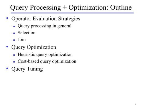
<strong>Query</strong> <strong>Processing</strong> + <strong>Optimization</strong>: Outline<br />
• Operator Evaluation Strategies<br />
• <strong>Query</strong> processing in general<br />
• Selection<br />
• Join<br />
• <strong>Query</strong> <strong>Optimization</strong><br />
• Heuristic query optimization<br />
• Cost-based query optimization<br />
• <strong>Query</strong> Tuning<br />
1
<strong>Query</strong> <strong>Processing</strong> + <strong>Optimization</strong><br />
• Operator Evaluation Strategies<br />
• Selection<br />
• Join<br />
• <strong>Query</strong> <strong>Optimization</strong><br />
• <strong>Query</strong> Tuning<br />
2
Architectural Context<br />
DDL<br />
Statements<br />
DDL<br />
Compiler<br />
DBMS<br />
DBA Staff<br />
Privileged<br />
Comm<strong>and</strong>s<br />
Casual Users<br />
Interactive<br />
<strong>Query</strong><br />
<strong>Query</strong><br />
Compiler<br />
<strong>Query</strong> Execution<br />
Plan<br />
Run-time<br />
Evaluator<br />
Transaction <strong>and</strong><br />
Data Manager<br />
Application Programmers<br />
Application<br />
Programs<br />
Precompiler<br />
DDL<br />
Statements<br />
Host Language<br />
Compiler<br />
Parametric<br />
Users<br />
Canned<br />
Transactions<br />
Data Dictionary<br />
Data Files<br />
3
Evaluation of SQL Statement<br />
• The query is evaluated in a different order.<br />
• The tables in the from clause are combined using Cartesian<br />
products.<br />
• The where predicate is then applied.<br />
• The resulting tuples are grouped according to the group by<br />
clause.<br />
• The having predicate is applied to each group, possibly<br />
eliminating some groups.<br />
• The aggregates are applied to each remaining group.<br />
The select clause is performed last.<br />
4
Overview of <strong>Query</strong> <strong>Processing</strong><br />
1. Parsing <strong>and</strong> translation<br />
2. <strong>Optimization</strong><br />
3. Evaluation<br />
4. Execution<br />
<strong>Query</strong> in high-level language<br />
Scanning, Parsing, <strong>and</strong><br />
Semantic Analysis<br />
<strong>Query</strong> <strong>Optimization</strong><br />
Intermediate form of query<br />
Execution Plan<br />
<strong>Query</strong> Code Generator<br />
Runtime Database<br />
Processor<br />
Code to execute the query<br />
Result of query<br />
5
Selection Queries<br />
• Primary key, point<br />
σ FilmID = 2 (Film)<br />
• Point<br />
σ Title = ‘Terminator’ (Film)<br />
• Range<br />
σ 1 < RentalPrice < 4 (Film)<br />
• Conjunction<br />
σ Type = ‘M’ ∧ Distributor = ‘MGM’ (Film)<br />
• Disjunction<br />
σ PubDate < 2004 ∨ Distributor = ‘MGM’ (Film)<br />
6
• Linear search<br />
Selection Strategies<br />
• Expensive, but always applicable.<br />
• Binary search<br />
• Applicable only when the file is appropriately ordered.<br />
• Hash index search<br />
• Single record retrieval; does not work for range queries.<br />
• Retrieval of multiple records.<br />
• Clustering index search<br />
• Multiple records for each index item.<br />
• Implemented with single pointer to block with first<br />
associated record.<br />
• Secondary index search<br />
• Implemented with dense pointers, each to a single record.<br />
7
Selection Strategies for Conjunctive Queries<br />
• Use any available indices for attributes involved in<br />
simple conditions.<br />
• If several are available, use the most selective index. Then<br />
check each record with respect to the remaining conditions.<br />
• Attempt to use composite indices.<br />
• This can be very efficient.<br />
• Do intersection of record pointers.<br />
• If several indices with record pointers are applicable to the<br />
selection predicate, retrieve <strong>and</strong> intersect the pointers. Then<br />
retrieve (<strong>and</strong> check) the qualifying records.<br />
• Disjunctive queries provide little opportunity for smart<br />
processing.<br />
8
Joins<br />
• Join Strategies<br />
• Nested loop join<br />
• Index-based join<br />
• Sort-merge join<br />
• Hash join<br />
• Strategies work on a per block (not per record) basis.<br />
• Need to estimate #I/Os (block retrievals)<br />
• Relation sizes <strong>and</strong> join selectivities impact join cost.<br />
• <strong>Query</strong> selectivity = #tuples in result / #c<strong>and</strong>idates<br />
<br />
‘More selective’ means smaller ‘selectivity value’<br />
• For join, #c<strong>and</strong>idates is the size of Cartesian product<br />
9
Nested Loop Join <strong>and</strong> Index-Based Join<br />
• Nested loop join<br />
• Exhaustive comparison (i.e., brute force approach)<br />
• The ordering (outer/inner) of files <strong>and</strong> allocation of buffer<br />
space is important.<br />
• Index-based join<br />
• Requires (at least) one index on a join attribute.<br />
• At times, a temporary index is created for the purpose of a<br />
join.<br />
• The ordering (outer/inner) of files is important.<br />
10
Nested Loop<br />
• Basically, for each block of the outer table (r), scan the<br />
entire inner table (s).<br />
• Requires quadratic time, O(n 2 )<br />
• Improved when buffer is used.<br />
Outer<br />
r<br />
Main Memory<br />
Buffer<br />
Scan<br />
Inner<br />
spill<br />
when full<br />
Output<br />
s<br />
11
Example of Nested-Loop Join<br />
Customer n C.CustomerID = CO.EmpId CheckedOut<br />
• Parameters<br />
r CheckedOut = 40.000 r Customer = 200<br />
b CheckedOut = 2.000 b Customer = 10<br />
n B = 6 (size of main memory buffer)<br />
• Algorithm:<br />
repeat: read (n B - 2) blocks from outer relation<br />
repeat: read 1 block from inner relation<br />
compare tuples<br />
• Cost: b outer + ( ⎡b outer / (n B -2)⎤ ) × b inner<br />
• CheckedOut as outer: 2.000 + ⎡2.000/4⎤×10 = 7.000<br />
• Customer as outer: 10 + ⎡10/4⎤×2.000 = 6.010<br />
12
Index-based Join<br />
• Requires (at least) one index on a join attribute<br />
• A temporary index can be created<br />
Scan<br />
Outer<br />
for each<br />
record of<br />
s, query<br />
in index<br />
index on r<br />
r<br />
s<br />
if joins<br />
Output<br />
spill<br />
when full<br />
Main Memory<br />
13
Example of Index-Based Join<br />
Customer n C.CustomerID = CO.EmpId CheckedOut<br />
• Cost: b outer + r outer × cost use of index<br />
• Assume that the video store has 10 employees.<br />
• There are 10 distinct EmpIDs in CheckedOut.<br />
• Assume 1-level index on CustomerID of Customer.<br />
• Iterate through all 40.000 tuples in CheckedOut (outer<br />
rel.)<br />
• 2.000 disk reads (b CheckedOut ) to scan CheckedOut<br />
• For each CheckedOut tuple, search for matching Customer<br />
tuples using index.<br />
<br />
0 disk reads for index (in main memory) + 1 disk read for actual data<br />
block<br />
• Cost: 2.000 + 40.000 × (0 + 1) = 42.000<br />
14
Sort-Merge Join<br />
• Sort each relation using multiway merge-sort<br />
• Perform merge-join<br />
Scan<br />
unsorted<br />
r<br />
r 1<br />
r 2<br />
•••<br />
sorted<br />
r<br />
Scan<br />
sorted<br />
r<br />
Main Memory<br />
•••<br />
•••<br />
•••<br />
•••<br />
Match<br />
r n<br />
sorted<br />
s<br />
Output<br />
15
External or Disk-based Sorting<br />
• Relation on disk often too large to fit into memory<br />
• Sort in pieces, called runs<br />
Scan<br />
r<br />
Main Memory<br />
Buffer (N blocks)<br />
Output<br />
when sorted<br />
r 1<br />
r 2<br />
•••<br />
r M div N<br />
Unsorted relation<br />
(M blocks)<br />
r last<br />
Runs<br />
(M div N runs each of<br />
size N blocks, <strong>and</strong> maybe one<br />
last run of < N leftover blocks)<br />
16
External or Disk-based Sorting, Cont.<br />
• Runs are now repeatedly merged<br />
• One memory buffer used to collect output<br />
r 1<br />
r 2<br />
•••<br />
Main Memory<br />
Buffer (N blocks)<br />
Output<br />
when merged<br />
m 1<br />
m 2<br />
•••<br />
Main Memory<br />
Buffer (N blocks)<br />
r N -1<br />
m last - 1<br />
•••<br />
r M div N<br />
output<br />
m last<br />
output<br />
r last<br />
sorted runs<br />
(N blocks each)<br />
Merged runs<br />
((M div N) div N-1) runs each of<br />
size N*N-1 blocks, <strong>and</strong> maybe one<br />
last run of < N*N-1 leftover blocks)<br />
17
External Sorting (Multiway Merge Sort)<br />
• Buffer size is n B = 4 (N)<br />
Orginal rel.<br />
32 5 1712 1 14 8 3 3130232629 2 2511 6 7 151628 4 9 221821102013272419<br />
Initial runs<br />
First merge<br />
Second merge<br />
5 121732 1 3 8 14 23263031 2 112529 6 7 1516 4 9 2228 10182021 13192427<br />
1 3 5 8 1214172326303132 2 4 6 7 9 11151622252829 1013181920202427<br />
1 2 3 4 5 6 7 8 9 1011121314151617181920212223242526272829303132<br />
• Cost: 2 × b relation + 2 × b relation ×⎡log nB -1 (b relation /n B )⎤<br />
• 2 × 32 + 2 × 32 × log 3 (32/4) = 192<br />
18
Example of Sort-Merge Join<br />
• Cost to sort CheckedOut (b CheckedOut = 10)<br />
• Cost Sort ChecedOut = 2 × 2.000 + 2 × 2.000 × ⎡log 5 (2.000/6)⎤ = 20.000<br />
• Cost to sort Customer relation (b Customer = 10)<br />
• Cost Sort Customer = 2 × 10 + 2 × 10 × ⎡log 5 (10/6)⎤ = 40<br />
• Cost for merge join<br />
• Cost to scan sorted Customer + cost to scan sorted CheckedOut<br />
• Cost merge join = 10 + 2.000 = 2.010<br />
• Cost sort-merge join = Cost Sort Customer + Cost Sort ChecedOut + Cost merge join<br />
• Cost sort-merge join = 20.000 + 40 + 2.010 = 22.050<br />
19
Hash Join<br />
• Hash each relation on the join attributes<br />
• Join corresponding buckets from each relation<br />
Buckets from r<br />
Buckets from s<br />
r 1<br />
r 1<br />
n<br />
s 1<br />
r 1 n s 1<br />
Relation<br />
r<br />
r 2<br />
•••<br />
r 2<br />
•••<br />
n<br />
s 2<br />
•••<br />
r 2 n s 2<br />
r n<br />
r n<br />
n<br />
s n<br />
r n n s n<br />
Hash r (same for s)<br />
Join corresponding r <strong>and</strong> s buckets<br />
20
Partitioning Phase<br />
• Partitioning phase: r divided into n h partitions. The<br />
number of buffer blocks is n B . One block used for<br />
reading r. (n h = n B -1)<br />
• Similar with relation s<br />
• I/O cost: 2 × (b r + b s )<br />
OUTPUT<br />
1<br />
Partitions<br />
Relation<br />
r or s<br />
. . .<br />
INPUT<br />
hash<br />
function<br />
h<br />
2<br />
n B<br />
-1<br />
1<br />
2<br />
n B<br />
-1<br />
Disk<br />
n B<br />
main memory buffers<br />
Disk<br />
21
Joining Phase<br />
• Joining (or probing) phase: n h iterations where r i n s i .<br />
Partitions<br />
of r & s<br />
• Load r i into memory <strong>and</strong> build an in-memory hash index on it using the<br />
join attribute. (h 2 needed, r i called build input)<br />
• Load s i , for each tuple in it, join it with r i using h 2 . (s i called probe input)<br />
• I/O cost: b r + b s + 4 × n h (each partition may have a partially filled block)<br />
<br />
One write <strong>and</strong> one read for each partially filled block<br />
In-memory hash table for<br />
Hash partition r i (< n B -1 blocks)<br />
func.<br />
h 2<br />
h 2<br />
Join Result<br />
Input buffer<br />
for s i<br />
Output<br />
buffer<br />
Disk<br />
n B main memory buffers<br />
Disk<br />
22
Hash Join Cost<br />
• Cost Total = Cost Partitioning + Cost Joining<br />
= 3 × (b r + b s ) + 2 × n h<br />
• Cost = 3 × (2000 + 10) + 2 × 5 = 6040<br />
• Any problem not considered?<br />
• What if n h > n B -1? I.e., more partitions than available buffer blocks!<br />
• How to solve it?<br />
OUTPUT<br />
1<br />
Relation<br />
r or s<br />
INPUT<br />
hash<br />
function<br />
. . .<br />
n B<br />
h<br />
2<br />
n B -1<br />
Disk<br />
n B main memory buffers<br />
23
Recursive Partitioning<br />
• Required if number of partitions n h is greater than<br />
number of available buffer blocks n B -1.<br />
• instead of partitioning n h ways, use n B – 1 partitions for s<br />
• Further partition the n B – 1 partitions using a different hash<br />
function<br />
• Use same partitioning method on r<br />
• Rarely required: e.g., recursive partitioning not needed for<br />
relations of 1GB or less with memory size of 2MB, with<br />
block size of 4KB.<br />
• Cost hjrp = 2 × (b r + b s ) ×⎡log nB -1 (b s ) -1⎤ + b r + b s<br />
• Cost hjrp = 2 × (2000 + 10) ×⎡log 5 (10) -1⎤ + 2000 + 10<br />
= 6030<br />
24
Cost <strong>and</strong> Applicability of Join Strategies<br />
• Nested-loop join<br />
• Brute-force<br />
• Can h<strong>and</strong>le all types of joins (=, )<br />
• Index-based join<br />
• Requires minimum one index on join attributes<br />
• Sort-merge join<br />
• Requires that the files are sorted on the join attributes.<br />
• Sorting can be done for the purpose of the join.<br />
• A variation is also applicable when secondary indices are<br />
available instead.<br />
• Hash join<br />
• Requires good hashing functions to be available.<br />
• Performance best if smallest relation fits in memory. ?<br />
25
<strong>Query</strong> <strong>Processing</strong> + <strong>Optimization</strong><br />
• Operator Evaluation Strategies<br />
• <strong>Query</strong> <strong>Optimization</strong><br />
• Heuristic <strong>Query</strong> <strong>Optimization</strong><br />
• Cost-based <strong>Query</strong> <strong>Optimization</strong><br />
• <strong>Query</strong> Tuning<br />
26
<strong>Query</strong> <strong>Optimization</strong><br />
• Aim: Transform query into faster, equivalent query<br />
equivalent query 1<br />
query<br />
equivalent query 2<br />
...<br />
equivalent query n<br />
faster<br />
query<br />
• Heuristic (logical) optimization<br />
• <strong>Query</strong> tree (relational algebra) optimization<br />
• <strong>Query</strong> graph optimization<br />
• Cost-based (physical) optimization<br />
27
<strong>Query</strong> Tree <strong>Optimization</strong> Example<br />
• What are the names of customers living on Elm Street<br />
who have checked out “Terminator”?<br />
• SQL query:<br />
SELECT Name<br />
FROM Customer CU, CheckedOut CH, Film F<br />
WHERE Title = ’Terminator’ AND F.FilmId = CH.FilmID<br />
AND CU.CustomerID = CH.CustomerID AND CU.Street = ‘Elm’<br />
• Canonical query tree<br />
π Name<br />
σ Title = ‘Terminator’ ∧ F.FilmId = CH.FilmID ∧ CU.CustomerID = CH.CustomerID ∧ CU.Street = ‘Elm’<br />
×<br />
CU<br />
×<br />
CH<br />
F<br />
Note the use of<br />
Cartesian product!<br />
28
Apply Selections Early<br />
π Name<br />
σ F.FilmId = CH.FilmID<br />
×<br />
σ CU.CustomerID = CH.CustomerID<br />
σ Title = ‘Terminator’<br />
×<br />
F<br />
σ Street = ‘Elm’<br />
CH<br />
CU<br />
29
Apply More Restrictive Selections Early<br />
π Name<br />
σ CU.CustomerID = CH.CustomerID<br />
×<br />
σ F.FilmId = CH.FilmID<br />
σ Street = ‘Elm’<br />
×<br />
CU<br />
σ Title = ‘Terminator’<br />
CH<br />
F<br />
30
Form Joins<br />
π Name<br />
n CU.CustomerID = CH.CustomerID<br />
n F.FilmId = CH.FilmID<br />
σ Street = ‘Elm’<br />
σ Title = ‘Terminator’<br />
CH<br />
CU<br />
F<br />
31
Apply Projections Early<br />
π Name<br />
n CU.CustomerID = CH.CustomerID<br />
n F.FilmId = CH.FilmID<br />
σ Street = ‘Elm’<br />
π FilmID π FilmID, CustomerID<br />
π Name, CustomerID<br />
σ Title = ‘Terminator’<br />
F<br />
CH<br />
CU<br />
32
Some Transformation Rules<br />
• Cascade of σ: σ c1 ∧ c 2 ∧ ... ∧ c n<br />
(R) = σ c1 (σ c2 (...(σ cn (R))...))<br />
• Commutativity of σ: σ c1 (σ c2 (R)) = σ c2 (σ c1 (R))<br />
• Commuting σ with π: π L (σ c (R)) = σ c (π L (R))<br />
• Only if c involves solely attributes in L.<br />
• Commuting σ with n : σ c (R<br />
n S) = σ c (R)<br />
n S<br />
• Only if c involves solely attributes in R.<br />
• Commuting σ with set operations: σ c (R θ S) = σ c (R) θ σ c (S)<br />
• Where θ is one of ∪, ∩, or -.<br />
• Commutativity of ∪, ∩, <strong>and</strong> n: R θ S = S θ R<br />
• Where θ is one of ∪, ∩ <strong>and</strong> n.<br />
• Associativity of n, ∪, ∩: (R θ S) θ T = R θ (S θ T)<br />
33
Transformation Algorithm Outline<br />
• Transform a query represented in relational algebra to<br />
an equivalent one (generates the same result.)<br />
• Step 1: Decompose σ operations.<br />
• Step 2: Move σ as far down the query tree as possible.<br />
• Step 3: Rearrange leaf nodes to apply the most<br />
restrictive σ operations first.<br />
• Step 4: Form joins from × <strong>and</strong> subsequent σ operations.<br />
• Step 5: Decompose π <strong>and</strong> move down the query tree as<br />
far as possible.<br />
• Step 6: Identify c<strong>and</strong>idates for combined operations.<br />
34
Heuristic <strong>Query</strong> <strong>Optimization</strong> Summary<br />
• Heuristic optimization transforms the query-tree by<br />
using a set of rules (Heuristics) that typically (but not<br />
in all cases) improve execution performance.<br />
• Perform selection early (reduces the number of tuples)<br />
• Perform projection early (reduces the number of attributes)<br />
• Perform most restrictive selection <strong>and</strong> join operations (i.e.<br />
with smallest result size) before other similar operations.<br />
• Generate initial query tree from SQL statement.<br />
• Transform query tree into more efficient query tree, via<br />
a series of tree modifications, each of which hopefully<br />
reduces the execution time.<br />
• A single query tree is involved.<br />
35
Cost-Based <strong>Optimization</strong><br />
• Use transformations to generate multiple c<strong>and</strong>idate<br />
query trees from the canonical query tree.<br />
• Statistics on the inputs to each operator are needed.<br />
• Statistics on leaf relations are stored in the system catalog.<br />
• Statistics on intermediate relations must be estimated; most<br />
important is the relations' cardinalities.<br />
• Cost formulas estimate the cost of executing each<br />
operation in each c<strong>and</strong>idate query tree.<br />
• Parameterized by statistics of the input relations.<br />
• Also dependent on the specific algorithm used by the operator.<br />
• Cost can be CPU time, I/O time, communication time, main<br />
memory usage, or a combination.<br />
• The c<strong>and</strong>idate query tree with the least total cost is<br />
selected for execution.<br />
36
• Per relation<br />
• Tuple size<br />
Relevant Statistics<br />
• Number of tuples (records): r<br />
• Load factor (fill factor), percentage of space used in each<br />
block<br />
• Blocking factor (number of records per block): bfr<br />
• Relation size in blocks: b<br />
• Relation organization<br />
• Number of overflow blocks<br />
37
• Per attribute<br />
Relevant Statistics, cont.<br />
• Attribute size <strong>and</strong> type<br />
• Number of distinct values for attribute A: d A<br />
• Probability distribution over the values<br />
• Representation, e.g., compressed<br />
• Selection cardinality specifies the average size of<br />
σ A = a (R) for an arbitrary value a. (s A )<br />
<br />
Could be maintained for the “average” attribute value, or on a pervalue<br />
basis, as a histogram.<br />
38
• Per Index<br />
• Base relation<br />
Relevant Statistics, cont.<br />
• Indexed attribute(s)<br />
• Organization, e.g., B + -Tree, Hash, ISAM<br />
• Clustering index?<br />
• On key attribute(s)?<br />
• Sparse or dense?<br />
• Number of levels (if appropriate)<br />
• Number of first-level index blocks: b 1<br />
• General<br />
• Available main memory blocks: N<br />
39
Cost Estimation Example<br />
4<br />
π Name<br />
⋈ CU.CustomerID = R.CustomerID<br />
⋈ F.FilmId = R.FilmID<br />
2 3<br />
π FilmID, CustomerID, Name<br />
π FilmID π FilmID, CustomerID<br />
σ<br />
1<br />
Street = ‘Elm’<br />
σ Title = ‘Terminator’<br />
F<br />
R<br />
CU<br />
40
• Statistics<br />
Operation 1: σ followed by a π<br />
• Relation statistics: r Film = 5,000 b Film = 50<br />
• Attribute statistics: s Title = 1<br />
• Index statistics: Secondary Hash Index on Title.<br />
• Result relation size: 1 tuple.<br />
• Operation: Use index with ‘Terminator’, then project<br />
on FilmID. Leave result in main memory (1 block).<br />
• Cost (in disk accesses): C 1 = 1 +1 = 2<br />
41
• Statistics<br />
Operation 2: n followed by a π<br />
• Relation statistics: r CheckedOut = 40,000 b CheckedOut = 2,000<br />
• Attribute statistics: s FilmID = 8<br />
• Index statistics: Secondary B + -Tree Index for CheckedOut on<br />
FilmID with 2 levels.<br />
• Result relation size: 8 tuples.<br />
• Operation: Index join using B + -Tree, then project on<br />
CustomerID. Leave result in main memory (one block).<br />
• Cost: C 2 = 1 +1 + 8 = 10<br />
42
• Statistics<br />
Operation 3: σ followed by a π<br />
• Relation statistics: r Customer = 200 b Customer = 10<br />
• Attribute statistics:s Street = 10<br />
• Result relation size: 10 tuples.<br />
• Operation: Linear search of Customer. Leave result in<br />
main memory (one block).<br />
• Cost: C 3 = 10<br />
43
Operation 4: n followed by a π<br />
• Operation: Main memory join on relations in main<br />
memory.<br />
• Cost: C 4 = 0<br />
• Total cost: C Ci = 2+<br />
10+<br />
10+<br />
0 = 22<br />
4<br />
=∑<br />
i= 1<br />
44
Comparison<br />
• Heuristic query optimization<br />
• Sequence of single query plans<br />
• Each plan is (presumably) more efficient than the previous.<br />
• Search is linear.<br />
• Cost-based query optimization<br />
• Many query plans generated.<br />
• The cost of each is estimated, with the most efficient chosen.<br />
• Search is multi-dimensional, usually using dynamic<br />
programming. Still can be very expensive.<br />
• Hybrid way<br />
• Systems may use heuristics to reduce the number of choices<br />
that must be made in a cost-based fashion.<br />
45
<strong>Query</strong> <strong>Processing</strong> + <strong>Optimization</strong><br />
• Operator Evaluation Strategies<br />
• <strong>Query</strong> <strong>Optimization</strong><br />
• <strong>Query</strong> Tuning<br />
46
<strong>Query</strong> Tuning<br />
• <strong>Query</strong> optimization is a very complex task.<br />
• Combinatorial explosion.<br />
• The task is to find one good query evaluation plan, not the<br />
best one.<br />
• No optimizer optimizes all queries adequately.<br />
• There is a need for query tuning.<br />
• All optimizers differ in their ability to optimize queries,<br />
making it difficult to prescribe principles.<br />
• Having to tune queries is a fact of life.<br />
• <strong>Query</strong> tuning has a localized effect <strong>and</strong> is thus relatively<br />
attractive.<br />
• It is a time-consuming <strong>and</strong> specialized task.<br />
• It makes the queries harder to underst<strong>and</strong>.<br />
• However, it is often a necessity.<br />
• This is not likely to change any time soon.<br />
47
<strong>Query</strong> Tuning Issues<br />
• Need too many disk accesses (eg. Scan for a point<br />
query)?<br />
• Need unnecessary computation?<br />
• Redundant DISTINT<br />
SELECT DISTINCT cpr#<br />
FROM Employee<br />
WHERE dept = ‘computer’<br />
• Relevant indexes are not used? (Next slide)<br />
• Unnecessary nested subqueries?<br />
• ……<br />
48
Join on Clustering Index, <strong>and</strong> Integer<br />
SELECT Employee.cpr#<br />
FROM Employee, Student<br />
WHERE Employee.name = Student.name<br />
--><br />
SELECT Employee.cpr#<br />
FROM Employee, Student<br />
WHERE Employee.cpr# = Student.cpr#<br />
49
Nested Queries<br />
• Nested block is optimized independently, with the outer tuple<br />
considered as providing a selection condition.<br />
• Outer block is optimized with the cost of ‘calling’ nested block<br />
computation taken into account.<br />
• Implicit ordering of these blocks means that some good<br />
strategies are not considered. The non-nested version of the<br />
query is typically optimized better.<br />
SELECT S.sname<br />
FROM Sailors S<br />
WHERE EXISTS<br />
(SELECT *<br />
FROM Reserves R<br />
WHERE R.bid=103<br />
AND R.sid=S.sid)<br />
Nested block to optimize:<br />
SELECT *<br />
FROM Reserves R<br />
WHERE R.bid=103<br />
AND S.sid= outer value<br />
Equivalent non-nested query:<br />
SELECT S.sname<br />
FROM Sailors S, Reserves R<br />
WHERE S.sid=R.sid<br />
AND R.bid=103<br />
50
Unnesting Nested Queries<br />
• Uncorrelated sub-queries with aggregates.<br />
• Most systems would compute the average only once.<br />
SELECT ssn<br />
FROM emp<br />
WHERE salary > (SELECT AVG(salary) FROM emp)<br />
• Uncorrelated sub-queries without aggregates.<br />
SELECT ssn<br />
FROM emp<br />
WHERE dept IN (SELECT dept FROM techdept)<br />
• Some systems may not use emp's index on dept, so a<br />
transformation is desirable.<br />
SELECT ssn<br />
FROM emp, techdept<br />
WHERE emp.dept = techdept.dept<br />
When is this<br />
acceptable?<br />
51
Unnesting Nested Queries, cont.<br />
• Watch out for duplicates! Consider a query <strong>and</strong> its<br />
rewritten counterpart.<br />
SELECT AVG(salary)<br />
FROM emp<br />
WHERE manager IN (SELECT manager FROM techdept)<br />
• Unnested version, with problems: (what’s the problem?)<br />
SELECT AVG(salary)<br />
FROM emp, techdept<br />
WHERE emp.manager = techdept.manager<br />
• This query may yield wrong results! A solution:<br />
SELECT DISTINCT (manager) INTO temp<br />
FROM techdept<br />
SELECT AVG(salary)<br />
FROM emp, temp<br />
WHERE emp. manager = temp. manager<br />
52
Summary<br />
• <strong>Query</strong> processing & optimization is the heart of a<br />
relational DBMS.<br />
• Heuristic optimization is more efficient to generate, but<br />
may not yield the optimal query evaluation plan.<br />
• Cost-based optimization relies on statistics gathered on<br />
the relations (the default in most DBMSs).<br />
• Until query optimization is perfected, query tuning will<br />
be a fact of life.<br />
53